Jintai Ding1, Ray Perlner2, Albrecht Petzoldt2, and Daniel Smith-Tone2,3 1Department of Mathematical Sciences, University of Cincinnati,
Cincinnati, Ohio, USA
2National Institute of Standards and Technology, Gaithersburg, Maryland, USA
3Department of Mathematics, University of Louisville, Louisville, Kentucky, USA
[email protected],[email protected],
[email protected],[email protected]
Abstract. The HFEv- signature scheme is one of the most studied mul-tivariate schemes and one of the major candidates for the upcoming stan-dardization of post-quantum digital signature schemes. In this paper, we propose three new attack strategies against HFEv-, each of them using the idea of projection. Especially our third attack is very effective and is, for some parameter sets, the most efficient known attack against HFEv-. Furthermore, our attack requires much less memory than direct and rank attacks. By our work, we therefore give new insights in the security of the HFEv- signature scheme and restrictions for the parameter choice of a possible future standardized HFEv- instance.
Key words: Multivariate Cryptography, HFEv-, MinRank, Gr¨obner Basis, Projection
1
Introduction
Multivariate Cryptography is one of the main candidates for establishing cryp-tosystems which resist attacks with quantum computers (so called Post-Quantum Cryptosystems). Especially in the area of digital signatures, there exists a large number of practical multivariate schemes such as UOV [13] and Rainbow [7]. Another well known multivariate signature scheme is the HFEv- signature scheme, which was first proposed by Patarin, Courtois and Goubin in [17]. Most notably about this scheme are its very short signatures, which are currently the shortest signatures of all existing schemes (both classical and post-quantum).
In this paper we propose three new attacks against the HFEv- signature scheme, each of them using the idea of projection. This means that each of our attacks reduces the number of variables in the system by guessing, either before or after the attack itself.
distinguishing attack is to remove the vinegar modifier. This allows the attacker to follow up with any key recovery or signature forgery attack applicable to an HFE- instance with the same degree bound and the same number of removed equations as the original HFEv- instance. The attack is very effective and outper-forms, for selected parameter sets, all other attacks against HFEv-. Furthermore, the memory requirements of our attack are far less than those of direct and Min-Rank attacks.
The rest of the paper is organized as follows. In Section 2, we give a short overview of multivariate cryptography and introduce the HFEv- cryptosystem, while Section 3 reviews the previous cryptanalysis of this scheme. Section 4 de-scribes our first two attacks, which combine the MinRank attack with the idea of projection. In Section 5, we present then our distinguishing attack, whose com-plexity is analyzed in Section 6. Finally, Section 7 presents an idea to improve the complexity of our attack, and Section 8 concludes the paper.
2
Hidden Field Equations
2.1 Multivariate cryptography
The basic objects of multivariate cryptography are systems of multivariate quadratic polynomials over a finite field F. The security of multivariate schemes is based on theMQ Problem of solving such a system. The MQ Problem is proven to be NP-Hard even for quadratic polynomials over the field GF(2) [12] and believed to be hard on average (both for classical and quantum computers).
To build a multivariate public key cryptosystem (MPKC), one starts with an easily invertible quadratic map F :Fn →
Fm(central map). To hide the
struc-ture ofF in the public key, we compose it with two invertible affine (or linear) mapsT :Fm→Fm andU :Fn→Fn. Thepublic key of the scheme is therefore
given by P =T ◦ F ◦ U :Fn →Fm. The relation between the easily invertible
central mapFand the public keyPis referred to as a morphism of polynomials. Definition 1 Two systems of multivariate polynomials F andG are said to be related by a morphismiff there exist two affine mapsT,U such thatG=T ◦F ◦U.
Theprivate key consists of the three mapsT,F andU and therefore allows to invert the public key.
To generate a signature for a document (hash value) h ∈ Fm, one computes
recursively x=T−1(h)∈
Fm,y=F−1(x)∈Fn andz=U−1(y)∈Fn.
To check the authenticity of a signature z ∈ Fn, one simply computes h0 =
P(z)∈ Fm. If the result is equal to h, the signature is accepted, otherwise
re-jected.
Signature Generation
Signature Verification
h∈Fm - x∈Fm - y∈Fn - z∈Fn
6
P
T−1 F−1 U−1
Fig. 1.Signature Generation and Verification for Multivariate Signature Schemes
2.2 HFE Variants
The HFE encryption scheme was proposed by J. Patarin in [16]. The scheme belongs to the BigField family of multivariate schemes, which means that it uses a degree n extension field E of F as well as an isomorphism φ :Fn → E. The
central map is a univariate polynomial map overEof the form
F(X) =
qi+qj≤D X
0≤i,j
αijXq
i+qj
+ qi≤D
X
i=0 βiXq
i
+γ.
Due to the special structure ofF, the map ¯F =φ−1◦ F ◦φis a quadratic map over the vector space Fn. In order to hide the structure of F in the public key,
¯
F is composed with two affine mapsT andU, i.e.P =T ◦F ◦ U.¯
After the basic scheme was broken by direct [11] and rank attacks [14], sev-eral versions of HFE for digital signatures have been proposed. Basically, these schemes use two different techniques: the minus and the vinegar modification. For the HFEv- signature scheme [17], the central mapF has the form
F(X, xV) =
qi+qj≤D X
0≤i,j
αijXq
i+qj
+ qi≤D
X
i=0
βi(x1, . . . , xv)Xqi+γ(x1, . . . , xv),
where βi and γ are linear and quadratic maps in the vinegar variables xV = (x1, . . . , xv) respectively. Definingψ:Fn+v→E×Fvbyψ=φ×idv, the public
key has the form
P=T ◦φ−1◦ F ◦ψ◦ U :Fn+v→Fn−a
with two affine mapsT :Fn →Fn−aandU :Fn+v→Fn+v, and is a multivariate
quadratic map with coefficients and variables overF.
Signature Generation: To generate a signature z for a document d, one uses a hash function H:{0,1}? →
Fn−a to compute a hash valueh=H(d)∈Fn−a
and performs the following four steps
2. Choose random values for the vinegar variables x1, . . . , xv and substitute them into the central map to obtain the parametrized mapFV.
3. Solve the equation FV(Y) = X over the extension field E by Berlekamp’s algorithm.
4. Computey=φ−1(Y) and the signaturez∈Fn+vbyz=U−1(y||x1||. . .||xv).
Signature Verification: To check the authenticity of a signature z∈ Fn+v, the verifier computes h = H(d) and h0 = P(z). If h0 = h holds, the signature is accepted, otherwise rejected.
3
Previous Cryptanalysis
3.1 Direct Algebraic Attack
The direct algebraic attack is the most straightforward way to attack a multi-variate cryptosystem such as HFE(v-). In this attack, one considers the public equation P(z) = has an instance of the MQ-Problem. In the case of HFEv-, the public system is slightly underdetermined. In order to make the solution space zero dimensional, one therefore fixes some of the variables in order to get a determined system before applying an algorithm like XL [4] or a Gr¨obner basis method such asF4 or F5 [9, 10]. In some cases one gets better results by guess-ing additional variables, even if this requires to run the Gr¨obner basis algorithm several times (hybrid approach [1]).
Experiments have shown that the public systems of HFE and its variants can be solved significantly faster than random system [11, 15]. This phenomenon was studied by Ding et al. in a series of papers [5, 6, 8]. In [8] it was shown that the degree of regularity of solving an HFEv- system is upper bounded by
dreg,HFEv−≤
((q−1)·(r+a+v−1)
2 + 2 qeven andr+aodd (q−1)·(r+a+v)
2 + 2 otherwise
. (1)
3.2 MinRank
The historically most effective attack on the HFE family of cryptosystems is the MinRank attack which exploits the algebraic consequence of a low degree bound D. This low degree bound leads to the fact that the central map has a low Q-rank.
Definition 2 The Q-rank of a multivariate quadratic mapf :Fn→Fnover the
finite fieldFwithqelements is the rank of the quadratic formQonE[X0, . . . , Xn−1]
defined by Q(X0, . . . , Xn−1) = φ◦f ◦φ−1(X), under the identification X0 = X, X1=Xq, . . . , X
n−1=Xq
n−1
As an example, consider an odd characteristic instance of HFE. We may write the homogeneous quadratic part of F as
h
X Xq· · · Xqn−1i
α0,0 α00,1 · · · α00,d−1 0· · · 0 α00,1 α1,1 · · · α01,d−1 0· · · 0
..
. ... . .. ... ... . .. ... α0
0,d−1α01,d−1· · · αd−1,d−10· · · 0
0 0 · · · 0 0· · · 0
..
. ... . .. ... ... . .. ...
0 0 · · · 0 0· · · 0
X Xq .. . Xqn−1
,
whereα0i,j =12αi,jandd=dlogq(D)e. Clearly, this quadratic form over the ring
E[X0, . . . , Xn−1] has rank d, and thus the HFE central map has Q-rank d. The first iteration of the MinRank attack is the Kipnis-Shamir (KS) attack of [14]. Via polynomial interpolation, the public key can be expressed as a quadratic polynomial G over the degree nextension field E. By construction there is an F-linear map T−1 such that T−1◦G has rank d, thus there is a rank d
ma-trix that is an E-linear combination of the Frobenius powers of G. This turns
recovery of the transformationT into the solution of a MinRank problem overE.
A significant improvement to this method for HFE is the key recovery attack of [2]. The first significant observation made was that an E-linear combination of the public polynomials has low rank as a quadratic form over E. By con-structing a formal linear combination of the public polynomials with variable coefficients, one can collect the polynomials representing (d+ 1)×(d+ 1) minors of this linear combination, which must be zero by the Q-rank bound. The ad-vantage this technique offers is that the coefficients of the polynomial are in F; thus, the Gr¨obner basis calculation can be performed over F, while the variety is computed overE. Thisminors modeling method is significantly more efficient
than the KS-attack when the number of equations is similar to the number of variables. (In contrast, for schemes such as ZHFE, see [20], it seems that the KS modeling is more efficient, probably due to the large number of variables in the Gr¨obner basis calculation, see [3].) The complexity of the KS-attack with minors modeling is asymptotically O(n(dlogq(D)e+1)ω), where 2≤ ω ≤ 3 is the
linear algebra constant.
The MinRank approach can also be effective in attacking HFE-. The key ob-servation in [21] is that not only does the removal of an equation increase the Q-rank by merely one, there is also a basis in which it only increases the degree by a factor ofq. Thus HFE- schemes with large base fields are vulnerable to the minors modeling method of [2], even when multiple equations are removed. The complexity of the KS-attack with minors modeling for HFE- is asymptoticaly O(n(dlogq(D)e+a+1)ω), whereais the number of equations removed and 2≤ω≤3
4
Variants of MinRank with Projection
As first explicitly noted in [8], the Q-rank of the central map is increased by v with the introduction of v vinegar variables and therefore the min-Q-rank of HFEv- isdlogq(D)e+a+v. We now discuss techniques for turning this observation into a key recovery attack. From this point on, let rdenote dlogq(D)e, that is, the Q-rank of the HFE component of the central map.
4.1 MinRank then Projection
The simplest way to attempt an attack utilizing the low Q-rank of the cen-tral map of HFEv- is to directly apply a MinRank attack and then attempt to discover the vinegar subspace. To this end, consider the representation Φ :
E→ Adefined by Φ(X) = (X, Xq, . . . , Xq
n−1
). We may map directly from an n-dimensional vector space overFto Avia right multiplication by the matrix
Mn =
1 1 · · · 1
θ θq · · · θqn−1 θ2 θ2q · · · θ2qn−1
..
. ... . .. ... θn−1θ(n−1)q · · · θ(n−1)qn−1
,
with the choice of a primitive element E = F(θ). Right multiplication by Mn corresponds to the linear mapΦ◦φ.
We may incorporate the vinegar variables into the picture by simply appending them toA. Specifically, define the map Mfn :Fn+v →A×Fv by right
multipli-cation by the matrix
f
Mn=
Mn 0n×v 0v×n Iv
,
where Iv is the identity matrix. We may then represent any HFEv- map as a single (n+v)×(n+v) matrix with coefficients inE. Note specifically that any function bilinear with respect to the vinegar variablexn and the HFE variables x0, . . . , xn−1 can be encoded in row and/or columnnof the quadratic form
xQx>=xfMnRMf>nx>,
whereR∈ M(n+v)×(n+v)(E).
example the following shape forF∗0:
α0,0 · · · α0,d−1 0· · · 0 β0,n · · · β0,n+v−1 ..
. . .. ... ... . .. ... ... . .. ... α0,d−1 · · · αd−1,d−1 0· · · 0 βd−1,n · · · βd−1,n+v−1
0 · · · 0 0· · · 0 0 · · · 0
..
. . .. ... ... . .. ... ... . .. ...
0 · · · 0 0· · · 0 0 · · · 0
β0,n · · · βd−1,n 0· · · 0 βn,n · · · βn,n+v−1 ..
. . .. ... ... . .. ... ... . .. ... β0,n+v−1· · · βd−1,n+v−10· · · 0βn,n+v−1· · · βn+v−1,n+v−1
.
Here we see that rank(F∗0) = r+v. The structure of F∗1 is similar with the upper left HFE block consisting ofαi,j shifted down and to the right and raised to the power ofq, and the symmetric blocks of mixing monomials shifted down and to the right with a more complicated function applied to theβi,jcoefficients to respect the Frobenius map.
Now let U,Tand Pi be the matrix representations of the affine isomorphisms U and T and the public quadratic forms Pi, respectively. Then we derive the relation
(P1, . . . ,Pn)T−1Mn= (UfMnF∗0Mfn>U>, . . . ,UMfnF∗(n−1)Mf>nU>).
ThusUMfnF∗0fM>nU> is anE-linear combination of the public quadratic forms.
SinceUMfn is invertible, the rank of this linear combination is the rank ofF∗0, which isr+v.
Following the analysis of [21, Theorem 2], we see that the effect of the minus modifier on the matrix representation of f overA×Fv is to add to it constant
multiples of itself with a cyclic shift of the rows and columns down and to the right within the HFE block. Thus for HFEv-,F∗0has the shape given in Figure 2. The rank of this quadratic form isr+a+v.
The solution of the MinRank instance provides an equivalent transformationT0 to the output transformation (up to the choice of extension to full rank) and a matrixL representing the low Q-rank quadratic formU0fMnFb∗0fM>nU0> over
A×Fv, whereP =T0◦φ−1◦fb◦φ◦U0 for an equivalent private key (T0,f , Uˆ 0).
Now that the correct output transformation is recovered, it remains to recover the vinegar subspace ofL=U0fMnFb∗0Mf>nU0>.
First, note that the kernel K of L is orthogonal to the vinegar subspace, so we may simplify the analysis by projecting to Lb which acts on the orthogonal
complement of a codimension one subspace of the kernel. The strategy now is to compose codimension one projection mappings π with Lb to filter out the
vinegar variables. It suffices to choose projections whose kernels are orthogonal to ker(Lb).
Fig. 2.The shape of the matrix representation of the central map of HFEv- overA×Fv.
The shaded areas represent possibly nonzero entries.
empty, the rank ofΠLΠb >should remain the same. To see this, note that by an
argument symmetric to that of [21, Lemma 1] we may equivalently defineLb◦π
by
b
L◦π=U−1◦[(φ◦π1◦φ−1◦S1)×π2]◦S2,
where S1 : Fn → Fn is nonsingular, S2 : Fn+v → Fn×Fv is an isomorphism,
π1 : E →E has degree at most qn−r−a (since the intersection of the image of
b
L◦πand the HFE subspace is at least (r+a)-dimensional) and π2 :Fv →
Fv
is linear. Since the degree bound of the central HFE quadratic form isqr+a, the highest monomial degree in the composition ofπ2 with this map is bounded by qn−1, thus the polynomialsπ1, πq
1, . . . , π qr+a
1 are linearly independent.
The probability that the linear form defining ker(π) which is orthogonal to the kernel of Lb lies in the vinegar subspace is q−(r+a+1). Once such a vector is
recovered, this step is repeated on the orthogonal complement of the discovered vectors until a basis for the vinegar subspace is found. Thus the complexity of this method is
CompM P =O
n+r+v+ 1
r+a+v+ 1
ω
+ (r+a+v+ 1)ωqr+a+1
,
where 2≤ω≤3 is the linear algebra constant.
4.2 Projection then MinRank
less than r+a+v. The probability this occurs isqk−n=q−(r+a+v).
Generalizing, we may project further in an attempt to eliminate possibly more vinegar variables and reduce the rank further. As long as the image of π is of dimension at least the sum of√n−aand the target rank, the minors system is still fully determined. Therefore, consider eliminating c vinegar variables. This requireskto be at leastn−a−r+c−√n−a. The probability that there is a c-dimensional intersection between the kernel ofπ and the vinegar subspace is thenqc(k−n)−(c2)≥q(
c+1
2 )−cr−ca−c √
n−a.
Once at least one vinegar variable is found, the new basis can be utilized to filter out the remaining vinegar variables as in the previous method. The complexity of the this method is
CompP M =O
qc(r+a+ √
n−a)−(c+1 2 )
n+r+v−c+ 1
r+a+v−c+ 1
ω
.
5
The Distinguishing attack
In this section we present our distinguishing attack against the HFEv- signature scheme. We restrict to the case of F= GF(2). The idea of the attack is closely related to the direct attacks with projection (also known as the hybrid approach). We define
V = span(Un+1,Un+2, . . . ,Un+v),
where Ui denotes thei-th component of the affine transformationU : Fn+v →
Fn+v. Therefore,Vis the space spanned by the affine representations of the
vine-gar variablesx1, . . . , xv. Our attack is based on the following two observations. – Consider the two HFEv- public keys P1 = HFEv−(n, D, a, v1) and P2 =
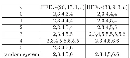
HFEv−(n, D, a, v2). Before applying a Gr¨obner basis algorithm to the sys-tems, we fix ina+v1 variables inP1 anda+v2 variables inP2 to get de-termined systems. As shown in Table 1 and Figure 3, direct attacks against these systems behave differently. In particular, we can distinguish between determined instances of the two systemsP1 and P2 by looking at the step degrees of theF4 algorithm. This remains possible, even when adding (not too many) additional linear equations to the systemsP1andP2(thus guess-ing some of the variables) before applyguess-ing a Gr¨obner basis method (hybrid approach).
– Let us consider the special case where v2 = v1−1 holds. By adding one linear equation` ∈ V to P1, we remove the influence of one of the vinegar variables form the systemP1. A direct attack against the so obtained system P0
1 therefore behaves in exactly the same way as a direct attack against the systemP2(see Table 2).
5.1 The Distinguisher
v HFEv-(26,17,1, v) HFEv-(33,9,3, v)
0 2,3,4,3,4 2,3,4,4,4
1 2,3,4,4,4 2,3,4,5,4
2 2,3,4,5,4 2,3,4,5,5
3 2,3,4,5,5 2,3,4,5,5,5,5,5,6 4 2,3,4,5,5,5,5,5 2,3,4,5,6,6
5 2,3,4,5,6
random system 2,3,4,5,6 2,3,4,5,6,6
Table 1. Step degrees of the F4 algorithm against determined HFEv- systems for different values ofv
We start with an HFEv- public keyP = HFEv−(n, D, a, v).P consists ofn−a quadratic equations in n+v variables over the field GF(2). After adding the field equations{x2
i−xi :i= 1, . . . , n+v}, we appendkrandomly chosen linear equations`1, . . . , `k to the system. Therefore, our new systemP0 consists of
– then−aquadratic HFEv- equations from P – n+v field equationsx2i −xi= 0 (i= 1, . . . , n+v) – thek linear equations`1, . . . , `k.
Altogether, the systemP0 consists of 2n−a+v+kequations inn+vvariables. After having constructed the system P0, we solve it via a Gr¨obner basis algo-rithm. Due to observation 2, the behaviour of this algorithm should depend on the fact whether one of the linear equations`i added to the system (or a linear combination of the `i) is an element of the vinegar space V. In fact, we can observe a difference in the step degrees of the algorithm (see Example 1 below). Formally written, we can use our technique to distinguish between the two cases
span(`1, . . . , `k)∩ V =∅and
span(`1, . . . , `k)∩ V 6=∅. (2) However, in most cases that span(`1, . . . , `k)∩ V 6=∅, the intersection contains only a single equation ˜`.
Remark: We have to note here that the numberkof linear equations added to the systemP is upper bounded by a value ¯k(n, D, a, v). When adding more than ¯
k linear equations to the system, a distinction between the two cases of (2) is no longer possible.
Example 1: We consider HFEv- systems with (n, D, a) = (33,9,3) and varying values ofv∈ {0, . . . ,4}. The resulting HFEv- public keys are systems ofn−a= 30 quadratic equations in n+v variables. After appending the field equations {x2
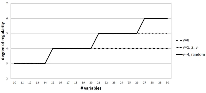
reduce the effective number of variables in our systems. Figure 3 shows the degree of regularity of a direct attack usingF4against the (projected) systems. For comparison, the figure also contains data for a random system of the same size.
Fig. 3.Direct attack against (projected) HFEv- systems with (n, D, a) = (33,9,3) and varying values ofv
As Figure 3 shows, there exists, for every parameter set (n, D, a, v) a number ¯k such that
1) When adding less than ¯klinear equations to the system, the degree of regu-larity of a direct attack against the projected system is the same as that of a direct attack against the unprojected system.
2) When adding k ≥ ¯k linear equations, the system behaves exactly like a random system of the same size.
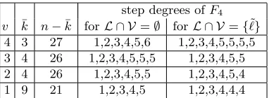
Let us now look at our distinguisher. For this, we skip the parameter set (n, D, a, v) = (33,9,3,0) since, in this case,V =∅ holds. However, as Table 2 shows, we can, for each of the values v ∈ {1, . . . ,4}, disitnguish between the two cases of (2). For abbreviation, we use in the tableL:= span(`1, . . . , `¯k). Note that the evolu-tion of the step degrees for HFEv-(33,9,3,4) is the same as for a random system of the same size.
5.2 The Attack
Based on the distinguisher presented in the previous section, we can construct an attack against HFEv- as follows.
step degrees ofF4 v ¯k n−¯k forL ∩ V =∅ forL ∩ V={`˜}
4 3 27 1,2,3,4,5,6 1,2,3,4,5,5,5,5 3 4 26 1,2,3,4,5,5,5 1,2,3,4,5,5 2 4 26 1,2,3,4,5,5 1,2,3,4,5,4 1 9 21 1,2,3,4,5 1,2,3,4,4,4
Table 2.Distinguisher Experiments on HFEv-(33,9,3, v) systems for different values ofv
`1, . . . , `k such that span(`1, . . . , `k)∩ V ={`1˜}. Using this, we can determine the exact form of ˜`1 as follows. Note that there exist coefficients αi ∈ {0,1} (i= 1, . . . k) such that
˜ `1=
k
X
i=1 αi·`i.
In order to determine the exact form of this linear combination, we remove one of the linear equations (say`1) from the systemP0 and add another randomly chosen linear equation. If we still can observe a difference in the behaviour of a direct attack compared to a random choice of linear equations, we know that the coefficient α1 must be 0. Otherwise, the coefficient α1 must be 1, and we have to add`1 back to the system.
We repeat this step fori= 2, . . . , kto determine the values of all the coefficients αi (i= 1, . . . , k). This will give us the exact form of the linear equation ˜`1∈ V. We denote this technique as “remove-and-add” strategy.
Having found ˜`1, we add it to the original HFEv-(n, D, a, v) system. The re-sulting system will behave exactly like an HFEv-(n, D, a, v−1) system, and we can again use our distinguisher and repeat the above procedure to find a second linear equation ˜`2 ∈ V. Note that this will be much easier than finding ˜`1 (see next section).
After having found v linear independent equations ˜`1, . . .`˜v ∈ V and adding them to the HFEv- system, the resulting system will behave exactly like an HFE-(n,D,a) system (i.e. we have no vinegar variables any more). We can then use any attack against HFE- (e.g. [21] or a direct attack) to break the scheme. We analyze the complexity of our distinguisher and our attack in the next section. Let us shortly return to Example 1. When we start with the systemP =HFEv-(33,9,3,4), we can use our distinguisher to find a set{`1, . . . , `k} of linear equa-tions such that span(`1, . . . , `k)∩ V = {`˜1}. After having recovered the exact form of ˜`, we can append it to the systemP, which will then behave exactly like an HFEv-(33,9,3,3) system. Let us denote this new system byP(1). We can then use the distinguisher onP0 to obtain a second linear equation ˜`
an HFEv- (33,9,3,0) system. We can then break this scheme by using any attack on HFE-.
Algorithm 1Our Distinguishing Attack
Input: HFEv-(n, D, a, v) public keyP
Output: equivalent HFE-(n, D, a) public key ˜P
1: Append ¯krandomly chosen linear equations`1, . . . , `¯kin the variablesx1, . . . , xn+v
(as well as the field equationsx2i−xi= 0) to the systemP.
2: Solve the resulting quadratic system byF4. If the step degrees of theF4algorithm differ from the standard case, we know that span(`1, . . . , `k)∩ V 6=∅. Denote the
only element of this intersection by ˜`.
3: Repeat step 1 and 2 until having found a set of linear equations `1, . . . , `k such
that span(`1, . . . , `k)∩ V 6=∅
4: Determine the exact form of ˜`by sequentially removing linear equations (trial and error).
5: Append the linear equation ˜`to the systemP. The resulting systemP0
will behave exactly like an HFEv-(n,D,a,v-1) public key.
6: Repeat the above steps until having found v linear independent equations ˜
`1, . . . ,`˜k∈ V.
7: returnP˜= (P,`1, . . . ,˜ `˜v)
6
Complexity Analysis
In this section we analyze the complexity of our distinguishing attack against HFEv-.
In the first step of our attack, we have to find one linear equation ˜` ∈ V by using our distinguisher and a following application of the “remove-and-add” strategy described in the previous section. Therefore, the complexity of this first step of our attack is determined by three factors:
1. The number of times we have to run the distinguisher in order to find a set of linear equations`1, . . . , `k such that span(`1, . . . , `k)∩ V ={`˜},
2. The cost of one run of the distinguisher and 3. The cost of recovering the exact form of ˜`.
The first number is determined by
– The probability that a randomly chosen linear equation inn+vvariables is contained in the spaceV spanned by the linear representation of the vine-gar variablesUn+1, . . . ,Un+v A randomly chosen linear equation ¯`in n+v variables can be seen as a linear combination of the components ofU, i.e.
¯ `=
n+v
X
i=1
The reason for this is thatU is an invertible map fromFn+v to itself, which means that the components ofU form a basis of this space. There are 2n+v choices for the parametersλi (i = 1, . . . , n+v). On the other hand, every element ˜`of the spaceVspanned by the linear transformations of the vinegar variablesv1, . . . , vv can be written in the form
˜ `=
n+v
X
i=n+1 λi· Ui.
The probability that a randomly chosen linear ¯`equation lies inVis therefore given by
prob(¯`∈ V) = 2−n. (4)
The reason for this is that all the coefficientsλi (i= 1, . . . , n) in the repre-sentation (3) of ¯`must be zero.
– The number of linear equations (and linear combinations thereof) added to the public key. When addingklinear equations`1, . . . , `k to the public key, we do not have to consider only thekequations`1, . . . , `k itself, but also all linear combinations of the form
`= k
X
i=1 λi·`i.
The total number of linear equations we have to consider is therefore notk, but 2k.
Therefore, when addingklinear equations`1, . . . , `kto the public key, the prob-ability of finding one linear equation ˜`∈ V, is given by
prob = 1−(1−2−n)2k≈2k−n.
In order to find one linear equation ˜`∈ V, we therefore have to run our distin-guisher about 2n−k times.
A single run of our distinguisher corresponds to one run of the F4 algorithm. The cost of this can be estimated as
Complexity(F4) = 3·
n0 dreg
2
·
n0 2
,
where n0 is the number of variables in the quadratic system and d
reg is the so called degree of regularity.
25 equations, 25 variables 25 quadr. + 10 lin. equations, 35 variables step degree matrix size time degree matrix size time
1 10×36 0.0
1 20×36 0.0
1 2 25×326 0.0 2 330×631 0.0
2 3 652×2626 0.02 3 650×2626 0.02
3 4 7,894×14,498 1.27 4 7864×15568 1.34
4 5 52,488×52,956 79.86 5 52197×52665 80.26 5 6 248,705×245,506 179.34 6 248,273×108,524 182.24
Table 3.Experiments with random systems
polynomials in 25 variables, the polynomials of system B contain 35 variables. On the other hand, the system B additionally contains 10 linear equations.
As the table shows, both systems behave very similarly. Starting at step 2 (de-gree 3), there is no significant difference between the matrix sizes or the running times of the single steps between the two systems.
We can therefore conclude that the quadratic systems we consider in our distin-guishing attack (n−aquadratic equations +klinear equations inn+vvariables) behave just like systems ofn−aquadratic equations inn+v−kvariables. Compared to finding linear equations`1, . . . , `k such that span(`1, . . . , `k)∩ V= {`˜}, the cost of recovering the exact form of ˜` is negligible. Remember that ˜` can be written as a linear combination of `1, . . . , `k, i.e. ˜` = Pk
i=1λi·`i. As described in the previous section, we remove for this one linear equation`i from the systemP0. By adding a randomly chosen linear equation, we obtain a sys-tem P00 of the same dimensions. We apply the F4 algorithm against the two systems P0 and P00. If we observe a difference in the behaviorof the algorithm, we know that the coefficient λi in the above linear combination is 1. Otherwise we have λi = 0. By running this test for all i ∈ {1, . . . , k}, we can determine all the coefficients λi and therefore recover ˜`. In order to recover ˜`, we there-fore need 2·kruns of theF4algorithm, which is far less than the 2n−k F4-runs above. Therefore, we do not have to consider this step in our complexity analysis. Altogether, we can estimate the complexity of this first step of our attack by
ComplexityDistinguisher; classical= 2n−k·3·
n+v−k
dreg
2
·
n+v−k
2
. (5) In the presence of quantum computers, we can speed up the searching step of this attack using Grover’s algorithm. Such we get
ComplexityDistinguisher; quantum= 2(n−k)/2·3·
n+v−k
dreg
2
·
n+v−k
2
.
the previous section, our distinguisher fails when k is too large. We denote the maximal value ofkfor which our distinguisher works by ¯k(n, D, a, v).
In order to remove all the vinegar variables from the system P, we have to repeat the above processvtimes. However, with decreasingvwe find (see Table 2)
1) the number ¯k of linear equtions that we can add to the public system in-creases, reducing the number ofF4-runs.
2) the degree of regularity of the systems generated by our distinguisher de-creases, reducing the complexity of a singleF4-run.
Therefore, the following steps of our attack will be much faster than the first step. This means, that we can estimated the complexity of the whole attack as in formula (5).
However, in order to estimate the complexity of our attack against an HFEv-(n, D, a, v) scheme in practice, we still have to answer the following two questions. – What is the maximal number ¯kof linear equations we can add to the public
key such that our distinguisher works?
– What is the degree of regularty of the systems generated by our distin-guisher?
In order to answer these questions, we once more consider Example 1 (see pre-vious section).
First, let us consider the second question. As a comparison of Table 2 and Fig-ure 3 shows, the degree of regularity of solving the systems generated by our distinguisher corresponds exactly to the degree of regularity of an unprojected HFEv- system with parameters (n, D, a, v). As stated in [18], we can estimate this value as
dreg=br+a+v+ 7
3 c, (6)
wherer=blogq(D−1)c+ 1.
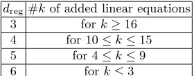
To answer the second question, let us take a closer look on the behavior of the hybrid approach against random systems (see Figure 3). We start with a random system of 30 quadratic equations in 30 variables over GF(2). After ap-pending the field equations x2
i −xi = 0 (i= 1, . . . ,30), we addk ∈ {0, . . . ,20} linear equations to the system. Table 4 shows, for which values of k we reach given values of regularity. Let us define ˆk(d) to be the maximal number of linear equations we can add to the random system, such that the degree of regularity of a direct attack against the system is greater or equal tod, i.e ˆk(6) = 3, ˆk(5) = 9 and ˆk(4) = 15.
By comparing these numbers with the values of ¯klisted in Table 2, we find ˆ
dreg#kof added linear equations
3 fork≥16
4 for 10≤k≤15 5 for 4≤k≤9
6 fork≤3
Table 4.Degree of regularity of projected random systems with 30 equations
whered?is the degree of regularity of a direct attack against an HFEv-(n, D, a, v) scheme (see equation (4)).
In order to estimate the complexity of our attack against an HFEv-(n, D, a, v) scheme, we therefore proceed as follows.
1. We compute the degree of regularity of the unprojected HFEv-(n, D, a, v) system (see equation (4)). Denote the result byd?.
2. We estimate the maximal number ¯k of linear equations we can add to the public HFEv- system by ˆk(d?). This value can be obtained as follows. The degree of regularity of a random system ofm=n−aquadratic equations inn0variables over GF(2) can be estimated as the smallest indexdfor which the coefficient ofXd in
1 1−X ·
1−X2 1−X
n0
·
1−X2 1−X4
m
is non-positive [22].
We can use this equation to determine the values of ˆk(d?).
By substituting the so obtained values of ¯kandd? into formula (5), we therefore get a close estimation of the complexity of our distinguishing attack against an HFEv-(n, D, a, v) system.
Example 2: Consider an HFEv- system over GF(2) with (n, D, a, v) = (91,5,3,2). We obtainr=blog2(D−1)c+ 1 = 3. The degree of regularity of a direct attack against the HFEv- system (with field equations) is given by
dreg=b
3 + 3 + 2 + 7 3 c= 5. Therefore, we get
Complexitydirect= 3·
88
5
2
·
88
2
≈263.9.
was chosen from the vinegar spaceV, we obtain 1; 1,2,3,3. Therefore, we can estimate the complexity of our distinguisher by
ComplexityDistinguisher= 223·
25
4
2
·
25
2
≈260.1,
which is nearly 16 times faster than a direct attack.
The complexity of a MinRank attack (MinorsModeling) against the scheme can be estimated by
ComplexityMinRank =
n+r+a+v r+a+v
2.3
≈285.2,
the complexity of classical brute force attacks by 296.1. Therefore, for the above parameter set, our attack is the most efficient classical attack against HFEv-. With regard to the memory consumption, we get
Memorydirect=
88
5
2
≈250.4,
MemoryMinRank=
n+r+a+v
r+a+v
2
≈274.3,
Memorydistinguisher=
25
4
2
≈227.3.
As these data show, our attack requires much less memory than the direct and the MinRank attack. Since attacks against large instances of multivariate schemes often fail due to memory restrictions, the small memory consumption is a huge benefit of our attack.
7
Improvements to the Direct Attack
It is possible that the average cost of the distinguishing step can be reduced by selecting the projection in a slightly nonrandom fashion. In particular, we may consider simultaneously testing a set of corankkprojectionsπwhose kernels are contained within the kernel of a single corankk+1 projection,π1. In such a case, we can treat the image of π1 in the plaintext space as being generated by the variables x1, ..., xn+v−k−1, and the image of π as being generated by the same variables plus one additional variablexn+v−k, which defines a 1-dimensional sub-space of the kernel ofπ1, which will vary depending on the choice ofπ.
Our strategy will be to first solve for allpi over the variablesx1, ..., xn+v−k−1, such that
X
pifi(π) =q(mod xn+v−k). As the above equation is equivalent to P
pifi(π1) = q, this computation can be reused for multiple different choices of π. Note also, that any solution to
P
pifi(π) =qis also a solution toPpifi(π) =q(mod xn+v−k), despite of the fact that p may contain monomials involving xn+v−k that would be removed by modular reduction. We can therefore generate solutions toP
pifi =q from linear combinations of:
1. polynomials of the formP
pifi(π) , wherepiis a solution over the variables x1, ..., xn+v−k−1 ofPpifi(π) =q(modxn+v−k); and,
2. polynomials of the formP
xn+v−kp0ifi(π), wherep0ihas degree at mostd−3. As both types of polynomial are divisible by xn+v−k in their degree-d terms, finding a linear combination of these polynomials with degreed−1 only requires finding cancellations among as many distinct monomials as would be required when solving a system with degree of regularityd−1.
It should be noted that a projection of degree k+ 1 is approximately q times more likely to have a nontrivial intersection between its kernel and the vinegar subspace as is a projection of degreek, and conditional on ker(π1) having such a nontrivial intersection, the probability that ker(π) also having a nontrivial intersection is approximately 1 inq. It is therefore optimal to chooseqdifferent π’s for eachπ1. It should further be noted that the above strategy can be applied recursively with sets ofq π1s having theirk+ 1 dimensional kernels contained within the kernel of a corankk+ 2 projectionπ2. While it is clear that a large saving is possible when projections that eliminate a vinegar variable can already be distinguished at first degree fall, the analysis is somewhat more difficult when multiple step increases are required to see a difference in behavior. We therefore do not analyze this possible improvement in our complexity analysis.
8
Conclusion
In this paper we proposed three new attacks against the HFEv- signature scheme, each of them using the idea of projection. Especially our distinguishing attack is very effective and, for some parameter sets, the most efficient existing attack against HFEv-. Furthermore, the memory requirements of our attack are much less than that of direct and rank attacks. Future work includes in particular a thorough investigation of our ideas to impove the attack (see Section 7).
References
2. Bettale, L., Faug`ere, J., Perret, L.: Cryptanalysis of HFE, multi-HFE and variants for odd and even characteristic. Des. Codes Cryptography69, pp. 1 – 52 (2013). 3. Cabarcas, D., Smith-Tone, D., Verbel, J.A.: Key recovery attack for ZHFE.
PQCrypto 2017, LNCS vol. 10346, pp. 289 - 308. Springer, 2017.
4. Courtois, N., Klimov, A., Patarin, J., A.Shamir: Efficient algorithms for solving overdefined systems of multivariate polynomial equations. EUROCRYPT 2000, LNCS vol. 1807, pp. 392–407. Springer, 2000.
5. Ding, J., Hodges, T.J.: Inverting HFE systems is quasi-polynomial for all fields. CRYPTO 2011, LNCS vol. 6841, pp. 724–742. Springer, 2011.
6. Ding, J., Kleinjung, T.: Degree of regularity for HFE-. IACR Cryptology ePrint Archive2011/570
7. Ding, J., Schmidt, D.: Rainbow, a new multivariable polynomial signature scheme. ACNS 2005, LNCS vol. 3531, pp. 164–175. Springer, 2005.
8. Ding, J., Yang, B.Y.: Degree of regularity for hfev and hfev-. PQCrypto, LNCS vol. 7932, pp. 52–66. Springer, 2013.
9. Faugere, J.C.: A new efficient algorithm for computing grobner bases (f4). Journal of Pure and Applied Algebra139(1999), pp. 61–88.
10. Faugere, J.C.: A new efficient algorithm for computing grobner bases without reduction to zero (f5). ISSAC 2002, ACM Press (2002) pp. 75–83.
11. Faugere, J.C.: Algebraic cryptanalysis of hidden field equations (HFE) using grob-ner bases. CRYPTO 2003, LNCS vol. 2729, pp. 44–60 (2003).
12. Garey, M.R., Johnson, D. S.: Computers and Intractability: A Guide to the Theory of NP-Completeness. W.H. Freeman and Company (1979).
13. Kipnis, A., Patarin, J., Goubin, L.: Unbalanced oil and vinegar signature schemes. EUROCRYPT 1999. LNCS vol. 1592, pp. 206–222. Springer, 1999.
14. Kipnis, A., Shamir, A.: Cryptanalysis of the HFE public key cryptosystem by relinearization. CRYPTO 1999, LNCS vol. 1666, pp. 19–30. Springer, 1999. 15. Mohamed, M.S.E., Ding, J., Buchmann, J.: Towards algebraic cryptanalysis of hfe
challenge 2. ISA. Communications in Computer and Information Science vol. 200, pp. 123–131. Springer, 2011.
16. Patarin, J.: Hidden Fields Equations (HFE) and Isomorphisms of Polynomials (IP): Two New Families of Asymmetric Algorithms. EUROCRYPT 96, LNCS vol. 1070. pp. 33–48. Springer, 1996.
17. Patarin, J., Courtois, N., Goubin, L.: Quartz, 128-bit long digital signatures. CT-RSA 2001, LNCS vol. 2020, pp. 282–297. Springer, 2001.
18. Petzoldt, A. : On the complexity of the Hybrid Approach against HFEv-. IACR eprint archive
19. Petzoldt, A., Chen, M., Yang, B., Tao, C., Ding, J.: Design principles for hfev-based multivariate signature schemes. ASIACRYPT 2015, Part I, LNCS vol. 9452, pp. 311–334. Springer, 2015.
20. Porras, J., Baena, J., Ding, J.: ZHFE, A new multivariate public key encryption scheme. PQCrypto 2014, LNCS vol. 8772, pp. 229 – 245. Springer, 2014.
21. Vates, J., Smith-Tone, D.: Key recovery attack for all parameters of HFE-. PQCrypto 2017, LNCS vol. 10346, pp. 272 – 288. Springer, 2017.