Article
Reconstruction of Daily Sea Surface Temperature
Based on Radial Basis Function Networks
Zhihong Liao1,2, Qing Dong1,*, Cunjin Xue1, Jingwu Bi1,2 and Guangtong Wan1
1 Institute of Remote Sensing and Digital Earth, Chinese Academy of Sciences, Beijing 100094,China; [email protected] (Z.L.); [email protected] (C.X.);[email protected](J.B.); [email protected] (G.W.) 2 University of Chinese Academy of Sciences, Beijing 100049, China.
* Correspondence: [email protected] (Q.D.); Tel.: +86-10-8217-8121
Abstract: A radial basis function network (RBFN) method is proposed to reconstruct daily Sea surface temperatures (SSTs) with limited SST samples. For the purpose of evaluating the SSTs using this method, non-biased SST samples in the Pacific Ocean (10°N–30°N, 115°E–135°E) are selected when the tropical storm Hagibis arrived in June 2014, and these SST samples are obtained from the OISST products according to the distribution of AVHRR L2p SST and in-situ SST data. Furthermore, an improved nearest neighbor cluster (INNC) algorithm is designed to search the optimal hidden knots for RBFNs from both the SST samples and the background fields. Then the reconstructed SSTs from the RBFN method are compared with the results from the optimum interpolation (OI) method. The statistical results show that the RBFN method has a better performance of reconstructing SST than the OI method in the study, and the average RMSE is 0.48°C for the RBFN method, which is quite smaller than the value of 0.69°C for the OI method. Additionally, the RBFN methods with different basis functions and clustering algorithms are tested, and we discover that the INNC algorithm with multi-quadric function is quite suitable for the RBFN method to reconstruct SSTs when the SST samples are sparsely distributed.
Keywords: sea surface temperature (SST); radial basis function network (RBFN); improved nearest neighbor cluster (INNC) algorithm.
PACS: J0101
1. Introduction1. Introduction
High-quality sea surface temperature (SST) data play an important role in many applications, including climate predictions[1], ocean data assimilation[2], and global change research[3]. However, raw SST data can vary significantly between different types of measurements[4], such as in-situ measurements (e.g., ships or buoys) and satellite sensors (e.g., infrared thermal radiometers or microwave radiometers on satellite platforms). In-situ SST measurements are accurate but sparse, while satellite-retrieved SST measurements have poor accuracy but provide a dense coverage globally. Therefore, one method to solve these problems is to combine different sources of SSTs to reconstruct new SST fields [4, 5].
Even through many different sources of SSTs are combined, due to the limitations of satellite orbits and the field of view (FOV) of sensors, global ocean coverage remains difficult to achieve [6]. Additionally, high-quality SST samples usually have irregular distributions as some data are discarded, such as in-situ SST data from questionable drifters and satellite-retrieved SST data contaminated by clouds[6, 7]. Thus, it is critical to reconstruct SST fields from incomplete SST samples.
Several alternative methods, such as empirical orthogonal function (EOF)[8, 9], data interpolating orthogonal function (DINEOF)[10, 11] and optimum interpolation (OI)[7], have previously been used for SST reconstruction. Currently, the most popular method to reconstruct SST is OI algorithm, and many high-quality SST analysis products using the OI method have been
12-17]. However, when the distribution of SST samples are very sparse and the local correlation scales are not large enough in OI method, the SSTs are often replaced by the background fields and the SST accuracy in these regions are relatively poor[6].
A SST field can generally be described as a nonlinear pattern in space and time, which can be expressed as a set of complex functions. Radial basis function network (RBFN) is an artificial neural network that uses radial basis functions (RBFs) as activation functions in the field of mathematical modeling. It is a good function approximator when RBFNs have enough hidden neurons and samples[18-20]. RBFNs have been employed in many applications[21-23]. A RBFN-based response model for SST has recently been developed by Ryu et al.[24]. However, this model does not optimize the quantity and distribution of hidden knots, which are sensitive to the accuracy of the model and should be adjusted with different distributions of SST samples.
Thus, we introduce a RBFN method for reconstructing daily SST fields that design an improved nearest neighbor cluster (INNC) algorithm for optimizing the quantity and distribution of hidden knots for RBFNs in this study. The remainder of this paper is organized as follows. Section 2 provides an outline of the SST samples used in this study. Then the RBFN method and the INNC algorithm are described in Section 3. Section 4 evaluate the performance of the RBFN method by using different basis functions and clustering methods for RBFNs, and analyze its SST accuracy with the OI method. Then some characteristics of this method are discussed in Section 5. Finally, the conclusions are summarized in Section 6.
2. Data Description
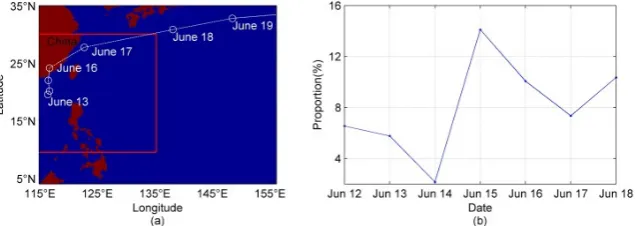
Figure 1 (a) The study area (10°N–30°N, 115°E–135°E) in red rectangle region and the track of the tropical storm
Hagibis labeled by day. The red and blue areas in (a) show land and ocean, respectively. (b) The coverage of SST
samples in the study region during the period from June 12 to June 18, 2014.
3. Methodology
3.1. RBFN method
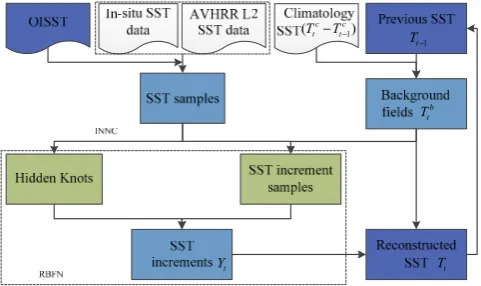
The daily SST can be considered as two parts: the background field and the SST increment[6, 26]. The previous SST field is used as the background field. In particular, the values of climatology change are added to the background field. The reconstructed SST Tt can be defined as
-1 ( 1)
b t t t
b c c
t t t t
T Y T
T T T T−
= +
= + −
(1)
where Yt is the SST increment, b t
T is the background field, and Tt-1 is the reconstructed SST for
the previous time. For convenience, we use the OISST product as the a priori SST, and to minimize the effects of this, the procedure was run for 10 days in advance of the first date. The daily SST climatology, Ttc, was obtained from 30 years (1982–2011) of OISST data[27]. ( 1)
c c
t t
T −T− is the SST climatology that changes between time t and t–1. The SST increment Yt is calculated from the RBFN
proposed by Ryu et al.[24]. It should be noted that this RBFN is used to estimate SST increments, not SSTs as in Ryu’s et al. study. The RBFN can be given by
,0 , 1 , , 5
( )
( ) t ( )
t t t
K d T
t t t t m k t k t k
Y f X
f X X z
ε
β
β
=φ
β
+ = + = + +
(2)where f X( t) is a RBFN function, Xt =(X Xt1, t2) is a 2-dimensional vector, and X Xt1, t2 are the
longitude and latitude at time t, respectively. Xtd denotes the set of all possible power with d
degree. Here, d = 2 and the 2-degree polynomial can be expressed as (1, 1, 2, 1 2, 21, 22) d
t t t t t t t
X = X X X X X X
. zt k, = Xt −μt k, denotes the distance between Xt and hidden knots ut k, for k=1,...,Kt, and ( )z z
φ = . βt,0 , βt m, , m=1,...,5; and βt k, +5 denote regression coefficients for the intercept,
polynomials, and basis functions, respectively.
ε
t is an independent Gaussian random error withmean 0 and variance σ2yt.
Using this RBFN method, the number of hidden knots Kt, the position, and error variance are
unknown, and are strongly related to the precision of the reconstructed SST. The error variance is estimated by the squared deviation of the difference between f X( t) and SST increments Yt. Since
t Y
1 t T−
b t T
t T 1
( c c)
t t
T −T−
Figure 2 Schematic diagram of the RBFN method for reconstructing SST.
3.2. INNC algorithm
The nearest neighbor cluster (NNC) algorithm is used to search the optimal hidden knots only from the SST samples for RBFNs[28, 29], while the INNC algorithm choose the hidden knots from both SST samples and background field, and consider the values of SST samples. The INNC algorithm is described as follows.
(1) Standardizing the original SST data, and make sure each variable of (x y z, , ) in the SST matrix with the mean of 0 and standard deviation of 1, where z is the value of the SST at the position of (x y, ) in the SST matrix.
(2) Define a minimal distance D and set the first SST sample (x y z1, 1, 1) as the first center
c
1.
(3) For the second SST sample ( , , )x y z2 2 2 , the Euclidean distance s to the center c1 is
calculated. If s > D, then the position ( , , )x y z2 2 2 is the next center c2, otherwise the
algorithm searches for the next SST sample ( , , )x y z3 3 3 .
(4) For the i-th SST sample ( , , )x y zi i i , the Euclidean distance
{ }
sk to each center{ }
ck iscalculated, k=1,…,K. K is the number of center. If the minimal distance sm >D, then the
position ( , , )x y zi i i is the next center cK+1, otherwise the algorithm searches for the next
SST sample, until the last one is found.
(5) The values from the background field Ttb are used to fill the positions without SST
samples, before repeating step (3) for each position to select the centers from the background field. This continues until all the positions are processed in the SST matrix, and the hidden knots ut are obtained by using the positions of centers
{ }
ck in the SSTmatrix.
In terms of the INNC algorithm, the parameters Kt and ut are determined when the minimal
distance D is defined. The value of D ranges from 0.2 to 1.5 in this study, and the optimal D is selected with the minimal error variance σy2t to obtain the optimal Kt and ut for RBFN. Thus,
the optimal Kt and ut may vary with different quantities and distributions of SST samples. In
addition, the SST values at the positions of the optimal hidden knots from the background fields are added to the SST samples, so there is at least one SST sample in the SST field within the minimal distance of D.
3.3. Evaluating the performance of the RBFN method
As described above, a simplified multi-quadric function z2+s12 (s1 equal 0 here) is chosen as
In order to evaluate the performance of this RBFN method, a Gaussian function exp(−s z2 2) is
selected for comparison and s2=K dt max [30], because dmax is the maximum distance between the
hidden knots, thus dmax =D in the study. And K-means algorithm and Kohonen-map algorithm are
also tested for selecting hidden knots for RBFNs. While the number of hidden knots Kt should be assigned for these two clustering algorithms, so the value of Kt ranges from 20 to 120 for K-means
algorithm, and the Kohonen-maps with regular array of m m× hidden knots are tested and the value of m ranges from 5 to 15, then the optimal values of Kt and m are separately selected with the minimal error variance σy2t. More Details about K-means algorithm and Kohonen-map algorithm
are described in [31-33].
Additionally, the OI method is used to compare with this RBFN method. Since the values of SST samples are assigned by the reference SST in the study, we select the noise-to-signal standard deviation ratio of AVHRR data for SST samples (the value is 0.5) and the average correlation scales for OI method (zonal and meridional correlation scales are 151 km and 155 km, respectively). Details of the OI method are described by Reynolds et al.[6].
To validate the accuracy of SST, the reconstructed SSTs are compared with the reference SSTs, and four commonly used error metrics are calculated: root mean square error (RMSE), mean absolute error (MAE), Pearson correlation coefficient (R), and signal-to-noise ratio (SNR). The SNR is the ratio of the standard deviation of the SST results to the standard deviation of the errors[34].
4. Results
In this section, the RBFN methods with different basis functions and clustering methods are tested, and the performance of the RBFN method for reconstructing daily SSTs is evaluated by comparing with the OI method.
4.1. Results from different basis functions
Using the INNC algorithm, the optimal hidden knots can be chosen from SST samples and background fields. But the distributions of SST samples are very sparse in this study, the reconstructed SSTs from the RBFN method may be influenced by the type of the basis function.
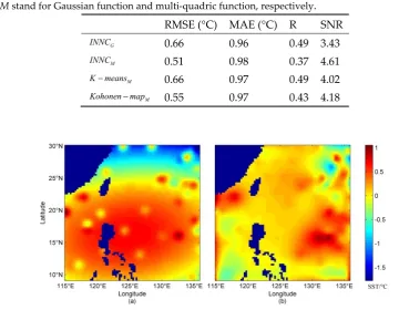
Figs. 3 and 4 display the SST increments estimated by using equation (2) with Gaussian function and multi-quadric function on June 13 and June 18 respectively. It is clear that the SST increments obtained from Gaussian function have a lot of anomaly circular regions as shown in Figs. 3(a) and 4(a), where the SST increments are significant different to the values from the regions behind them. While the SST increment fields using multi-quadric function in Figs. 3(b) and 4(b) are quite close to their neighborhood regions. Besides, due to the characteristics of Gaussian function, the effective areas of the hidden knots are limited, so the SST increments are strongly affected by the hidden knots that selected from the background fields when there are few SST samples nearby, which may cause large errors on SST increments.
Figure 3 Reconstructed SST increments on June 13, 2014 obtained by using (a) Gaussian function and (b)
multi-quadric function.
Table 1 Statistical results from different basis functions and clustering methods on June 13, 2014. the subscripts
G and M stand for Gaussian function and multi-quadric function, respectively. RMSE (°C) MAE (°C) R SNR
G INNC
0.66 0.96 0.49 3.43
M
INNC 0.51 0.98 0.37 4.61 M
K means− 0.66 0.97 0.49 4.02
M Kohonen map−
0.55 0.97 0.43 4.18
Figure 4 Reconstructed SST increments on June 18, 2014 obtained by using (a) Gaussian function and (b)
multi-quadric function.
Table 2 Statistical results from different basis functions and clustering methods on June 18, 2014. the subscripts
G and M stand for Gaussian function and multi-quadric function, respectively.
RMSE (°C) MAE (°C) R SNR
G INNC
0.73 0.97 0.52 3.60
M
INNC 0.47 0.98 0.34 4.64 M
K means− 0.59 0.97 0.43 4.06
M
4.2. Results from different clustering algorithms
A RBFN with too many or too few hidden knots is not conductive to simulating SST fields. Additionally, the distribution of hidden knots has a strong influence on the construction of a RBFN. Therefore, the quality of reconstructed SSTs from the RBFN method is highly related to the quantity and distribution of hidden knots, and it is important to select the suitable hidden knots for RBFNs.
Three clustering algorithm including K-means algorithm, Kohonen-map algorithm and INNC algorithm are compared to selecting the optimal hidden knots for RBFNs on June 13 and June 18, respectively. Since the RBFN is quite sensitive to the hidden knots, the values of hidden knots are very important to the reconstructed SSTs. As a result, if a hidden knot is obtained from the background field, the value of which is close to 0 in the SST increment field in equation (2), and the SST accuracy will decrease in this situation. Thus it is conductive to select the hidden knots from the SST samples rather than from the background field.
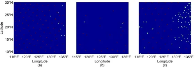
Figs 5 and 6 show the distributions of hidden knots from these three algorithms. It is easy to discover that there are more hidden knots are selected from the SST samples (green points) by the INNC algorithm than those by the other two algorithms, because the clustering centers of the K-means algorithm and the Kohonen-map algorithm are chosen by training the input samples, while the INNC algorithm directly select the hidden knots from the SST samples and make sure that as many hidden knots as possible are obtained from SST samples within the minimal distance
D. As the statistical results shown in Table 1 and 2, the INNC algorithm in this study with the highest accuracy of reconstructed SSTs, is more suitable than the K-means algorithm and the Kohonen-map algorithm to select the optimal hidden knots for the RBFN method.
Figure 5 The distributions of hidden knots for RBFN on June 13, 2014 from (a) K-means algorithm, (b)
Kohonen-map algorithm and (c) INNC algorithm respectively. The red points and green points are the
locations of hidden knots for RBFNs separately selected from the background field and the SST samples.
Due to the limitation of the correlation scales for the OI method, the SST increments will close to 0 when there are no SST samples behind them, while the SST increments from the RBFN method are obtained based on the tendency of the whole SST increment field. This is the key difference between the OI method and the RBFN method for reconstructing SST.
Figure 7 displays the time-series of each error metric from the OI and RBFN methods during the period from June 12 to June 18, 2014. The performance of each error metric from the RBFN method is much better than that from the OI method. The average values of these error metrics in Table 3 indicate that the RBFN method increases R and SNR from 0.96 and 3.82 to 0.98 and 4.94, respectively, and decreases RMSE and MAE from 0.69°C and 0.46°C to 0.48°C and 0.35°C, respectively. Although the RBFN method requires more computation time than the OI method, due to the selection of optimal hidden knots by using the INNC algorithm, the RBFN method has a better accuracy of reconstruction than the OI method.
In Figs. 8 and 9, the reconstructed SSTs from June 13 and June 18 are separately displayed as examples. The results show that the reconstructed SSTs from the OI method (shown in Figs. 8(b) and 9(b)) and the RBFN method (shown in Figs. 8(d) and 9(d)) are quite similar to their reference SSTs (see Figure 8(c) and 9(c)). But the SSTs in the region outlined by the square from the OI method have significantly high SST anomaly, where these phenomenon are not obvious in the SSTs from the RBFN method and their reference data. This indicates that the RBFN method has a relatively better performance than the OI method to reconstruct SSTs when the original SST samples is quite sparse as shown in Figs 8(a) and 9(a).
Figure 7 (a) RMSEs, (b) MAEs, (c) Rs and (d) SNRs of the reconstructed SSTs from the OI and RBFN methods in the study region during the period from June 12 to June 18, 2014.
Table 3 Statistical results from the OI and RBFN methods
Figure 8 The distributions of (a) original SST samples, (b) OI SST, (c) reference SST and (d) RBFN SST on June
13, 2014. The region outlined by the square is used for comparison in detail.
Figure 9 The distributions of (a) original SST samples, (b) OI SST, (c) reference SST and (d)RBFN SST on June
18, 2014. The region outlined by the square is used for comparison in detail.
5. Disccusion
5.1 The INCC algorithm for RBFNs
The hidden knots for RBFNs are commonly selected by clustering algorithms[28, 29, 35] or random sampling[24]. Since the hidden knots with different quantities and distributions should be tested in RBFNs, huge computational resources are required when random sampling is used to select the optimal hidden knots from SST fields. Commonly used clustering algorithms for RBFNs, such as K-means algorithm and Kohonen-map algorithm, are only used to determine the distribution of hidden knots when the number of hidden knots is given[32, 35]. The K-means algorithm should be executed hundreds of times, which also takes a lot of time even though the algorithm has a fast convergence speed. For the Kohonen-map algorithm, an input vector is not only relate to the nearest hidden knot but also to its neighbor hidden knots, so the computation is also huge and the training step for the clustering centers consume a lot of time before the iteration ends .While using the INNC algorithm with a parameter D, both the quantity and distribution of hidden knots could be directly determined without any iterative computation, and the values of D in this study were chosen from 0.2 to 1.5. Thus, the INNC algorithm is more efficient in selecting the optimal hidden knots for RBFNs.
The coverage of SST samples we selected in the study is very low because the tropical storm Hagibis come with heavy clouds, which makes poor quality of satellite-retrieved SSTs, and the SSTs we can used are very limited. Theoretically, the errors of reconstructed SSTs are from both background fields and SST increments. The SST increments are estimated by using current SST samples, and the quality of background fields is strongly influenced by the previous SST samples, thus the distributions of SST samples at both the previous time and the current time play a significant role in reconstructing SST. It can well explain the fact that the minimal RMSE didn’t happened on June 15 in Figure 7(a), which has the highest coverage of SST samples as shown in Figure 1(b). Because the June 14 with the lowest SST coverage in the study has a low accuracy of reconstructed SST, and make a poor quality of the background field for June 15, so the accuracy of reconstructed SST on June 15 is not the best even though it has the highest coverage of SST samples.
The quality of SST samples is not only relevant to the coverage of SST samples, but also depends on their accuracy. Since the SST sample values used were assigned by the reference SSTs, which can be considered as non-biased SST data, the reconstructed SSTs are of relatively high quality. However, the satellite-retrieved SST is often contaminated by the atmosphere and the SST data from different sources may contain errors from their respective surveying systems, meaning it is not easy to obtain non-biased SST data, and the accuracy will decrease if large errors exist in SST samples.
The SST samples with high coverage are conductive to acquiring high-quality daily SSTs. While acquiring larger quantities of SST samples often need to combine different sources of SSTs. However, more SST errors may come from these different kinds of sensors, and this has a negative influence on the quality of the SST samples overall. For the purpose of obtaining high-accuracy SST data from the RBFN method, more SST data should be used in reconstructing the SST. Additionally, strict quality control is required for SSTs from various measurements, and bias corrections for satellite-retrieved SSTs are necessary to eliminate the errors in SST samples.
5.3 The performance of the RBFN method
Since the OI method estimates SSTs using only the information within a limited distance, the estimated SSTs in some areas rely on background fields, which create large errors in the SST fields. The RBFNs with enough hidden knots use all the SST samples to approximate the SST field, so the SSTs from the RBFN method contain more information on the whole SST field, not only the information about SST samples nearby. Thus, the accuracy of SST obtained using the RBFN method is better than that using the OI method when the distribution of SST samples is quite sparse.
As shown in Figure 7(a), the RMSE on June 15 from the RBFN method is quite smaller than that from the OI method when the quality of the background field is quite poor. This shows that compared with the SSTs from the OI method, the quality of SSTs from the RBFN method is more stable when the SST errors are associated with the background field.
On the other hand, the OI method is effective in estimating SST using neighboring samples, which was conductive to obtaining a higher accuracy of SSTs when the coverage of the SST samples is very high. While the quantity and distribution of hidden knots in RBFNs are determined by the minimal error variance , which is a global variable of the SST field, and the distribution of hidden knots may not be suitable in some local regions and the SST errors of RBFNs may occur even in some areas with large amount of SST samples nearby.
but the RBFN method is more effective than the OI method when the SST samples are sparsely distributed.
6. Conclution
Reconstructing SST fields from a limited number of SST samples is important for data applications. In this study, a RBFN method is proposed and a INNC algorithm is designed to search the optimal hidden knots for RBFNs. Compared with the other clustering algorithms as K-means algorithm and Kohonen-map algorithm, the INNC algorithm can obtain more hidden knots from the SST samples, which will contribute to acquiring high quality of reconstructed SST. And using the multi-quadric function as basis function is more effective than the Gaussian function to avoid the SST increment anomaly on the regions of hidden knots. Thus the INNC algorithm with multi-quadric function is quite suitable for the RBFN method to reconstruct SSTs in the study.
To evaluate the accuracy of this RBFN method, SST samples with low coverages are reconstructed by using the RBFN and OI methods, respectively. The results show that compared with the SSTs from the OI method, the quality of SST from the RBFN method is more stable when the SST errors are associated with the background field. Moreover, the RBFN method is less affected by missing values in SST samples, and the SSTs from the RBFN method have a higher accuracy than those from the OI method when SST samples are sparsely distributed.
Considering the efficiency of RBFNs, hidden knots with different quantities and distributions are determined simultaneously using various D values in the INCC algorithm, and the optimal D for RBFN is selected with the minimal error variance. The step-length of D is set as 0.02 in this study. And we believe that if the step-length of D can be set smaller, the accuracy may be improved.
However, the accuracy of reconstructed SSTs is strongly influenced by the quality of SST samples from both the present and current time, and the biases in SST samples will increase the errors in SSTs, thus the strict quality control and bias corrections to SST samples are required in practice.
Acknowledgments: The authors thank NESDIS/STAR, NOAA/NCDC and NSMC of China for providing the in-situ and SST products in the study. This work was supported by the National Natural Science Foundation of China (No.41476154, No.41371385 and No.41671401) and the National key research and development program of China (No.2016YFA0600304).
Conflicts of Interest: The authors declare no conflict of interest.
References
1. Saha, S., et al., The NCEP climate forecast system version 2. Journal of Climate, 2014. 27(6): p.
2185-2208.
2. Shirvani, A., S. Nazemosadat, and E. Kahya, Analyses of the Persian Gulf sea surface temperature:
prediction and detection of climate change signals. Arabian Journal of Geosciences, 2015. 8(4): p.
2121-2130.
3. Knutson, T.R., et al., Tropical cyclones and climate change. Nature Geoscience, 2010. 3(3): p. 157-163.
4. Donlon, C., et al., The global ocean data assimilation experiment high-resolution sea surface
temperature pilot project. Bulletin of the American Meteorological Society, 2007. 88(8): p. 1197-1213.
5. Martin, M., et al., Group for High Resolution Sea Surface temperature (GHRSST) analysis fields
inter-comparisons. Part 1: A GHRSST multi-product ensemble (GMPE). Deep Sea Research Part II:
Topical Studies in Oceanography, 2012. 77: p. 21-30.
6. Reynolds, R.W., et al., Daily high-resolution-blended analyses for sea surface temperature. Journal of
75-87.
8. Smith, T.M., et al., Reconstruction of historical sea surface temperatures using empirical orthogonal
functions. Journal of Climate, 1996. 9(6): p. 1403-1420.
9. Smith, T.M., R.E. Livezey, and S.S. Shen, An improved method for analyzing sparse and irregularly
distributed SST data on a regular grid: The tropical Pacific Ocean. Journal of climate, 1998. 11(7): p.
1717-1729.
10. Ping, B., F. Su, and Y. Meng, Reconstruction of Satellite-Derived Sea Surface Temperature Data Based
on an Improved DINEOF Algorithm. Selected Topics in Applied Earth Observations and Remote
Sensing, IEEE Journal of, 2015. 8(8): p. 4181-4188.
11. Beckers, J.-M. and M. Rixen, EOF Calculations and Data Filling from Incomplete Oceanographic
Datasets*. Journal of Atmospheric and Oceanic Technology, 2003. 20(12): p. 1839-1856.
12. Beggs, H., et al., RAMSSA—An operational, high-resolution, Regional Australian Multi-Sensor Sea
surface temperature Analysis over the Australian region. Australian Meteorological and
Oceanographic Journal, 2011. 61(1): p. 1.
13. Brasnett, B., The impact of satellite retrievals in a global sea-surface-temperature analysis. Quarterly
Journal of the Royal Meteorological Society, 2008. 134(636): p. 1745-1760.
14. Cummings, J.A., Operational multivariate ocean data assimilation. Quarterly Journal of the Royal
Meteorological Society, 2005. 131(613): p. 3583-3604.
15. Donlon, C.J., et al., The operational sea surface temperature and sea ice analysis (OSTIA) system.
Remote Sensing of Environment, 2012. 116: p. 140-158.
16. Gemmill, W., B. Katz, and X. Li, Daily real-time global sea surface temperature—high-resolution
analysis: RTG_SST_HR. NCEP. 2007, EMC Office Note.
17. Gentemann, C.L., F.J. Wentz, and M. DeMaria. Near real time global optimum interpolated microwave
SSTs: Applications to hurricane intensity forecasting. in 27th conference on hurricanes and tropical
meteorology, Monterey, CA. 2006.
18. Park, J. and I.W. Sandberg, Universal approximation using radial-basis-function networks. Neural
computation, 1991. 3(2): p. 246-257.
19. Holmes, C. and B. Mallick, Bayesian radial basis functions of variable dimension. Neural computation,
1998. 10(5): p. 1217-1233.
20. Powell, J. Radial basis function approximations to polynomials. in Numerical analysis 1987. 1989.
Longman Publishing Group.
21. Liu, L., L. Chua, and D. Ghista, Mesh-free radial basis function method for static, free vibration and
buckling analysis of shear deformable composite laminates. Composite Structures, 2007. 78(1): p.
58-69.
22. Miazhynskaia, T., S. Frühwirth-Schnatter, and G. Dorffner, Neural network models for conditional
distribution under bayesian analysis. Neural computation, 2008. 20(2): p. 504-522.
23. Konishi, S., T. Ando, and S. Imoto, Bayesian information criteria and smoothing parameter selection in
radial basis function networks. Biometrika, 2004. 91(1): p. 27-43.
24. Ryu, D., F. Liang, and B.K. Mallick, Sea surface temperature modeling using radial basis function
networks with a dynamically weighted particle filter. Journal of the American Statistical Association,
25. Xu, F. and A. Ignatov, In situ SST quality monitor (i quam). Journal of Atmospheric and Oceanic
Technology, 2014. 31(1): p. 164-180.
26. Reynolds, R.W. and T.M. Smith, Improved global sea surface temperature analyses using optimum
interpolation. Journal of climate, 1994. 7(6): p. 929-948.
27. Banzon, V.F., et al., A 1/4°-Spatial-Resolution Daily Sea Surface Temperature Climatology Based on a
Blended Satellite and in situ Analysis. Journal of Climate, 2014. 27(21): p. 8221-8228.
28. XiaoHua, D. Study on regional financial risk early warning system based on uniform design method
and Nearest Neighbo-Clustering RBFNN. in Conference Anthology, IEEE. 2013. IEEE.
29. Zhu, M. and D. Zhang, Study on the Algorithms of Selecting the Radial Basis Function Center. Journal
of Anhui University, 2000. 3: p. 72-78.
30. Lowe, D. Adaptive radial basis function nonlinearities, and the problem of generalisation. in Artificial
Neural Networks, 1989., First IEE International Conference on (Conf. Publ. No. 313). 1989.
31. Kanungo, T., et al., An efficient k-means clustering algorithm: analysis and implementation. IEEE
Transactions on Pattern Analysis and Machine Intelligence, 2002. 24(7): p. 881-892.
32. Latif, B.A., et al., Preprocessing of Low-Resolution Time Series Contaminated by Clouds and Shadows.
IEEE Transactions on Geoscience and Remote Sensing, 2008. 46(7): p. 2083-2096.
33. Kohonen, T., The self-organizing map. Proceedings of the IEEE, 1990. 78(9): p. 1464-1480.
34. Zhang, H., et al., Using residual resampling and sensitivity analysis to improve particle filter data