Using the MCNP Taylor series perturbation feature (efficiently) for shielding problems

*

Corresponding author: [email protected]

Using the MCNP Taylor series perturbation feature (efficiently)

for shielding problems

Jeffrey Favorite*

X-Computational Physics Division, XCP-3, P.O. Box 1663 MS F663, Los Alamos National Laboratory, Los Alamos, NM 87545 USA

Abstract. The Taylor series or differential operator perturbation method, implemented in MCNP and invoked using the PERT card, can be used for efficient parameter studies in shielding problems. This paper shows how only two PERT cards are needed to generate an entire parameter study, including statistical uncertainty estimates (an additional three PERT cards can be used to give exact statistical uncertainties). One realistic example problem involves a detailed helium-3 neutron detector model and its efficiency as a function of the density of its high-density polyethylene moderator. The MCNP differential operator perturbation capability is extremely accurate for this problem. A second problem involves the density of the polyethylene reflector of the BeRP ball and is an example of first-order sensitivity analysis using the PERT capability. A third problem is an analytic verification of the PERT capability.

1 Introduction

The Taylor series or differential operator perturbation feature [1, 2] was introduced into MCNP [3] in version 4B in the mid-1990s. The perturbation feature has been shown to be unreliable for estimating perturbations in eigenvalue (keff) problems [4, 5]. However, for fixed-source (shielding) problems, the perturbation feature can be extremely accurate and deserves to be more widely used. The Taylor series perturbation feature is invoked with the PERT card.

In publications until now [e.g., 2], a separate MCNP PERT card was used for each perturbed point in a parameter study. In fact, the MCNP manual [3] recommends two PERT cards for each perturbation so that the first- and second-order Taylor terms can be examined independently. The manual says that “each perturbation increases running time by 10%-20%” [3]. Limiting the number of PERT cards is therefore desirable.

This paper shows how to compute the two coefficients of a two-term Taylor expansion using only two PERT cards. These coefficients can then be used to estimate the perturbed response for any point in a parameter study. The statistical uncertainty can be well estimated from these two PERT cards; it can be computed exactly using three more PERT cards.

In addition, this paper shows how to use the PERT card to perform first-order sensitivity analysis such as may be used in uncertainty quantification.

We emphasize that the results of this paper apply only to fixed-source problems, not eigenvalue problems.

2 Taylor series coefficients

A Taylor series expansion of a response c that is a function of some reaction cross section Vx is

, ) ( 2

1 )

( )

( 2

2 2 0

,

0 , 0

,

'

'

x

x x x x x

x

x d

c d d

dc c

c V

V V V V V

V V

where Vx,0 is the reference value of the cross section and

.

0 ,

x x

x V V

V { '

Define the first- and second-order Taylor series terms as

x x _x

d dc

c V

V V ' {

'

0 ,

1

and

, ) ( 2

1 2

2 2 2

0 ,

x x x d

c d

c V

V _V '

{ '

respectively. Define px as the relative cross-section

change,

.

0 ,

x x x

p

VV

' {

Then, using the chain rule, the Taylor series terms can be written conveniently as

x p x

p dp

dc c

x 0

1

'

and

. 2

1 2

0 2 2

2 x

p x

p dp

c d c

x

'

For notational convenience, define c₀{c(V_x,0).

(1)

(2)

(3)

(4)

(5)

(6)

3 Taylor series coefficients and the

MCNP PERT card

3.1 Computing the coefficients

At present, the MCNP perturbation capability, invoked with the PERT card, uses a two-term Taylor expansion with no cross terms [6, 3]. The perturbation feature estimates the derivatives in Eqs. (6) and (7) and multiplies them by the relative perturbation px (or

2

x

p ) computed from the user input.

Define coefficients 0 1 { x p x dp dc c and . 2 1 0 2 2 2 { x p x dp c d c

These coefficients can be computed from any single arbitrary reference perturbation amount px,r using, from

Eqs. (6) and (7),

r x r x p p c c , , 1 1 ) ( ' and . ) ( 2 , , 2 2 r x r x p p c c '

Now the perturbed response due to an arbitrary perturbation px can be computed using

. ) ( 2 2 1 0

PERT px c cpx c px

c

Equation (12) [with Eqs. (10) and (11)] is the main conclusion of this paper. With this equation, a parameter study can be done for any number of perturbed values of the parameter with only two MCNP PERT cards, rather than the two PERT cards per perturbation that are recommended in the manual. A detailed prescription is given in Sec. 4.

3.2 Approximate uncertainty

The standard deviations of the Monte Carlo estimates of

1

c and c2, sc₁ and sc2, are

r x c c p s s , 1 1 ' and , 2 , 2 2 r x c c p s s '

where s_'c1 and s_'c2 are the standard deviations of the Monte Carlo estimates of 'c1 and 'c2 [meaning

)

( ,

1 pxr

c

' and 'c2(px,r) here and in the rest of this paper].

The standard deviation of the unperturbed tally c0 is sc0. With these quantities, the variance of the estimated perturbed tally of Eq. (12), estimated by assuming that

0

c, 'c1, and 'c2 are uncorrelated (subscript “unc.”), is

. 4 2 2 2 2 2 2 1 0 . ,

PERT c c x c x

c s s p s p

s

unc

3.3 Exact uncertainty

Typically, and in the prescription given in Sec. 4, c0, 'c1,

and 'c2 are all computed from the same set of histories

in the same cells. They are likely to be highly correlated. The effect of the correlations among c0, 'c1, and 'c2 on

the variance 2 PERT

c

s can be computed exactly.

The covariance matrix for cPERT is

, 2 2 2 1 2 1 2 0 2 1 1 1 0 2 0 1 0 0 » » » ¼ º « « « ¬ ª ' ' ' ' ' ' ' ' ' ' c c c c c c c c c c c c c c c s s s C U U U U U U

where the covariances are ,

y x xy xy{r ss

U

where the correlation coefficients are

>

( )

@

>

@

,

2 2 2 2

¦

¦

¦

¦

¦

¦

¦

{ i i i i i i i i xy y y N x x N y x y x N r

where N is the number of histories sampled and xi and yi are the x and y scores for the ith history.

We now find the correlation coefficient r_xy in terms of x, y, and z, where z = x + y. The variance in a Monte Carlo estimate of z, implicitly accounting for correlations in x and y, is

>

2

@

.

1 ) ( 2 1 ) ( 1 ) ( 1 1 1 2 2 3 2 2 2 2 3 2 2 2 3 2 2 2

¦

¦

¦

¦

¦

¦

¦

¦

¦

¦

¦

i i i i i i i i i i i i i i z y x y x N y x y x N y x N y x N z N z N s

The variance in a Monte Carlo estimate of the sum x + y,

not accounting for correlations in x and y, is

1

>

@

.

1 2 2

3 2 2 2 2 2 2

¦

¦

¦

¦

i i i i y x y x y x N y x N s s s

Using Eq. (20) in Eq. (19) yields

>

( )

@

.

2 3 2 2

¦

¦

¦

y i i i i

x

z N x y x y

N s s

Rearranging Eq. (21) and using the result in Eq. (18) [with the first line of Eq. (19), replacing z with x and y] yields

, 2 2 2 2 2 3 2 3 2 2 3 y x y x z y x y x z xy s s s s s N s N s s N r

. 2 2 2 2 y x y x z xy s s s s s r

Equation (23) will be applied for (x,y)(c0,'c1,'c2) and z(c0'c1,c0'c2,'c1'c2). Using Eq. (23) in Eq. (17) yields

).

( 2 2 2

2 1

y x z xy s s s U

The sensitivity vector for cPERT [from Eq. (12) with

Eqs. (10) and (11)] is

. , , 1 , , 2 , , 2 PERT 1 PERT 0 PERT T r x x r x x T p p p p c c c c c c S » » ¼ º « « ¬ ª ¸ ¸ ¹ · ¨ ¨ © § » ¼ º « ¬ ª ' w w ' w w w w

where superscript T indicates the transpose.

Using the “sandwich rule,” the total variance in cPERT

is

.

2

PERT S C S

sc T

Using Eqs. (15), (16), (24), and (25), Eq. (26) becomes

. 3 , 2 2 2 2 , 2 2 2 , 2 2 2 2 2 2 1 2 1 2 0 2 0 1 0 1 0 . , PERT PERT ¸ ¸ ¹ · ¨ ¨ © § ¸ ¸ ¹ · ¨ ¨ © § ¸ ¸ ¹ · ¨ ¨ © § ' ' ' ' ' ' ' ' r x x c c c c r x x c c c c r x x c c c c c c p p s s s p p s s s p p s s s s s _unc

4 Prescription for perturbations

4.1 Basic

The prescription to estimate a response c for any number of perturbations of a parameter px is as follows:

Choose a reference perturbation p_x,r; a convenient choice is p_x,r 1.

Set up two PERT cards with the density equal to [from Eqs. (2) and (5)] V_x,r V_x,0(1p_x,r). Obviously, if

1

,r x

p , then Vx,r 2Vx,0. One PERT card uses

METHOD = 2 and the other uses METHOD = 3. Run the problem using MCNP.

The METHOD = 2 perturbation result is 'c₁(p_x,r) ±

1

c

s_' ; use Eq. (10) to compute c1. The METHOD = 3

perturbation result is 'c₂(p_x,r) ± s'c₂; use Eq. (11) to

compute c2. Compute the standard deviations using Eqs.

(13) and (14).

A practically continuous curve of cPERT(px) can now be created using Eq. (12) with uncertainties estimated using Eq. (15).

4.2 Checking accuracy

As stated in the manual, it is a good idea to test whether a second-order Taylor expansion is accurate for the largest perturbation that is expected. One way to do this is to compare the first- and second-order terms c1px and

2 2px

c with the total cPERT(px), as suggested in the manual. This can be done for all values of p_x used in the analysis without additional PERT cards. From Eq. (12), the ratio of the second-order term to the first-order term is , 1st 2nd 1 2 1 2 2 x x x _p c c p c p c

which is linear with the relative perturbation.

However, contrary to statements in the manual, it is not always true that the second-order term should contribute much less to the total than the first-order term. For example, consider the notional curve shown in Fig. 1. The base case of V0 = 2 is at or near the optimum for

response R. The first-order Taylor term is zero or close to zero, and the second-order term dominates. Higher-order terms may be zero. Caution is advised.

Where possible, it is wise to use a direct calculation of the perturbed tally to test cPERT(px) for the maximum values of r px that are of interest.

4.3 Exact uncertainty

Exact uncertainties that account for the correlations among c0, 'c1, and 'c2 can be computed as follows:

Set up three more PERT cards in addition to those set up in Sec. 4.1 (with the same density as in Sec. 4.1). One of the new PERT cards uses METHOD = –2, one uses METHOD = –3, and one uses METHOD = 1.

Run the problem using MCNP.

The METHOD = –2 perturbation result is )

( _,

1 0 c pxr

c ' ±

1 0 c

c

s _' . The METHOD = –3 perturbation

result is c₀'c₂(p_x,r) ± sc₀'c₂. The METHOD = 1

perturbation result is 'c1(px,r)'c2(px,r) ± s'c1'c2. (23) (24) (25) (26) (27) (28)

Fig. 1. Notional graph of a response R as a function of a

Exact uncertainties may now be computed using Eqs. (15) and (27). Note that the perturbation results for METHOD = –2, –3, and 1 are not used; only the corresponding uncertainties are used.

5 Prescription for first-order sensitivity

analysis

5.1 Basic

The first-order relative sensitivity coefficient of a response c to some reaction cross section V_x is defined as

.

0 ,

0 0 , ,

x x

x x c

d dc c S

V

V {V _V

Using V_x V_x,0(1p_x) in Eq. (29) with the chain rule yields

, 1

0 0 ,

x x

p x c

dp dc c S _V

or, from Eq. (8),

.

0 1 ,

c c S

x

cV

The prescription to estimate the first-order sensitivity coefficient is now clear: Follow the prescription of Sec. 4.1 to compute c1, and divide the result by the

unperturbed response c0. The estimated variance of the

sensitivity coefficient, assuming c0 and c1 are

uncorrelated (subscript “unc.”), is

.

2

1 2

0 2

,

2 0 1

.

» » ¼ º «

« ¬ ª

¸¸ ¹ · ¨¨ © § ¸¸ ¹ · ¨¨ © §

c s c s S

s_{Sunc cVx} c c

Equation (13) gives sc₁. In this approximation, only

METHOD = 2 is required.

5.2 Exact uncertainty

The sensitivity vector for x c

S_,V [from Eq. (31) with Eq. (10)] is

. 1 , ,

0 , 2 0 ,

1 1 , 0 ,

T

r x r x

T c c

c p c p

c c S c S

S x x

» » ¼ º «

« ¬ ª '

» ¼ º «

¬ ª

' w w w

w V V

The covariance matrix for x c

S_,V is

,

2 2

1 1 0

1 0 0

» » ¼ º «

« ¬ ª

' '

'

c c c

c c c

s s C

U U

with

, )

( 2 2 2

2 1

1 0 1 0 1

0c c c c c

c' s ' s s'

U

as in Sec. 3.3. Using Eq. (26) (the sandwich rule) and Eqs. (31) and (32), the total variance of the sensitivity coefficient is

.

1 0

2 , 2 2 2 2 2

1 0 1 0

. ¸¸

¹ · ¨ ¨ © §

'

_{' '}

c c

S s s s s

s x

unc

c c c c c S S

V

In this case, as in Sec. 4.3, the METHOD = 2 result gives

1

c

s_' , and a PERT card with METHOD = –2 is

needed to give sc₀'c₁.

6 Numerical examples

6.1 Neutron detector polyethylene density

As an example, consider a detailed model of a neutron detector consisting of 15 helium-3 tubes with an active height of 15 in. (Fig. 2) and pressure of 10 atm. arranged in three rows in a high-density polyethylene (HDPE) moderator (Fig. 3). The nominal density of the HDPE is (29)

(30)

(31)

(32)

(33)

(34)

(35)

(36)

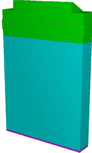
Fig. 2. Three-dimensional rendering of the neutron detector.

The light blue material is HDPE, within which are arranged the helium-3 tubes. The height of the HDPE is 16.59 in.

Fig. 3. Cross section of the neutron detector. The light blue

taken to be 0.962 g/cm3_{. How does the response of the}

detector change as the HDPE density changes?

An Am-Be source was modeled 30 cm from the front face of the detector and centered vertically with respect to the active height of the tubes. Detector counts were modeled as captures in helium-3 in the active part of the tubes.

The total efficiency as a function of HDPE density is plotted in Fig. 4. (The total efficiency is the number of counts per source particle emitted, and for this calculation it is not necessary to specify the source strength.) Seven direct calculations (using perturbed densities) as well as the unperturbed (reference) direct result are compared with a second-order Taylor series estimate computed using coefficients calculated during the run of the unperturbed reference case. Uncertainties for the Taylor series estimates are the uncorrelated estimates of Eq. (15). Figure 4 shows that the Taylor series estimate of the MCNP PERT card provides an extremely accurate and fast method for performing this sensitivity study.

Adding the two PERT cards increased the run time by 6%.

Including all correlations among the Taylor series coefficients changes the standard deviation from 4.67 × 10–6 _{to 4.43 × 10}–6 _{for the largest negative perturbation}

and from 4.42 × 10–6 _{to 4.49 × 10}–6 _{for the largest}

positive perturbation. Adding three more PERT cards increased the run time (from the case with two PERT cards) by only 5%.

The advantage of a continuous parameter study is not apparent in Fig. 4 since the direct results are relatively easy to acquire. However, another quantity of interest for the neutron detector is the “row ratio,” or the ratio of the sum of the counts in the second, third, fourth, and fifth tubes in the middle row (called row 2) to the sum of the counts in the two tubes in the back row (called row 3, the top row in Fig. 3).

Figure 5 shows the row ratio for the seven perturbed configurations and the unperturbed reference case. Statistical uncertainty causes “wiggle” in the curve through the points.

The Taylor series estimate, also shown on Fig. 5, was obtained as the ratio of the individual Taylor series estimates for the count rates for rows 2 and 3. Uncertainties for the Taylor series estimates use the uncorrelated estimate of Eq. (15) for each row.

Including all correlations among the Taylor series coefficients changes the standard deviation from 3.10 × 10–3 _{to 2.99 × 10}–3 _{for the largest negative perturbation}

and from 2.85 × 10–3 _{to 2.88 × 10}–3 _{for the largest}

positive perturbation.

Comparing the contributions of the first- and second-order terms, as suggested in the MCNP manual [3], can easily be done for each perturbed point using Eq. (12).

6.2 Neutron reflector polyethylene density

This problem illustrates the use of the PERT card for the sensitivity of a response to the mass density of a neutron reflector. The response is the total neutron leakage from a spherical system. The system is the polyethylene-reflected BeRP ball [7, 8] described in Table 1. The density of the polyethylene is perturbed.

The exact leakage for each perturbation is compared with the first- and second-order Taylor series perturbation estimates in Fig. 6. Error bars of one standard deviation are present but not visible. The second-order estimate of Eq. (12) produces the correct curvature near the unperturbed density (0.95 g/cm3_{), but}

it is too large for negative density perturbations and too small for positive density perturbations. A higher-order

Fig. 4. Efficiency for the neutron detector.

Fig. 5. Row ratio for the neutron detector.

Table 1. BeRP ball geometry and materials.

Material Outer Radius

(cm)

Density (g/cm3₎

-Pu 3.794 19.6

NO Gas Fill 3.82829 0.00129

Steel 3.85879 7.62

Taylor expansion is needed for more accuracy in the range of perturbations shown.

The error is quantified in Fig. 7 and presented with the ratio of the second-order term to the first-order term, as given by Eq. (28). For this problem, the error is within ±10% when the ratio is –0.40 to 0.33.

We turn now to the first-order sensitivity of the leakage to the polyethylene density, computed using Eq. (31). The first-order PERT method is compared with central-difference estimates computed using

, 2

) ( )

( _{0 0}

0 0

, ¸

¹ · ¨

©

§

|

h h c h c c SCD

c

U U

U

U

where h is the change made in the density to compute the central difference. It is important to choose the perturbation h small enough that the points c(U0h), c0,

and c(U₀h) are on a line but large enough that the difference c(U0h)c(U0h) can be calculated accurately [9], and, if a Monte Carlo code is used, with a small uncertainty. Central-difference estimates using Eq. (37) with different values of h and MCNP results for c

are shown in Table 2 with Monte Carlo relative uncertainties (1s). The difference between the PERT

estimate and the central-difference estimate is shown in terms of the number of standard deviations of difference.

The central-difference estimate using the smallest value of h (0.05 g/cm3_{) is just within 2s of the first-order}

PERT value of the sensitivity. Which is the more accurate value? The three points of the sensitivity are not exactly on a line: The Pearson correlation coefficient for the points is 0.9994. In our judgment, the PERT value is the most accurate.

6.3 Analytic monodirectional one-group slab

This problem applies the PERT card to the reaction rate inside a slab when there is a monodirectional source and no scattering. The solution is analytic, so this is a good verification problem for the PERT capability.

A boundary source of strength q impinges on the left, at x = 0 cm, and the width of the slab is X. The macroscopic cross section is . The flux ׋(x) at any point

x within the slab is

x

qe

x) 6

(

I

and the total reaction rate R within the slab is

1

. ) (

0 0

X

X _x

X

e q

qe dx

x dx R

6

6

6 6

³

³

I

The cross section is perturbed a relative amount p; in accordance with Eq. (5), we write the cross section as

). 1 (

0 p

6 6

Using Eq. (40) in Eq. (39), the reaction rate is

1 _e 0(1 p)X

.

q

R 6

From Eq. (41), the first derivative of R with respect to p is

.

) 1 ( 0

0 pX Xe q p

R ₆ 6

w w

The second derivative is

. )

( 2 (1 ) 0

2 2

0 pX e X q p

R ₆ 6

w w

The derivatives evaluated at p = 0 are

X

p

Xe q p

R ₀

0 0

6 6 w

w

Fig. 6. Neutron leakage as a function of BeRP polyethylene

density.

Fig. 7. Error in the second-order perturbation estimate and ratio

of second-order term to first-order term for the BeRP ball problem.

(37)

Table 2. Sensitivity of neutron leakage to polyethylene density.

Method h

(g/cm3₎

Sensitivity (%/%)

Diff. w.r.t. PERT (Ns)(a)

PERT N/A 0.9270 ± 0.23% N/A

Central Diff. 0.05 0.9370 ± 0.32% 1.94

Central Diff. 0.15 0.9949 ± 0.11% 20.7

Central Diff. 0.25 1.136 ± 0.07% 69.4 (a) Number of standard deviations of difference.

(38)

(39)

(40)

(41)

(42)

(43)

and

. )

( 2 0

0 0

2 2

X

p

e X q p

R ₆ 6

w w

The two-term Taylor series expansion is

, 2 1 )

(

2 2 1 0

2 0 2 2

0 0

p R p R R

p p

R p p R R p R

p p

TS

w w w w

where R1 and R2 are c1 and c2 of Eqs. (8) and (9).

We now apply the parameters of Table 3 to this problem. Analytic values of R0, R1, and R2 [from Eqs.

(41), (44), and (45), respectively] are shown in Table 4 and compared with values computed using MCNP. R0 is,

of course, a regular reaction-rate cell tally. R1 and R2

were computed using the PERT card as discussed in Sec. 4.1. The differences between the MCNP results and the analytic values are well within one standard deviation.

A parameter study is shown in Fig. 8. The exact reaction rate, from Eq. (41), is compared with the two-term Taylor series of Eq. (46) when the coefficients are computed analytically and when the coefficients are from the MCNP PERT capability. The two curves for the Taylor series are indistinguishable. Figure 8 shows that a two-term Taylor expansion is extremely accurate for cross-section perturbations of ±10% for this problem; beyond that, higher-order terms may be needed.

Figure 9 quantifies these observations, showing the error in the second-order PERT estimate as well as the ratio of the second- to the first-order Taylor term. For this problem, even when the second-order term is about

the same size as the first-order term, the error in the Taylor series estimate is less than 0.6%.

7 Summary and conclusions

The MCNP perturbation capability can be extremely accurate for shielding problems. This paper has demonstrated that it is not necessary to use a PERT card (or two PERT cards) for every perturbed point in a parameter study. Just two PERT cards suffice to obtain the Taylor series coefficients, generate a near-continuous curve of the resulting perturbed response, and estimate the statistical uncertainty in the perturbed response.

This paper has focused on cross-section and density perturbations. Material-substitution perturbations require special treatment [6], but it might be possible to apply the methods of this paper. On the other hand, the first- order sensitivity of a response to material composition changes can be computed using the first-order sensitivity to each of the individual nuclide densities, computed as described in Sec. 5. This topic is receiving new attention [10, 11].

(45)

(46)

Fig. 8. Exact reaction rate and Taylor series estimates for the

analytic problem.

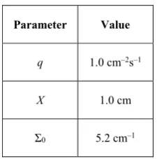
Table 3. Parameters of the analytic slab problem.

Parameter Value

q 1.0 cm–2_s–1

X 1.0 cm

0 5.2 cm–1

Table 4. Coefficients of the Taylor expansion.

Coefficient(a) _{Analytic MCNP PERT Ns}(b)

R0 (s–1) 0.994483 0.994428 ± 0.01% 0.57

R1 (s–1) 0.0286861 0.0287011 ± 0.83% 0.06

R2 (s–1) –0.0745840 –0.0746330 ± 0.48% 0.14

(a) The right side of Eq. (39) is multiplied by a unit area, making the units work out to s–1_.

(b) Number of standard deviations of difference.

Fig. 9. Error in the second-order perturbation estimate and ratio

The run times for the test problem of Sec. 6.1 increased by only ~20% of the rule of thumb quoted in the manual [3].

The PERT card must not be used to perturb problem parameters that would cause the source spatial, spectral, or angular distribution to be perturbed.

References

1. G. McKinney and E.T. Cheng, “MCNP Sensitivity Method Development and Applications,” Trans. Am. Nucl. Soc., 46, 278-279 (1984)

2. G.W. McKinney and J.L. Iverson, “Verification of the MCNP Perturbation Technique,” Proc. 1996 Top. Mtg. Rad. Prot. Shielding, Vol. 2, 959-966, No. Falmouth, Mass., April 21-25 (1996)

3. T. Goorley et al., “Initial MCNP6 Release Overview,” Nucl. Technol., 180, 298-315 (2012) 4. J.A. Favorite, “An Alternative Implementation of

the Differential Operator (Taylor Series) Perturbation Method for Monte Carlo Criticality Problems,” Nucl. Sci. Eng., 142, 327-341 (2002) 5. J.A. Favorite, “On the Accuracy of the Differential

Operator Monte Carlo Perturbation Method for Eigenvalue Problems,” Trans. Am. Nucl. Soc., 101, 460-462 (2009)

6. J.A. Favorite and D.K. Parsons, “Second-Order Cross Terms in Monte Carlo Differential Operator Perturbation Estimates,” Proc. Int. Conf.

Mathematical Methods for Nuclear Applications,

Salt Lake City, Utah, Sept. 9-13, CD-ROM (2001) 7. J. Mattingly, “Polyethylene-Reflected Plutonium

Metal Sphere: Subcritical Neutron and Gamma Measurements,” Sandia National Laboratories Report SAND2009-5804 Revision 3 (Rev. July 2012)

8. E.C. Miller et al., “Computational Evaluation of Neutron Multiplicity Measurements of Polyethylene-Reflected Plutonium Metal,” Nucl. Sci. Eng., 176, 167-185 (2014)

9. W.H. Press et al., Numerical Recipes in FORTRAN: The Art of Scientific Computing, 2nd _{ed., Chap. 5.7}

(reprinted with corrections) (Cambridge University Press, 1994)

10. J.A. Favorite et al., “Adjoint-Based Sensitivity and Uncertainty Analysis for Density and Composition: A User’s Guide,” Trans. Am. Nucl. Soc., 115, 669-672 (2016)