How to Increase Quality Measures of Software
Reliability prediction Using Fuzzy Logic
Shashi Prabha Anan
Department of Computer Science and Engineering
Kamla Nehru Institute of Technology, Sultanpur, Uttar Pradesh, India
Abstract— Recent years have witnessed a demand for software development era. In this paper presents a method to estimate the expected number of faults in the software in the early phase of its development and is based on the factors that influence software quality in the programming environment. The paper includes analysis of the five predicting variables and the required response variable to predict the early software reliability based on the previous data available. To predict the number of faults in the software before testing, data sets from previous projects are used. To evaluate the predictive capability of the developed model the predicted faults are compared with the actual faults. In this paper identifying the key influencing parameters are Techno-complexity, Practitioner level, Creation Effort, Review effort, Urgency.
Keywords— Faults, failure, defects, errors, estimation, prediction, quality metrics, etc.
1. INTRODUCTION
A software product can be released only after some pre-specified reliability criterion has been met at the end of the development cycle. In recent years, researchers have proposed a number of analytical models for early software reliability prediction. The problem of developing reliable software at low cost remains an open challenge. To develop a reliable software system, several issues are to be addressed. These include specification of reliable software, reliable development methodologies, testing methods for reliability, reliability growth prediction modeling, and accurate estimation of reliability. The issue of finding a common model for all possible software projects is yet to be solved. Selection of a particular model is very important in software reliability growth prediction because both the release date and the resource allocation decision can be affected by the accuracy of prediction.
1.1THE NEED FOR RELIABLE SOFTWARE
The dependence on computers in a person’s daily lives has been increased as computers are embedded in wristwatches, telephones, home appliances, buildings, automobiles, and aircraft. All the industries including automotive, avionics, oil, telecommunications, banking,
semiconductors, and pharmaceuticals- are highly dependent on computers for their basic functioning. The computer revolution is powered by an ever more rapid technological advancement. Science and technology demand high-performance hardware and high-quality software for making improvements.
The size and complexity of computer-intensive systems has grown dramatically during the past decade [10], and the trend will certainly continue in the future. Contemporary examples of highly complex hardware and software systems are the projects undertaken by NASA, the Department of Defense, the new generation air traffic control system, and a variety of other industries. In the offices and homes, personal computers cannot function without complex operating systems (e.g., Windows) ranging from 1 to 5million lines of code provide a variety of applications for our daily use of these computers. When the dependencies on computers increase, the possibility of crises from computer failures also increases since the demand for complex hardware and software systems has increased more rapidly than the ability to design, implement, test, and maintain them. The impact of these failures ranges from malfunctions of home appliances to economic damage (e.g., interruptions of banking systems) to loss of life (e-g., failures of flight systems or medical software). Therefore, assessing the reliability of computer systems has become a major concern for the society.
1.1.1 SOFTWARE RELIABILITY CONCEPTS Software Reliability as an important quality attribute highly valued by customers and users and has the most significant impact on the performance. Software Reliability metric is used to help the managers to guide software development. Software reliability can be formally defined as the probability of failure-free software operation in a specified environment for a specified period of time. A software failure occurs when the behavior of the software departs from its specifications, and it is the result of a software fault, a design defect, being activated by certain input to the code during its execution. Generally, a software failure caused by software faults latent in the system cannot occur except for a special occasion when a set of special data is put into the system under a special condition, i.e. the program path including software faults is executed. Therefore, the software reliability is dependent on the input data and the internal condition of the program. In software, an error is usually a programmer action or omission that results in a fault. A fault is a software defect that causes a failure, and a failure is the unacceptable departure of a program operation from program requirements. When measuring reliability, we are usually measuring only defects found and defects fixed. Software reliability analysis is performed at various stages during the process of engineering software. The analysis results not only provide feedback to the designers but also become a measure of software quality.
1.2 SOFTWARE RELIABILITY MEASUREMENT
Measurement of software reliability includes two types of activities [10], reliability estimation and reliability prediction early during the development phase.
1.2.1 ESTIMATION
It is an assessment of how reliable a software system is now based on observed test data. This activity determines currentsoftware reliability by applying statistical inference techniques to failure data obtained during system test or during system operation. Its main purpose is to assess the current reliability and determine whether a reliability model is a good fit in retrospect.
1.2.2 PREDICTION
This activity determines future software reliability based upon available software metrics and measures. Depending on the software development stage, prediction involves different techniques:
1. When failure data are available (e-g., software is in
system test or operation stage), the estimation techniques
can be used to parameterize and verify software reliability models, which can perform future reliability prediction.
2. When failure data are not available (e.g., software is in
the design or coding stage), the metrics obtained from the software development process and the characteristics of the resulting product can be used to determine the reliability of the software.
1.2.1.1 ANALYSIS FOR PREDICTING THE NUMBER OF FAULTS
The relationship between the number of faults in the software before testing, technology advancements and complexity of the program, the experience and product familiarity of the programmer, effort spent in creating and reviewing the specification requirement document, designing and coding phase is studied. The response variable considered is the number of faults and five predictors considered are;
I. Techno-complexity: (Technology + Complexity)
Assuming that increased complexity and advancements in technology lead to misinterpretation about the product features.
II. Practitioner level: (Experience + Product familiarity)
Assuming that the programmers having less experience and less personal knowledge or information about the product features are more prone to errors and omissions.
III. Creation Effort:
Assuming that increased effort spent in the creation of the specification requirement document, designing phase and in the coding phase introduces less faults in the software. Creation effort is assessed in terms of the person-hours.
IV. Review effort:
Assuming that increased effort spent in the review of the specification requirement document, designing phase and in the coding phase extracts out the faults in the software. Review effort is assessed in terms of the person-hours.
V. Urgency: Percentage compression in time.
Assuming that more number of faults are encountered if the time span for completion of the software is less.
program, therefore both are standardized on a scale from 1 to 10. All the five controlling parameters including techno-complexity, practitioner level and urgency are scaled down from 1 to 10.
Table 2.1: Standardized Data set
In this propose software reliability prediction is a measure of five factors mentioned above. These combined factors can be used to measure the reliability prediction. The proposed fuzzy logic based model considers all five factors as inputs and provides a crisp value of reliability using the Rule Base. All inputs can be classified into fuzzy sets viz. Low, Medium and High. The output reliability is classified as Very High, High, Medium, Low and Very Low. All possible combinations of inputs are considered to design the rule base. Each rule corresponds to one of the five outputs based on the expert opinions. 2 to 4 Key influencing parameters are sufficient to capture the major drivers of the number of faults.
2. FUZZY LOGIC:PROPOSED APPROACH
This approach presents a method to estimate the number of faults in the software in the early phase of its development using fuzzy expert rules. The method is based on the five factors used in previous chapters that influence software quality in the programming environment. Fuzzy logic is used to model uncertainty in terms of the linguistic variables to quantify imprecision in the software reliability estimation. These uncertainties are incorporated in the factors that account for the randomness as well as lack of knowledge about the system. The expected number of faults is then estimated using defuzzification techniques, thus providing a greater level of information enabling improved decision making. The proposed method is more flexible as compared to existing methods. Furthermore, because the proposed method uses simple alpha cuts operations of fuzzy set using fuzzy rules rather than the complicated nonlinear programming techniques, it is computationally efficient in calculating fuzzy software reliability.
2.1 CLASSICAL SETS
In classical set theory, a set is denoted as a crisp set and is described by its characteristic function as follows, [13];
In above equation, U is called the universe of discourse, i.e., a collection of elements that can be continuous or discrete. In a crisp set each element of the universe of discourse either belongs to the crisp set (μC= 1) or does not belong to the crisp set (μ
C= 0). Consider a characteristic
function μ
C’tall representing the crisp set tall, a set with all
“tall” heights. Fig. 3.1 graphically describes this crisp set, considering heights higher than 160cm as tall.
2.1.1 Classical Set Operations
Let A and B be two sets in the universe U, and μA(x)
and μB(x) be the characteristic functions of A and B in the
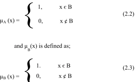
universe of discourse in sets A and B [1], respectively. The characteristic function, [10], μA(x) is defined as follows:
µA (x) =
{
and μ
B(x) is defined as;
µB (x) =
{
Using the above definitions, the following operations are defined;
2.1.1.1 UNION
The union between two sets, i.e., C = AỤB where Ụ is the union operator, represents all those elements in the universe which reside in either the set A or set B. The characteristic function μ
C is defined below:
µC (x) = max [µA (x), µB (x)] S.NO
.
Techno-Complexit
y
Practitione r Level
Revie w effort
Creatio n effort
Urgenc y
Actua l Faults
1 5 8 8 5 0 14
2 8 5 8 8 2 17
3 2 8 6 8 0 8
4 2 8 7 8 0 4
5 3 7 5 3 0 7
6 5 7 7 8 3 12
7 5 7 7 7 2 4
8 4 4 5 5 0 4
(2.2) 0, x ¢ B
1, x є B
(2.3) 0, x ¢ B
1, xєB
(2.4) Height in cm.
µ
c160
Fig. 3.1: Crisp set
The operator in above equation is referred to as the max-operator.
2.1.1.2 INTERSECTION
The intersection between two sets, i.e., C = A∩B where ∩ is the intersection operator, represents all those elements in the universe which reside in set A and set B simultaneously. The characteristic function μ
C is defined
below:
µC (x) = min [µA (x), µB (x)]
The operator in above equation is referred to as the min-operator
2.1.1.3 COMPLEMENT
The complement of a set A, denoted A, is defined as the collection of all elements in the universe which do not reside in the set A. The characteristic function is
A defined by
A
1
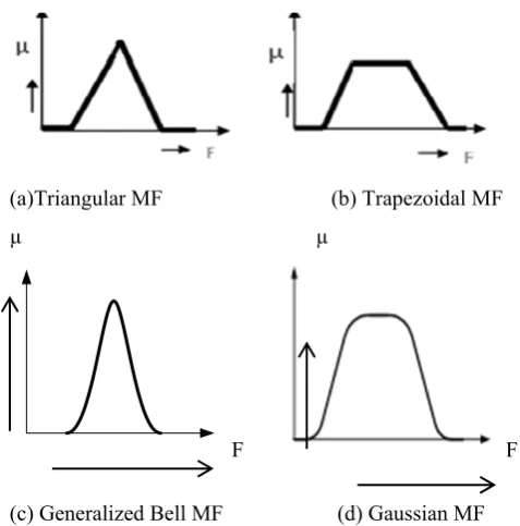
A 2.2 MEMBERSHIP FORMULATION:The membership functions for fuzzy sets can have many different shapes [27], depending on definition. All information contained in a fuzzy set is described by its membership function. Membership function allows assigning a level of membership for any variable “x” to the fuzzy set. Many types and shapes of membership functions can be used, Fig. 2.3 provides a description of the various shapes of membership functions;
(a)Triangular MF (b) Trapezoidal MF
µ µ
F
F
(c) Generalized Bell MF (d) Gaussian MF
Fig. 2.3: Membership functions with different shapes
One of the biggest differences between crisp and fuzzy sets is that the former always have unique MFs, whereas
every fuzzy set has an infinite number of MFs that may represent it. This is at once both a weakness and strength; uniqueness is sacrificed, but at the same time gives a gain in terms of flexibility, enabling fuzzy models to be "adjusted" for maximum utility in a given situation. e.g. consider the example in which each linguistic variable is fully characterized by a quintuple. The performance of the system is linguistically defined as Very small, Small, Medium, Large, Very large.
3 FUZZY INFERENCE ENGINE
The introduction of fuzzy set theory by Professor Lotfi A. Zadeh,[1], in 1965. Fuzzy logic provides a convenient way to represent Linguistic variables and subjective probability. The motivation and justification for fuzzy logic is that the linguistic characterizations are less specific than the numerical ones. Fuzzy logic targets handling real world problems. Most situations in the world require crisp actions; these actions (Decisions) are arrived at by processing fuzzy information (#Fig. 4.9). Fuzzy logic is used to provide means of inferring the fuzzy information to produce crisp actions, [12].
3.1 FUZZIFICATION
Fuzzification is the process of making the crisp quantity “fuzzy”. This allows addressing uncertainty in any parameter due to imprecision, ambiguity or vagueness. In artificial intelligence, the most common way to represent human knowledge is in terms of natural language i.e. linguistic variables. Depending upon the data and uncertainty, the input and the output parameters are fuzzified in terms of linguistic descriptors such as high, low, medium, and small to translate them into fuzzy variables. e.g. fuzzy boundaries for the parameter “age” can be formed by the linguistic expressions such as “young”, “middle aged”, and “old”. Thereafter, fuzzy sets for the input parameters and the required single output parameter are formulated based on the expert’s knowledge and experience in the particular domain.
There may be other influencing parameters, although there are no limits to the number of influencing parameters that can be used from a modeling perspective, [21]. For practical purposes however, two to four influencing parameters are sufficient to capture the major drivers of faults.
Linguistic descriptors such as High, Low, Medium, Small, Large, e.g., are assigned to a range of values for the output and for the input parameters. Since these descriptors form the basis for capturing expert input on the impact of input parameters on the number of faults, it is important to calibrate them to how they are commonly interpreted by the experts providing input. Referring to a variable as (2.5)
High, should evoke the same understanding among the experts.
Fuzzy sets for the inputs and the required single output are formulated based on the expert’s knowledge and experience in the particular domain (#Fig. 3.3) as per the development standards of the organization.
Membership values for the input parameters are calculated from the fuzzy sets drawn by the experts. These fuzzy sets form the basis for calculating membership values as per the specifications of the individual project.
3.2INFERENCE
Having specified the expected number of faults and its influencing parameters, the logical next step is to specify how the expected numbers of faults vary as a function of the influencing parameters, [13]. Experts provide fuzzy rules in the form of if … then statements that relate expected number of faults to various levels of influencing parameters based on their knowledge and experience. Fuzzy processor uses linguistic rules to determine what control action should occur in response to a given set of input values. Rule evaluation also referred as fuzzy inference, evaluates each rule with the inputs that were generated from the fuzzification process.
Syntax of rules;
IF antecedent 1 AND antecedent 2 AND THEN Consequent 1 AND ……...
e.g, considering the rules; “if A AND B then C.”
“if A’ AND B then C.”
For particular crisp input values, the degree of truth known as the membership value, for each antecedent is determined by using fuzzification transformation provided by the experts. All fuzzy statements in the antecedent are resolved to a degree of membership between 0 and 1.
Considering the membership values for the above rule as;
μ(x=A)= 0.5, μ(x=B)= 0.6 μ(x=A’)= 0.8, μ(x=B)= 0.6
The membership values are obtained from the fuzzy sets depending on specific values of the input parameters. The shape of a membership function affects the fuzzy operation in a subtle way.
Find rule strengths;
The fuzzy operators AND (Conjunction operator) or
OR (Disjunction operator) are applied to obtain the degree
of truth for the consequent of the rule, also known as the strength of entire rule, which is equal to the minimum of the antecedent degree of truth. This gives,
μ(x=A) ∩μ(x=B) = 0.5 ∩ 0.6= 0.5 = μ(x=C) μ(x=A’) ∩μ(x=B) = 0.8 ∩ 0.6 = 0.6 = μ(x=C)
Fuzzy outputs for each consequent label are determined which is equal to the maximum rule strengths or degree of support for each consequent label. For consequent C,
Fuzzy output = MAX (0.5, 0.6) = 0.6
The rules span all possible scenarios for combinations of all the levels of input parameters, thus completely mapping the input space of influencing parameters to the output space of expected number of faults. Degree of support is used for the entire rule to shape the output fuzzy set. The consequent of a fuzzy rule assigns an entire fuzzy set to the output. This fuzzy set is represented by a membership function that is chosen to indicate the qualities of the consequent. If the antecedent is only partially true, (i.e., is assigned a value less than 1), then the output fuzzy set is truncated according to the implication method. In general, one rule by itself doesn't do much good. Minimum two or more rules are needed that can play off one another. The output of each rule is a fuzzy set. The output fuzzy sets for each rule are then aggregated into a single output fuzzy set. Finally the resulting set is defuzzified, or resolved to a single number. The next section shows how the whole process works from beginning to end for a particular type of fuzzy inference system called a Mamdani type.
Mamdani-type inference expects the output membership functions to be fuzzy sets. After the aggregation process, there is a fuzzy set for each output variable that needs defuzzification. It's possible, and in many cases much more efficient, to use a single spike as the output membership functions rather than a distributed fuzzy set. This is sometimes known as a singleton output membership function, and it can be thought of as a pre-defuzzified fuzzy set. It enhances the efficiency of the defuzzification process because it greatly simplifies the computation required by the more general Mamdani method, which finds the centroid of a two-dimensional function. Rather than integrating across the two-dimensional function to find the centroid, the weighted average of a few data points is used. Sugeno-type systems support this type of model. In general, Sugeno-type systems can be used to model any inference system in which the output membership functions are either linear or constant.
3.3 COMPOSITION
inputs, [13]. The active conclusions are then combined into a logical sum for each membership function. A firing strength for each output membership function is computed. The fuzzy outputs for all rules are finally aggregated to one fuzzy set for various levels of consequent.
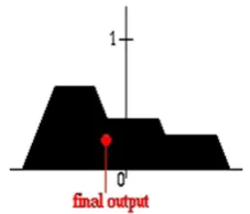
3.4 DEFUZZIFICATION
The logical sums are combined in the defuzzification process to produce the crisp output. To obtain a crisp decision from this fuzzy output, the fuzzy set, or the set of singletons have to be defuzzified. There are several heuristic methods (defuzzification methods), one of them is e.g. to take the center of gravity, [13], (#Fig. 3.10) of the fuzzy set, which is widely used for fuzzy sets. For the discrete case with singletons usually the mean of maxima method is used where the point with the maximum singleton is chosen.
Centre of gravity, calculates sum of the output and the corresponding membership function of the output fuzzy set and the weighted sum of the membership function. Formally, crisp value is the value located under the centre of gravity of the area, [13].
4 CONCLUSIONS
The actual faults and those obtained by implementing fuzzy expert system for predicting the expected number of faults before testing in 4 different projects are compiled in Table 5.1.
Table 5.1: Comparison between actual and predicted no. of faults using FL
The results above show the good and consistent fault predicting accuracy of the proposed model, with 90.2% correlation with the actual faults which is considered as
favorable models. The percentage error is also minimum for the proposed approach i.e. 18.72%. Moreover, from the results provided by fuzzy logic, the best and worst case performance for projects is effectively predicted by this method.
This analysis has presented a framework in which fuzzy expert rules might be used for detecting the number of faults in a program. This information is especially useful if predictions are to be made early in the life cycle of the software development.
The proposed method simplifies the difficult task of determining the fuzzy reliability of software using arithmetic operations of fuzzy sets much easier.
5 FUTURE SCOPES
The future scope is to collect samples of data from some more organizations, develop the proposed model and if possible validate them. In this proposed approach we can add some more parameters to improve the accuracy in prediction of software reliability. Implementation of model and Validate them.
REFERENCES
[1]. Michael R. Lyu,,”A Handbook of Software Reliability
Engineering”, New York, NY: McGrawHill / IEEE Computer Society Press. (1996)
[2]. Ann Marie Neufelder, “How to Measure the Impact of Specific Development.
[3]. Wood A, (1996) “Predicting Software Reliability”, IEEE Computers, 11:69-77.
[4]. K. Krishna Mohan, A. K. Verma, A. Srividya, (2009) “Selection of Fuzzy Logic Mechanism for Qualitative Software Reliability Prediction” ISSRE.
[5]. A. Bertolino, (2007), “Software Testing Research: Achievements, Challenges, Dreams,” Future of Software Engineering 2007, L. Briand and A. Wolf (eds.), IEEE-CS Press.
[6]. Agresti and Evanco, “Projecting Software Defects from Analyzing Ada Desings”, IEEE Transactions on Software Engineering, Vol. 18, No. 11, 1992.
[7]. J. McCall, W. Randell, J. Dunham, L. Lauterbach, “Software Reliability, Measurement, and Testing Software Reliability and Test Integration RL-TR-92-52”, Produced for Rome Laboratory, Rome, NY, 1992.
[8]. Wangbong Lee, Boo-Geum Jung, Jongmoon Baik, (2008), “Early reliability Prediction: An Approach to software Reliability Assessment in Open Software Adoption Stage”, IEEE Computer Society.
[9]. Smidts, et al, (1998), “Software Reliability Modeling: An Approach to Early Reliability Prediction”, IEEE Transactions on Reliability, Vol. 47, No. 3, pp 268-278
[10]. H.J. Zimmermann, Fuzzy set theory and its applications, 2nd ed., Allied Publisher Ltd, 1996.
[11]. Michael R. Lyu, (2007) “Software Reliability Engineering: A Roadmap”, IEEE Computers and Information Science, pp 153-170 [12]. K. Krishna Mohan, A. K. Verma, A. Srividya, (2009) “Selection of Fuzzy Logic Mechanism for Qualitative Software Reliability Prediction” ISSRE.
[13]. Riza C. Berkan, Sheldon L. Trubatch, “Fuzzy Systems Design Principles”, Building Fuzzy IF-THEN Rule Bases; IEEE PRESS, pp:70, 1997.
[14]. Military Handbook, “Electronic Design Handbook”, pp 35 to 9-37, 1998.
Projects Actual no. of Faults Predicted no. of Faults using FL
1 14 9.17
2 17 17.5
3 8 4.14
4 4 4.14
Correlation coefficient 0.902
Percentage error 18.72%