Cryptanalysis of the CHES 2009/2010
Random Delay Countermeasure
Fran¸cois Durvaux?, Mathieu Renauld??, Fran¸cois-Xavier Standaert? ? ?, Loic van Oldeneel tot Oldenzeel†, Nicolas Veyrat-Charvillon‡
Universit´e catholique de Louvain, UCL Crypto Group, B-1348 Louvain-la-Neuve, Belgium.
Abstract. Inserting random delays in cryptographic implementations is often used as a countermeasure against side-channel attacks. Most previ-ous works on the topic focus on improving the statistical distribution of these delays. For example, efficient random delay generation algorithms have been proposed at CHES 2009/2010. These solutions increase se-curity against attacks that solve the lack of synchronization between different leakage traces by integrating them. In this paper, we demon-strate that integration may not be the best tool to evaluate random delay insertions. For this purpose, we first describe different attacks exploiting pattern recognition techniques and Hidden Markov Models. Using these tools, we succeed in cryptanalyzing a (straightforward) implementation of the CHES 2009/2010 proposal in an Atmel microcontroller, with the same data complexity as an unprotected implementation of the AES Ri-jndael. In other words, we completely cancel the countermeasure in this case. Next, we show that our cryptanalysis tools are remarkably robust to attack improved variants of the countermeasure, e.g. with additional noise or irregular dummy operations. We also exhibit that the attacks remain applicable in a non-profiled adversarial scenario. Overall, these results suggest that the use of random delays may not be effective for pro-tecting small embedded devices against side-channel leakage. They also confirm the need of worst-case analysis in physical security evaluations.
1
Introduction
Protecting small embedded devices against side-channel attacks is a challeng-ing task. Followchalleng-ing the DPA book [17], maskchalleng-ing and hidchalleng-ing are two popular solutions to achieve this goal. Masking can be viewed as a type of data random-ization technique, in which the sensitive (key dependent) intermediate values in an implementation are split in different shares. One of its important outcomes is that, under certain physical assumptions (e.g. that the leakage of the different
?PhD student funded by the Walloon region MIPSs project. ??
PhD student funded by the Walloon region SCEPTIC project.
? ? ? Associate researcher of the Belgian fund for scientific research (FNRS-F.R.S.).
†
PhD student funded by the 7th framework European project TAMPRES.
‡
shares can be considered as independent), the security of a masked implemen-tation against side-channel attacks increases exponentially with the number of shares [3]. On the drawbacks side, masking usually implies significant perfor-mance overheads. In addition, the exponential security increase it theoretically guarantees is only effective when the amount of noise in the measurements (e.g. power or EM) is sufficient [25]. Hence, it is hardly useful as a standalone coun-termeasure for small cryptographic devices, and usually has to be combined with hiding. Roughly speaking, hiding aims at reducing the side-channel information by adding randomness to the leakage signal (rather than to the data producing it) and can take advantage of different methods. For example, the direct addi-tion of physical noise, or the design of dual-rail logic styles [27], are frequently considered options. Exploiting time randomization is a more flexible alternative, as it requires less (or no) modification of the underlying hardware.
Among the different time randomization techniques proposed in the litera-ture, e.g. [5, 14, 28], one can generally distinguish the software ones, e.g. based on Random Delay Interrupts (RDIs), from the hardware ones, e.g. based on in-creasing the clock jitter. Quite naturally, the more hardware-flavored is the coun-termeasure, the more signal-processing oriented are the solutions to overcome them [11, 19, 29]. In this paper, we pay a particular attention to the software-based solutions exploiting RDIs. In this setting, it is interesting to notice that most previous evaluations of the countermeasures impact (e.g. [16]) pre-process the leakage traces by integrating them. Somewhat biased by this evaluation technique, recent works such as the ones of Coron and Kizhvatov at CHES 2009/2010 [6, 7] mainly focused on how to improve the statistical distribution of the random delays, in order for their integration to produce the most noisy traces. However, looking at the source codes provided in these papers, that alter-nate actual cipher computations with dummy operations, a natural question is to ask whether techniques based on pattern recognition could not be used to di-rectly remove the delays. In other words, could it happen that, at least in certain contexts, this countermeasure can be strongly mitigated, or even reversed.
As previously observed in [10, 15], HMMs provide a very natural tool to deal with implementations in which some operations are randomized. We show experimen-tally that by adequately modeling a protected AES implementation as a HMM, we are able to produce traces that exactly correspond to the ones of an unpro-tected implementation, with very high probability. Eventually, it remains that the addition of RDIs prevents the use of averaging to improve the quality of an adversary’s measurements. Hence, we additionally evaluate the amount of noise that should be added to our measurements, in order for the countermeasure to become actually effective (i.e. to get closer to the security increases predicted in previous works using integration of the traces). It turns out the the application of HMMs is remarkably robust to noise addition. We conclude the paper by dis-cussing possible improvements of the countermeasure and their limitations, as well as a non-profiled variant of our HMM-based cryptanalysis.
We note that the authors in [6, 7] mention that it could be possible to detect random delays because of their regular pattern. They propose to hinder this by processing random dummy data during the delays, and acknowledge that this problem is not addressed in their papers. In the next sections, we show that identifying random delays in the power traces can be easy and that processing random dummy data is not sufficient to prevent attacks exploiting HMMs. Related work.In a recent and independent work, Strobel and Paar investigated the use of pattern matching for removing random delays in embedded software. Their proposal can be viewed as an alternative to our correlation-based tech-niques in Section 3. Namely, the work in [26] uses pattern matching in order to detect each random delayindependently and exploitshard informationmade of a string of Hamming weights obtained from power measurements. By contrast, our method in Section 4 models the complete assembly code of a protected AES implementation as a HMM (i.e. considers all the delays jointly) and exploits probabilistic information from the power traces. As a result, we obtain a better robustness to noise and hence, a more objective evaluation tool.
2
Background: the CHES 2009/2010 countermeasure
Overall, the addition of random delays in an implementation can be viewed as a trade-off between performance overheads (measured in code size and cycle count) and the variance added to the position of a target operation in side-channel measurement traces. In this section, we describe the countermeasure introduced at CHES 2009 (and improved at CHES 2010) by Coron and Kizhvatov, highlight their important characteristics and present our implementation.
security weaknesses. As a result, they proposed an improved solution, together with a new criterion to evaluate the security of RDI. In both cases, their imple-mentations ran on an 8-bit Atmel AVR platform, similar to the one we consider in this paper. In practice, the random delays were inserted at 10 places per AES round: once before AddRoundKey, once before each 32-bitSubBytesblock, once before each 32-bitMixColumnblock and once after the lastMixColumnblock.
Our implementation of the RDI countermeasure followed the same guidelines as in [6, 7] and was based on the AES-128 “furious” design, available as open source in [1]. Note that, as our goal is to identify and remove the delays from the traces, the actual distribution of their lengths has no incidence on our results. In other words, our focus is onhow the delays are inserted in the normal flow of the AES instructions, not on how much delay is inserted at each step1.
Algorithm 1Random delay insertion function
randomdelay:
(1) rcall randombyte 3 cycles
(2) tst RND 1 cycle
(3) breq zero 1 cycle (2 if true)
(4) nop 1 cycle
(5) nop 1 cycle
dummyloop:
(6) dec RND 1 cycle
(7) brne dummyloop 2 cycles (1 if false)
zero:
(8) ret 4 cycles
randombyte:
(9) ld RND, X+ 2 cycles
(10) ret 4 cycles
More precisely, the code we used in our evaluations is given as Algorithm 1. It is essentially the same as the one presented in [6], with the simplifiedrandombyte
function that only fetches some random numbers from a register2, and can be read as follows. Whenever a random delay needs to be inserted, therandomdelay
function is called. This function in turn calls (rcall) the randombytefunction that provides a value RND(that has to be carefully chosen in order to get good statistical distribution for the delay lengths). Depending on the valueRND, there
1
Similarly, the recommendation to add 3 dummy AES rounds with delays at the start and at the end of the AES computation, so that the target operations at the first and last rounds are separated from the synchronization points by at least 32 random delays, has little impact on our attacks exploiting HMMs.
2
are two cases: either RND = 0 and the function directly terminates by calling
zeroand returning (ret) to the normal flow of the AES instructions; orRND6= 0 and we enter the dummyloop. This loop simply consists in decrementing (dec)
RNDuntil it reaches 0, and the function terminates. The right part of Algorithm 1 indicates the number of cycles required by the different operations in our Atmel device. Hence, not considering the case where RND starts at 0, each delay is constituted of a header of 16 cycles, (RND−1) dummy loops of 3 cycles, a final dummy loop of 2 cycles, and at last aretinstruction of 4 cycles.
3
Pinpointing useful operation leakages
The previous section described the RDI countermeasure and the source code that we ran in an Atmel microcontroller. In this section, we show that the different operations in this target device produce significantly different leakages, that can be detected with simple tools based on correlation analysis. Beforehand, we briefly describe the setup we used to perform our experiments.
3.1 Measurement setup and preprocessing
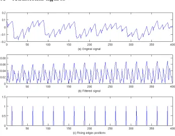
Our target device is an Atmel ATMega644P. Its power consumption has been measured at maximum clock frequency (i.e. 20Mhz3) and taken over a shunt resistor inserted in the supply circuit of the microcontroller. Sampled data was acquired with a Tektronix TDS7k oscilloscope. In order to facilitate our attack, we applied a simple preprocessing step. Namely, we first split the traces into con-secutive clock cycles, using the Fast Fourier Transform to recover the rising edges of the clock signal. This was achieved by filtering the frequency spectrum around the clock frequency and its harmonics, then applying the inverse transform on the filtered signal. This preprocessing provides a sequence of peaks indicating where the rising edges of the clock signal are. Following, we were able to work on a sequence of clock cycles instead of raw side-channel traces. It both reduced the difficulty of the attack and its computational cost. The steps of this filtering are illustrated in Appendix, Figure 7: the original trace (a) is first filtered in the spectral domain around the harmonics of the clock signal (b). By taking the local maxima, we get a decomposition of the trace into clock cycles.
3.2 Correlation based attacks
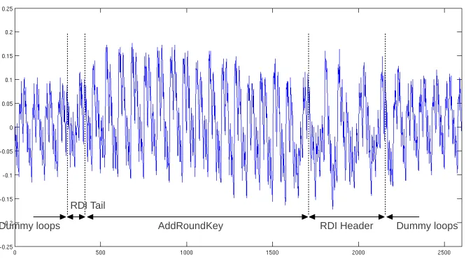
Let us first have a look at the power traces of an AES implementation protected with the RDI countermeasure. As illustrated by Figure 1, a simple visual inspec-tion allows determining the different parts of the code. In other words, there are significant operation leakages that can be detected with Simple Power Analysis. Two main approaches can be considered for this purpose.
3 This work frequency result in slightly more noisy traces than if running at lower
AddRoundKey RDI Header Dummy loops
RDI Tail
Dummy loops
Fig. 1.AddRoundKey operation protected with the random delay countermeasure.
On the one hand, one can target the dummy operations, i.e. find the clock cycles during which thedummyloopis executed. As emphasized in Figure 2, ran-dom delays present a very distinctive outlook, since they contain short repetitive patterns, each loop lasting only three clock cycles. As a result, given that one can extract the pattern of this loop (including its header or tail), it is possible to match this pattern to clock cycles in the side-channel traces, by computing the cross-correlation between them. Eventually, the adversary can filter the traces by removing any cycle which is highly correlated with the delay pattern and attack the filtered traces, e.g. with Correlation Power Analysis (CPA) [2].
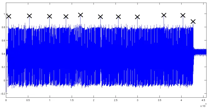
On the other hand, the adversary can also target the actual AES operations, instead of the delays. Indeed, while the inserted delays are of variable length and their shape can be changed, the AES operations are fixed andhaveto be executed by the program. It turns out that this detection is specially easy when large sequences of operations are executed without dummy operations. For example, AddRoundKey is rather distinctive in the proposal of [6, 7], as it consists in sixteen three-cycle loops surrounded by RDI delays. Hence, if the part of the power trace that corresponds to this sequence of operations can be extracted in a preliminary profiling, it can be compared with other side-channel traces using cross-correlation, just as for the detection of dummy operations. An exemplary result of this detection technique is given in Figure 3. It highlights that significant information on the executed operations is available in our measurements, and that integrating traces is not the best approach for analyzing RDIs.
Fig. 2.Zoom on the RDI header and dummy operations.
1. On improving the countermeasure. In the first place, the previous figures ad-mittedly target the direct application of the CHES 2009/2010 countermeasures. However, while the choice of dummy operations to execute has little or no im-pact on “integrating” attacks, it is critical when playing with pattern matching as we undertake in this paper. In particular, two simple improvements could be implemented. First, one could use AES operations in the dummy cycles. Sec-ond, the hardware interrupts of the Atmel microcontroller could be exploited, in order for the RDIs to occur at less predictable places (e.g. the guarantee that AddRoundKeyis executed as a single block would vanish in this case).
2. On the heuristic nature of the correlation-based approach. Second, it is worth emphasizing that the previous exploitation of cross-correlation is essentially heuristic. While it is intuitively useful to put forward a risk of attacks, it is also limited and hardly generic. In particular, if the aforementioned improvements were implemented, cross-correlation based attacks would become ineffective.
3. On the meaning of Kerckhoffs’ principles in implementation attacks. Even-tually, the analysis of RDIs raises the question of what the adversary exactly knows about his target implementation. In general, cryptographers like to con-sider that most possible information (e.g. about the algorithms) is public and that security only relies on the secrecy of a key. Straightforwardly translating this principle in the physical world would imply that source codes are given to the adversary, a condition that may not always be found in the field though. Such a question directly relates to the question of profiled vs. non-profiled attacks as well. For example, in the previous discussion of correlation-based attacks, is it realistic that the adversary can build an approximate pattern for the dummy operations or AES operations? In the following, we will essentially investigate the case where the answer is yes and justify this choice with three main reasons. Besides, we also provide a non-profiled solution to our problem in Section 4.6.
1. In practice, the gap between profiled and non-profiled attacks, and the lack of knowledge about the underlying hardware and implementation, can usually be overcome in the long term. Examples of solutions to reduce this gap in-clude the use of non-profiled stochastic models [9, 21], or techniques inspired from side-channel attack reverse engineering [8, 12, 20].
2. In general in cryptography, a security evaluation has to look for worst cases, and this also applies to implementation attacks [24]. Hence, regardless the practical relevance of certain adversarial scenarios, it is essential to consider them, in order to have a fair understanding of the actual security level pro-vided by cryptographic implementations. Practical security can of course be higher than what is lower-bounded by worst-case attacks.
and source code (including the exact time instants when the shares are ma-nipulated), the analysis of Chari et al. [3] still holds and the data complexity of an attack against this implementation can still be high enough4.
4
Hidden Markov model cryptanalysis
Having justified the need of optimal evaluation tools, this section investigates a new cryptanalysis of RDIs based on HMMs. We argue that it constitutes an interesting generic tool to capture our problem. In particular, and contrary to the correlation-based techniques, it can easily deal with any type of dummy op-erations and interrupt processes. As mentioned in introduction, this approach follows previous works in the field of reverse engineering and cryptanalysis of randomized implementations, where similar principles have been used [10, 15]. In particular, the work of Karlov and Wagner is very similar to ours as it exploits HMMs to break the randomized exponentiation algorithms. To a certain extent, removing random delays in side-channel traces can also be seen as a simplified reverse engineering problem. That is, Eisenbarth et al. intend to build a disas-sembler, in order to extract an exact sequence of unknown instructions being executed by a device. We follow the same goal in the case where the instructions are known but the number of dummy loops that are executed for each delay is unknown. In the following, we first explain how to translate the RDI detection as a HMM problem. Next, we describe how to actually remove the delays from side-channel leakage traces and present results of experimental attacks against our randomized implementation. Eventually, we discuss possible improvements of the countermeasure as well as a non-profiled variant of the attack.
4.1 Building the HMM
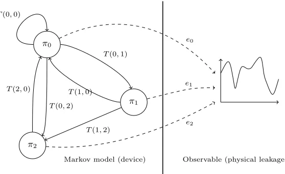
A Markov model is a (memoryless) system with a finite number of states, for which the probabilities of transition to the next state only depend on the current state. It is thus constituted of a set of states πi’s and a transition probability matrix T. T(i, j) is the (a priori) probability that the next state is πj if the current state isπi. If we denote withstthe current state of the system at time t,T(i, j) = Pr(st+1 =πj|st =πi). In the case of a Hidden Markov model, the sequence s= (s0, s1, ..., sn) of the states occupied by the system is not known. However, the adversary has access to (at least) one observable that gives partial information about this sequence. Namely, at each time stept, a random vector ltis observed by the adversary. In addition to the transition probability matrix, the HMM is then characterized by the emission probability functions associated to each stateπi, namely:ei(lt) = Pr(lt|st=πi) (see Figure 4).
4
π0
π1
π2
T(0,0)
T(0,1)
T(1,0)
T(1,2) T(0,2)
T(2,0)
e0
e1
e2
Markov model (device) Observable (physical leakage)
Fig. 4.Hidden Markov Model. The Markov model represents the device executing a sequence of instructions. The observable is the physical leakage.
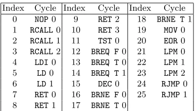
In the case of our protected AES implementation, the Markov model de-scribes the encryption process, with each state πi associated to an instruction (e.g. NOP, RET, ...). Some instructions take only one clock cycle, but others re-quire several clock cycles to be completed. As each state should correspond to the same number of clock cycles, longer instructions are split in different states, e.g.RCALLtaking 3 cycles is split in three states associated toRCALL0,RCALL1 and RCALL 2. We call instruction cycle the (part of an) instruction associated with a state πi. The list of all the 26 instruction cycles5 appearing in the code of the protected AES can be found in Table 1. Note that the same instruction cycle can be used at multiple places in the AES code, corresponding to different running states, e.g.π0↔MOV0,π1↔EOR0,π2↔MOV0, . . .
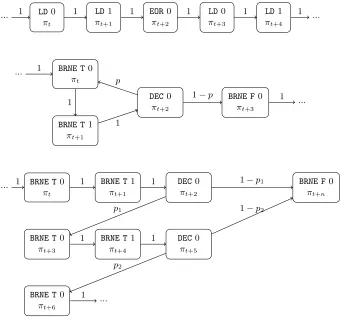
More precisely, the protected AES code can be divided in two types of instruc-tion sequences: the deterministic instrucinstruc-tion sequences and the dummy loops. In the deterministic sequences, the instruction cycle associated to a state is fully determined by its position in the sequence. In order to model these determinis-tic sequences, we can simply use one different state per successive cycle in the sequence, with deterministic transition probabilities:T(i, i+ 1) = 1 (see the top of Figure 5). By contrast, the non-deterministic dummy loops are constituted of a branching (BRNE) and a decrement (DEC) instruction. This translates into 4 instruction cycles: BRNE T 0, BRNE T 1 andDEC 0 in the loop (i.e. while the counter is decremented), and eventuallyBRNE F0 to end the loop. There are two main ways to encode these loops in a Markov model. The simplest one consists in using 4 states, as presented in the middle part of Figure 5. The transition
5
Index Cycle Index Cycle Index Cycle
0 NOP0 9 RET2 18 BRNE T1
1 RCALL0 10 RET3 19 MOV0
2 RCALL1 11 TST0 20 EOR0
3 RCALL2 12 BREQ F0 21 LPM0
4 LDI0 13 BREQ T0 22 LPM1
5 LD0 14 BREQ T1 23 LPM2
6 LD1 15 DEC0 24 RJMP0
7 RET0 16 BRNE F0 25 RJMP1
8 RET1 17 BRNE T0
Table 1.List of instruction cycles occurring in the protected AES implementation.
probabilities at the output of the DECstate are pto restart another loop, and 1−pto exit the loop. This representation uses a fixed probabilityp, that cannot be changed based on the number of loops previously executed. It is thus not possible to render the details of the probability distribution of the delay lengths. Another way is to “unfold” the dummy loops by using 255×3 + 1 states, as in the lower part of Figure 5 (255 being the maximum number of dummy loops in one delay). It is then possible to fine tune the probabilities p1, p2, ..., in order to match the probability distribution of the delay lengths as closely as possible. In terms of performances, the second representation is more precise and al-lows capturing the AES implementation more accurately, potentially leading to a better robustness against noisy measurements. However, its larger number of states also implies a more complex resolution phase (in time and memory). As experimental results showed that the compact representation was sufficient to obtain successful attacks with low data complexity, we focus on this one in the rest of the paper. Eventually, our Markov model for the protected AES imple-mentation has approximately 6000 states, each of them associated to one of the 26 different instruction cycles from Table 1. The corresponding transition matrix T is very sparse, as the sequence of instructions is deterministic most of the time (in which caseT(i, i+ 1) = 1 is the only non-zero value of theith line).
4.2 Building the templates
Once the Markov model corresponding to the protected AES is determined, we still have to estimate the emission probability functions ei(lt) = Pr(lt|st =πi) corresponding to each stateπi. We make two assumptions for this purpose:
1. The power trace lcan be cut cycle in cycles:l= (l0,l1, ...). This is possible using the FFT-based technique of Section 3.1. We denote with trace cycle each partliof the power trace corresponding to one clock cycle. Trace cycles are measured vectors of 25 values (obtained with the setup of Section 3.1). 2. The emission at time t, denoted as lt, only depends on the type of the
... LD0
πt
LD1
πt+1
EOR0
πt+2
LD0
πt+3
LD1
πt+4
...
1 1 1 1 1 1
... BRNE T0
πt
BRNE T1
πt+1
DEC0
πt+2
BRNE F0
πt+3
... 1
1
1
p
1−p 1
... BRNE T0
πt
BRNE T1
πt+1
DEC0
πt+2
BRNE T0
πt+3
BRNE T1
πt+4
DEC0
πt+5
BRNE T0
πt+6
...
BRNE F0
πt+n
1 1 1
p1
1−p1
1 1
p2
1−p2
1
Estimating the emission probability functions is equivalent to building a template for each stateπi. But contrarily to standard side-channel template attacks, where templates are built from a single instruction in order to distinguish the data being processed (e.g. [4]), we build templates for the different instruction cycles in order to tell them apart. That is, as our Makov Model contains 6000 states, we could build up to 6000 templates. But thanks to our second assumption, the same template can be used for every stateπi associated to the same instruction cycle from Table 1. Hence only 26 templates are required for the 6000 different states. Next, the emission probability functions are directly determined by these templates: for an instruction cyclei, we have the functionei(lt) =N(lt|µˆi,Σˆi). For each template, the mean vector ˆµi and correlation matrix ˆΣi are estimated from a set of trace cycles lt corresponding to the same instruction cyclei.
In order to build these 26 templates, we thus need to find sets of trace cycles ltcorresponding to each possible instruction cycle. However, due to the unknown lengths of the delays in a protected implementation, it is impossible to directly match trace cycles to their corresponding instruction cycles. As a result, we used a profiling phase for this purpose. That is, we built the templates from a train-ing device for which the length of the delays was fixed. In addition, we used this profiling phase in order to efficiently reduce the dimensionality of our traces cy-cles, using the Principal Component Analysis (PCA) technique described in [23]. PCA consists in linearly projecting the data (i.e. the trace cycles) on a lower dimensional subspace, in such a way that the variance between the different in-struction cycles is maximized. In practice, we kept 3 dimensions per template, which appeared to be a good compromise between the amount of variability we retain and the complexity of the parameters we need to evaluate.
4.3 Removing the delays
stept≥1 and each statei, the indexj of the most probable state sequence of lengtht−1 that can lead to statei:I(i, t−1) = argmaxj(V(j, t−1)·T(j, i)). Once the full sequence of observation is processed, the algorithm selects the most prob-able ending state, and then backtracks to the first observation using the matrix I to select at each step the previous state in the most probable sequence.
Algorithm 2Viterbi algorithm
input: a HMM characterized by a set of Ns states πi, initial probabilities pi, a transition probability matrixT and emission probability functionsei.
input:a sequence ofNo observationsl= (l0,l1, ...).
output:the most probable sequence of states corresponding to the observations. DefineV a new matrix inRNs×No.
DefineIa new matrix in NNs×(No−1).
//Initial probabilities. fori= 0 toi=Ns−1do
V(i,0)←pi·ei(l0)
end for
//Computing the probabilities. fort= 1 tot=No−1do
fori= 0 toi=Ns−1do
V(i, t)←ei(lt)·maxj(V(j, t−1)·T(j, i))
I(i, t−1)←argmaxj(V(j, t−1)·T(j, i)) end for
end for
//Backtracking to find the most probable path. Definesa new vector of sizeNo.
s(No−1)←argmaxj(V(j, No)) fort=no−2 tot= 0do
s(t)←I(s(t+ 1), t) end for
return s
4.4 Results of the HMM method and impact of the noise
from a set of 100 independent experiments. In fact, the slight difference between protected and unprotected implementations can be explained by the postpro-cessing of the traces after removing the RDIs, because of slight imperfections of the cycles cut. Otherwise, the actual removing of the delays was close to 100% successful. As a result, both implementations can be broken after approximately 100 measurements. For comparison, the integration attack on the protected im-plementation in [6] requires approximately 45 000 power traces to succeed. We conclude that (1) the HMM method is much more efficient than the integration method to attack the RDI countermeasure, and (2) with the actual noise level of an Atmel 8-bit microcontroller, the RDI countermeasure is completely reversible.
100 101 102 103 104
0 0.2 0.4 0.6 0.8 1
data complexity (number of traces)
CP
A
success
rate
σ∗= 0
σ∗= 0.025
σ∗= 0.1
σ∗= 0.2
Fig. 6.Success rate of a CPA attack in different scenarios. The plain lines correspond to the attack on an unprotected implementation, the dashed lines correspond to the attack on a protected implementation with RDI removed by the HMM method.σ∗ is the standard deviation of the simulated Gaussian noise added to the traces,σ∗ = 0 corresponds to the real noise level. The delays are efficiently removed up toσ∗= 0.1
in this case). However, whenσ∗goes beyond 0.1, it becomes increasingly harder to correctly detect the delay lengths. And byσ∗= 0.2, the HMM method does not correctly identify the delay lengths anymore. In conclusion, the RDI counter-measure has an impact on security only when the noise level is high enough for a successful CPA attack against the corresponding unprotected implementation to require more than 10 000 traces. This unfortunately goes against the goal of using RDIs to emulate noise for small embedded (e.g. 8-bit) devices.
σ∗= 0σ∗= 0.025 σ∗= 0.1 σ∗= 0.2 SNR 0.2 0.014 1.34×10⁻³ 2.44×10⁻⁴
Table 2.SNR of the unprotected implementation with additive simulated noiseσ∗.
4.5 RDI improvements
The HMM method is very efficient against the RDI countermeasure presented in [6, 7], in part due to the very regular pattern of the delays. It is thus natural to think about possible methods to make the delays and the actual AES com-putations harder to tell apart. In the following of this section, we discuss some proposals that could be used to achieve this goal, and their limitations.
One straightforward idea is to use delays with no regular pattern, e.g. delays made of random instructions. However, implementing the RDI countermeasure in this case will still require (1) a specific deterministic header containing the in-structions needed to determine the delay length, and (2) a loop ensuring that the delay stops after a given counter has reached 0. Using the hardware interrupts feature of the Atmel microcontrollers would not help in this respect, as dealing with these interrupts also gives rise to (4 or 5) very distinguishable cycles. In addition, even if the delays had a perfectly random pattern, the AES operations would still have to be processed, and could be identified with the Viterbi algo-rithm. For illustration, we ran experiments with hypothetical simulated traces, where the delays only consisted in random instructions instead of dummy loops. That is, these simulated traces do not contain any identifiable header or tail. We recall that this context is unrealistic as such headers and tails are needed to implement the countermeasure and generally provide useful information to the adversary. But even this minimum leakage could be efficiently exploited. Namely, while the Viterbi algorithm was not always able to accurately predict the instructions processed during the delays, it was still able to correctly identify the position of the AES instruction sequences. Hence, as illustrated in Appendix, Figure 8, such an idea is not sufficient to prevent successful attacks. Yet, one can notice that it reduces the noise robustness of the HMM cryptanalysis.
real data and the rest on dummy data. This way, the HMM method provides no information on where are the delays, as the delays are totally indistinguishable from the AES computations. Unfortunately, this countermeasure provides little security at high cost: instead of attacking one time sample, the adversary will simply have to integrate overn. Eventually, we conjecture that solutions to im-prove the time randomization of cryptographic implementations should combine RDIs with other ideas, e.g. shuffling [13] or clock jitter. We leave the analysis of these combined scenarios as an interesting scope for further research.
4.6 A non-profiled version of the HMM method
The previous sections assumed the adversary can perform a profiling phase on a test device. Although justified in a security evaluation context, this assumption may not always be verified in practice. In the following, we finally show that even in a non-profiled context, it is possible to perform efficient HMM-based attacks against an RDI-protected implementation, by exploiting clever “on-the-fly” characterization of the the target device, with a single leakage trace.
5
Conclusions
The investigations in this paper confirm the discussion in [22] that protections against side-channel attacks based on time randomizations are challenging to evaluate, as they may easily provide a false sense of security, whenever they are reversible with the appropriate signal processing / statistical / modeling tools. The case of RDIs is a good illustration of this concern: we show that their im-plementation in a low-cost microcontroller can be completely reversed and that making them effective is a non-trivial task (e.g. software-based improvements are unlikely to be sufficient). Hence, the study of other time randomization tech-niques such as shuffling [13], or the combination of RDIs with other countermea-sures against side-channel attacks, are interesting research problems. Besides, RDIs are also considered as a solution to prevent fault attacks. In this setting, it is an interesting question to determine whether the HMM-based cryptanalysis could be applied “on-the-fly” during a fault attack, in order to help adversaries to insert faults in the sensitive computations of randomized implementations.
References
1. http://point-at-infinity.org/avraes/.
2. Eric Brier, Christophe Clavier, and Francis Olivier. Correlation power analysis with a leakage model. In Marc Joye and Jean-Jacques Quisquater, editors,CHES, volume 3156 ofLecture Notes in Computer Science, pages 16–29. Springer, 2004. 3. Suresh Chari, Charanjit S. Jutla, Josyula R. Rao, and Pankaj Rohatgi. Towards
sound approaches to counteract power-analysis attacks. In Michael J. Wiener, editor,CRYPTO, volume 1666 ofLecture Notes in Computer Science, pages 398– 412. Springer, 1999.
4. Suresh Chari, Josyula R. Rao, and Pankaj Rohatgi. Template attacks. In Burton S. Kaliski Jr., C¸ etin Kaya Ko¸c, and Christof Paar, editors,CHES, volume 2523 of Lecture Notes in Computer Science, pages 13–28. Springer, 2002.
5. Christophe Clavier, Jean-S´ebastien Coron, and Nora Dabbous. Differential power analysis in the presence of hardware countermeasures. In C¸ etin Kaya Ko¸c and Christof Paar, editors,CHES, volume 1965 ofLecture Notes in Computer Science, pages 252–263. Springer, 2000.
6. Jean-S´ebastien Coron and Ilya Kizhvatov. An efficient method for random de-lay generation in embedded software. In Christophe Clavier and Kris Gaj, edi-tors, CHES, volume 5747 of Lecture Notes in Computer Science, pages 156–170. Springer, 2009.
7. Jean-S´ebastien Coron and Ilya Kizhvatov. Analysis and improvement of the ran-dom delay countermeasure of ches 2009. In Stefan Mangard and Fran¸cois-Xavier Standaert, editors, CHES, volume 6225 of Lecture Notes in Computer Science, pages 95–109. Springer, 2010.
8. R´emy Daudigny, Herv´e Ledig, Fr´ed´eric Muller, and Fr´ed´eric Valette. Scare of the des. In John Ioannidis, Angelos D. Keromytis, and Moti Yung, editors, ACNS, volume 3531 ofLecture Notes in Computer Science, pages 393–406, 2005.
10. Thomas Eisenbarth, Christof Paar, and Bj¨orn Weghenkel. Building a side channel based disassembler. Transactions on Computational Science, 10:78–99, 2010. 11. Sylvain Guilley, Karim Khalfallah, Victor Lomn´e, and Jean-Luc Danger. Formal
framework for the evaluation of waveform resynchronization algorithms. In Clau-dio Agostino Ardagna and Jianying Zhou, editors,WISTP, volume 6633 ofLecture Notes in Computer Science, pages 100–115. Springer, 2011.
12. Sylvain Guilley, Laurent Sauvage, Julien Micolod, Denis R´eal, and Fr´ed´eric Valette. Defeating any secret cryptography with scare attacks. In Michel Abdalla and Paulo S. L. M. Barreto, editors,LATINCRYPT, volume 6212 ofLecture Notes in Computer Science, pages 273–293. Springer, 2010.
13. Christoph Herbst, Elisabeth Oswald, and Stefan Mangard. An aes smart card implementation resistant to power analysis attacks. In Jianying Zhou, Moti Yung, and Feng Bao, editors,ACNS, volume 3989 ofLecture Notes in Computer Science, pages 239–252, 2006.
14. James Irwin, Dan Page, and Nigel P. Smart. Instruction stream mutation for non-deterministic processors. InASAP, pages 286–295. IEEE Computer Society, 2002.
15. Chris Karlof and David Wagner. Hidden markov model cryptoanalysis. In Walter et al. [30], pages 17–34.
16. Stefan Mangard. Hardware countermeasures against dpa ? a statistical analysis of their effectiveness. In Tatsuaki Okamoto, editor,CT-RSA, volume 2964 ofLecture Notes in Computer Science, pages 222–235. Springer, 2004.
17. Stefan Mangard, Elisabeth Oswald, and Thomas Popp. Power analysis attacks -revealing the secrets of smart cards. Springer, 2007.
18. Stefan Mangard, Elisabeth Oswald, and Fran¸cois-Xavier Standaert. One for all - all for one: Unifying standard dpa attacks. IET Information Security, 5 (2), 2011:100–110.
19. Sei Nagashima, Naofumi Homma, Yuichi Imai, Takafumi Aoki, and Akashi Satoh. Dpa using phase-based waveform matching against random-delay countermeasure. InISCAS, pages 1807–1810. IEEE, 2007.
20. Denis R´eal, Vivien Dubois, Anne-Marie Guilloux, Fr´ed´eric Valette, and M’hamed Drissi. Scare of an unknown hardware feistel implementation. In Gilles Grimaud and Fran¸cois-Xavier Standaert, editors,CARDIS, volume 5189 ofLecture Notes in Computer Science, pages 218–227. Springer, 2008.
21. Werner Schindler, Kerstin Lemke, and Christof Paar. A stochastic model for dif-ferential side channel cryptanalysis. In Josyula R. Rao and Berk Sunar, editors, CHES, volume 3659 ofLecture Notes in Computer Science, pages 30–46. Springer, 2005.
22. Fran¸cois-Xavier Standaert. Some hints on the evaluation metrics and tools for side-channel attacks. Non-Invasive Attacks Testing Workshop, Nara, Japan, September 2011, http://perso.uclouvain.be/fstandae/PUBLIS/107 slides.pdf.
23. Fran¸cois-Xavier Standaert and C´edric Archambeau. Using subspace-based tem-plate attacks to compare and combine power and electromagnetic information leakages. In Elisabeth Oswald and Pankaj Rohatgi, editors, CHES, volume 5154 ofLecture Notes in Computer Science, pages 411–425. Springer, 2008.
25. Fran¸cois-Xavier Standaert, Nicolas Veyrat-Charvillon, Elisabeth Oswald, Benedikt Gierlichs, Marcel Medwed, Markus Kasper, and Stefan Mangard. The world is not enough: Another look on second-order dpa. In Masayuki Abe, editor,ASIACRYPT, volume 6477 ofLecture Notes in Computer Science, pages 112–129. Springer, 2010. 26. Daehyun Strobel and Christof Paar. An efficient method for eliminating random delays in power traces of embedded software. In Howon Kim, editor,ICISC, volume xxxx ofLecture Notes in Computer Science, pages yyy–zzz. Springer, 2011. 27. Kris Tiri and Ingrid Verbauwhede. Securing encryption algorithms against dpa at
the logic level: Next generation smart card technology. In Walter et al. [30], pages 125–136.
28. Michael Tunstall and Olivier Benoˆıt. Efficient use of random delays in embed-ded software. In Damien Sauveron, Constantinos Markantonakis, Angelos Bilas, and Jean-Jacques Quisquater, editors, WISTP, volume 4462 of Lecture Notes in Computer Science, pages 27–38. Springer, 2007.
29. Jasper G. J. van Woudenberg, Marc F. Witteman, and Bram Bakker. Improving differential power analysis by elastic alignment. In Aggelos Kiayias, editor, CT-RSA, volume 6558 ofLecture Notes in Computer Science, pages 104–119. Springer, 2011.
A
Additional figures
Fig. 7.CPU’s clock rising edges detection on power traces.
100 101 102 103
0 0.2 0.4 0.6 0.8 1
data complexity (number of traces)
CP
A
success
rate
σ∗= 0
σ∗= 0.025