Numerical solution of variational problems via parametric quintic spline method

ISSN: 2251-8436 print/2322-1666 online

NUMERICAL SOLUTION OF VARIATIONAL PROBLEMS VIA PARAMETRIC QUINTIC SPLINE

METHOD

MOHAMMAD ZAREBNIA AND ZAHRA SARVARI

Abstract. In this paper, the parametric quintic spline method is

used for finding the solution of variational problems associated in en-gineering and physics. The present approximation reduce the prob-lems to an explicit system of algebraic equations. Some numerical examples are also given to illustrate the accuracy and applicability of the presented method.

Key Words: Calculus of variation, Parametric quintic spline, Boundary value problem.

2010 Mathematics Subject Classification:Primary: 34L99; Secondary: 65D05, 65D07.

1. Introduction

The need for an optimum function, rather than an optimal point, arises in numerous problems from a wide range of fields in engineering and physics, which include optimal control, transport phenomena, optics, elas-ticity, vibrations, statics and dynamics of solid bodies and navigation [1]. The calculus of variations and its extensions are devoted to finding the optimum function that gives the best value of the economic model and satisfies the constraints of a system. . In computer vision the calculus of variations has been applied to such problems as estimating optical flow [2] and shape from shading [3]. Several numerical methods for approxi-mating the solution of problems in the calculus of variations are known. Galerkin method is used for solving variational problems in [4]. The Ritz method [5], usually based on the subspaces of kinematically admissible

Received: 6 January 2013, Accepted: 18 April 2014. Communicated by A. Borhanifar; ∗Address correspondence to Mohammad Zarebnia; E-mail: [email protected]

c

2014 University of Mohaghegh Ardabili. 40

complete functions, is the most commonly used approach in direct meth-ods of solving variational problems. Chen and Hsiao [6] introduced the Walsh series method to variational problems. Due to the nature of the Walsh functions, the solution obtained was piecewise constant. Some orthogonal polynomials are applied on variational problems to find the continuous solutions for these problems [7]-[9]. A simple algorithm for solving variational problems via Bernstein orthonormal polynomials of degree six is proposed by Dixit et al. [10]. Razzaghi et al. [11] applied a direct method for solving variational problems using Legendre wavelets. Chebyshev finite difference method has been employed for solving some problems in calculus of variations in [12].

Spline functions are special functions in the space of which approximate solutions of ordinary differential equations. In other words spline function is a piecewise polynomial satisfying certain conditions of continuity of the function and its derivatives. The applications of spline as approximating, interpolating and curve fitting functions have been very successful[13]-[16]. In [17], a non-polynomial spline technique has been developed for the numerical solutions of a system of fourth order boundary value problems associated with obstacle, unilateral and contact problems. Polynomial and non-polynomial spline functions based methods have been presented to find approximate solutions to second order boundary value problems [18]. Khan [19] used parametric cubic spline function to develop a numer-ical method, which is fourth order for a specific choice of the parameter. Parametric spline approach to the solution of a system of second-order boundary-value problems has been proposed by Khan et al. [20]. Rashi-dinia et al. [21]-[22] used non-polynomial quintic spline method for the solution of a system of obstacle problems. Also Sinc-Galerkin method has been used for the solution of problems in calculus of variations in [23]. The main purpose of the present paper is to use parametric quintic spline method for numerical solution of boundary value problems which arise from problems of calculus of variations. The method consists of reducing the problem to a set of algebraic equations.

The outline of the paper is as follows. First, in Section 2 we introduce the problems in calculus of variations and explain their relations with boundary value problems. Section 3 outlines parametric quintic spline and basic equations that are necessary for the formulation of the discrete

system. Also in this section, we report our numerical results and demon-strate the efficiency and accuracy of the proposed numerical scheme by considering two numerical examples.

2. Statement of the problem

The genaral form of a variational problem is finding extremum of the functional

(2.1)

J[u1(t), u2(t), . . . , un(t)] =

Z b

a

G t, u1(t), u2(t), . . . , un(t), u01(t), u02(t), . . . , u0n(t)

dt.

To find the extreme value ofJ, the boundary conditions of the admis-sible curves are known in the following form:

ui(a) =γi, i= 1,2, . . . , n,

(2.2)

ui(b) =δi, i= 1,2, . . . , n.

(2.3)

The necessary condition for ui(t), i = 1,2, . . . , n to extremize

J[u1(t), u2(t), . . . , un(t)] is to satisfy the Euler-Lagrange equations that is

obtained by applying the well known procedure in the calculus of variation [5],

(2.4) ∂G

∂ui − d dt

∂G

∂u0_i

= 0, i= 1,2, . . . , n,

subject to the boundary conditions given by Eqs. (2.2)-(2.3).

In this paper, we consider the spacial forms of the variational problem (2.1) as

(2.5) J[u(t)] =

Z b

a

G t, u(t), u0(t)dt,

with boundary conditions

(2.6) u(a) =γ, u(b) =δ,

(2.7) J[u1(t), u2(t)] =

Z b

a

G t, u1(t), u2(t), u01(t), u02(t)

dt,

subject to boundary conditions

u1(a) =γ1, u1(b) =δ1,

(2.8)

u2(a) =γ2, u1(b) =δ2.

(2.9)

Thus, for solving the variational problems (2.5), by using Euler La-grange Eq. (2.4) we consider the second-order differential equation

(2.10) ∂G

∂u − d dt

∂G

∂u0

= 0,

with the boundary condition (2.6). And also, for solving the varia-tional problems (2.7), we find the solution of the system of second-order differential equations

(2.11) ∂G

∂ui

− d

dt

∂G

∂u0_i

= 0, i= 1,2,

with the boundary conditions (2.8)-(2.9). Therefore, by applying para-metric quintic spline method for the Euler-Lagrange equations (2.10) and (2.11) we can obtain an approximate solution to the variational problems (2.5) and (2.7).

3. Parametric quintic spline method

Consider the partition ∆ of [a, b] ⊂ R. Let Sk(∆) denote the set of

piecewise polynomials of degreekon subintervalIi= [ti−1, ti] of partition

∆. In this work, we consider parametric quintic spline method for finding approximate solution of variational problems.

Consider the grid pointsti on the interval [a, b] as follows: a=t0 < t1< t2< . . . , tn−1 < tn=b,

(3.1)

ti =t0+ih, i= 0,1,2, . . . , n,

(3.2)

h= b−a

n ,

(3.3)

where n is a positive integer. Let S∆(t, τ)(t) be quintic spline function

S∆(t, τ) depends on a parameter τ >0 that is called a parametric spline

function also,S∆(t, τ) reduces to a ordinary quintic spline as τ →0. By

considering parametric quintic splineS∆(t, τ) =S∆(t), the spline function

S∆(t) satisfies in the following equation:

(3.4)S(4)_∆ (t) +τ2S_∆(2)(t) = S_∆(4)(ti) +τ2S∆(2)(ti)

t−ti−1

h

_{+ S}(4)

∆ (ti−1) +τ2S_∆(2)(ti−1)

ti−t

h

_,

where t∈[ti−1, ti], S∆(ti) =u(ti), and h =ti−ti−1. The Eq.(3.4) is a

inhomogeneous ordinary differential equation. We solve the Eq.(3.4) and obtain the constants of integration by using interpolation conditions at the endpoints of the interval [ti−1, ti], then we get:

S∆(t) =

t−ti−1

h

ui+ ti−t

h

ui−1+ (

h2

3!)

h

Mi

t−t_i−1

h

3

− t−ti−1

h

+Mi−1

t_i−t

h

3

− ti−t

h

i

+ (h

w)

4hw2

3!

t−t_i−1

h

3

− t−ti−1

h

− t−ti−1

h

− 1

sinw sinw(

t−ti−1

h )

i

Fi+ (h

w)

4hw2

3!

ti−t

h

3

−

ti−t h

− ti−t

h

− 1

sinw sinw( ti−t

h )

i

Fi−1,

(3.5) where

S∆(ti) =u(ti) =ui, S∆00(ti) =Mi,

S_∆(4)(ti) =Fi, w=τ h, τ >0.

(3.6)

We use the continuity of first and third derivatives of spline function (3.5) atti, and obtain the following result:

Mi+1+ 4Mi+Mi−1=

6

h2 ui+1−2ui+ui−1

−6h2 α1Fi+1+ 2β1Fi+α1Fi−1

,

(3.7)

Mi+1−2Mi+Mi−1=h2 αFi+1+ 2βFi+αFi−1

,

(3.8)

where

α= 1

w2 wcscw−1

, β = 1

w2 1−wcotw

,

(3.9)

α1 =

1

w2

1 6 −α

, β1=

1

w2

1 3−β

.

(3.10)

Considering Eqs. (3.7)-(3.8) and also some simple calculations, we can obtain the value ofFi as follows:

Fi = 1 12h2_(α

1β−αβ1)

h

(α+ 6α1) Mi+1+Mi−1

+ (4α−12α1)Mi −6α

h2 ui+1−2ui+ui−1

i

.

(3.11)

Having used Eq. (3.11) and replacedFi−1, Fi and Fi+1 in Eq. (3.8), the

following result is obtained:

ph2 Mi+2+Mi−2

+h2sMi+h2q Mi+1+Mi−1

=α ui+2+ui−2

+2(β−α) ui+1+ui−1

+ 2α−4β

ui, i= 2,3, . . . , n−2,

(3.12) where (3.13)

s= 2

h1

6 α+4β

+ α1−2β1

i

, q= 2

h1

6 2α+β

− α1−β1

i

, p= α 6+α1.

Remark. To study the convergence analysis,you can see [21]-[22]. In order to illustrate the performance of the parametric quintic spline method, we present two examples.The observed maximum absolute errors are given in tables 1 and 2, also we have compared our computed results with the results obtained by others in [23].

Example 3.1. We first consider the following variational problem with the exact solutionu(t) =e3t in [12] and [23]:

(3.14) minJ =

Z 1

0

u(t) +u0(t)−4e3t2dt,

subject to boundary conditions

(3.15) u(0) = 1, u(1) =e3.

Considering the Eq. (3.8), the Euler-Lagrange equation of this problem can be written in the following form:

(3.16) u00(t)−u(t)−8e3t= 0.

The solution of the second-order differential equation (3.16) with bound-ary conditions (3.15) is approximated by the presented parametric spline method. For our purpose, we consider the boundary value problem (3.16) in general form as follows:

where g(t) = 1 and f(t) = 8e3t. The exact solution of this problem is u(t) = e3t. For a numerical solution of the boundary-value problem (3.17), the interval [0,1] is divided into a set of grid points with step size

h. Settingt=ti=t0+ih, in Eq. (3.17), we obtain

(3.18) u00(ti) =g(ti)u(ti) +f(ti),

by using the assumption S_∆00(ti) =Mi in (3.18) we have

(3.19) Mi=g(ti)u(ti) +f(ti).

Substituting Mi as Eq. (3.19) into Eq.(3.12), we get

ph2gi−2−α

ui−2+ qh2gi−1−2(β−α)

ui−1+ h2sgi−(2α−4β)

ui

+ qh2gi+1−2(β−α)

ui+1+ ph2gi+2−α

ui+2 = −ph2 fi+2+fi−2−h2sfi−h2q fi+1+fi−1

, i= 2,3, . . . , n−2.

(3.20)

where u0 = 1, un = e3. Using Taylor’s series for Eq. (3.20), we can

obtain local truncation error as follows:

ti =h4

h1

6 7α+β

− 4p+q

i

u(4)_i +h6

h 1

180 31α+β

− 1

12 16p+q

i

u(6)_i

+h8h 1

10080 127α+β

− 1

360 64p+q

i

u(8)_i +O(h9).

(3.21)

In Eq. (3.21), if α = ₁₂1 and β = ₁₂5, the presented method is a six-order convergence method[21]. The linear system (3.20) consists of (n−3) equations with (n−1) unknownsui, i=,1, . . . , n−1. To obtain

unique solution, we need two equations. For this purpose, we can use the following equations that arise from boundary conditions:

4ui−1−7ui+ 2ui+1+ui+2 =h2

h 71

240u

00 i−1+

43 12u 00 i + 7 8u 00 i+1+

1 3u 00 i+2 − 5 48u 00 i+3+

1 60u

00 i+4

i

, i= 1,

(3.22)

4ui+1−7ui+ 2ui−1+ui−2 =h2

h 71

240u

00 i+1+

43 12u 00 i + 7 8u 00 i−1+

1 3u

00 i−2

− 5

48u

00 i−3+

1 60u

00 i−4

i

, i=n−1,

The local truncation errors ti, i= 1, n−1 corresponding α= ₁₂1 and

β = ₁₂5 are given by ti= ₅₄₄₃₂₀7677 h8u(8)i .

Now, Eqs. (3.20), (3.22) and (3.23) yield (n−1) equations with (n−1) unknowns ui, i = 1,2, . . . , n−1. Solving this linear system, we obtain the approximationsu1, u2, . . . , un−1of the solutionu(t) at the grid points

t1, t2, . . . , tn−1.

The errors are reported on the set of uniform grid points

S ={a=t0, . . . , t1, . . . , tn=b},

(3.24) ti =t0+ih, i= 0,1,2, . . . , n, h=

b−a n .

The maximum error on the uniform grid pointsS is

(3.25) kEu(h)k∞= max

0≤j≤n|u(tj)−un(tj)|,

where u(tj) is the exact solution of the given example, and uj is the

computed solution by the parametric quintic spline method. The max-imum absolute errors in numerical solution of the Example 3.1 are tab-ulated in table 1. From compared results with SGM [23] in Table 2 we conclude that our results show the efficiency and applicability of the pre-sented method.

Table 1. kEu(h)k∞for Example 3.1.

n Our method Method in [23]

10 1.17518×10−6 6.47961×10−3 20 4.58948×10−9 1.39879×10−4 30 6.73661×10−10 6.10976×10−6 40 1.40647×10−10 4.30248×10−7 50 3.96359×10−11 6.92302×10−8

Example 3.2. For the sake of comparison, we consider the following prob-lem to find the extremals of the functional, discussed in [11] and [23]:

(3.26) J[u1(t), u2(t)] =

Z π₂

0

u0₁2(t) +u0₂2(t) + 2u1(t)u2(t)

with boundary conditions

u1(0) = 0, u1(

π

2) = 1, (3.27)

u2(0) = 0, u2(

π

2) =−1, (3.28)

which has the exact solution given by u1(t), u2(t)

= sin(t),−sin(t)

. For this problem, the corresponding Euler-Lagrange equations are

(3.29)

u00₁(t)−u2(t) = 0,

u00₂(t)−u1(t) = 0,

with boundary conditions(3.27) and (3.28).

In a similar manner and applying (3.4) and (3.5), we assume that functionsu1(t) andu2(t) defined over the interval [0,π₂] are approximated

by

u1(t)'S1∆(t) =

t−ti−1

h

u1,i+

ti−t

h

u1,i−1+ (

h2

3!)

h

M1,i

t−t_i−1

h

3

− t−ti−1

h

+M1,i−1

t_i−t

h

3₋ ti−t

h

i

+ (h

w)

4hw2

3!

t−t_i−1

h

3₋ t−ti−1

h

− t−ti−1

h

− 1

sinw sinw( t−ti−1

h )

i

F1,i+ (

h w)

4hw2

3!

t_i−t

h

3₋

ti−t

h

− ti−t

h

− 1

sinw sinw( ti−t

h )

i

F1,i−1,

(3.30)

and

u2(t)'S2∆(t) =

t−ti−1

h

_u

2,i+

ti−t

h

_u

2,i−1+ (

h2

3!)

h

M2,i

t−ti−1

h

3

− t−ti−1

h

+M2,i−1

ti−t

h

3

− ti−t

h

i_{+ (}h

w)

4hw2

3!

t−ti−1

h

3

− t−ti−1

h

− t−ti−1

h

− 1

sinw sinw( t−ti−1

h )

i

F2,i+ (

h w)

4hw2

3!

ti−t

h

3 −

ti−t

h

− ti−t

h

− 1

sinw sinw( ti−t

h )

i_F

2,i−1,

(3.31)

where

Sj∆(ti) =uj(ti) =uj,i, j= 1,2, Sj00∆(ti) =Mj,i, j= 1,2, S_j(4)_∆(ti) =Fj,i, j= 1,2, w=h√τ .

Having used the continuity of first and third derivatives of the spline functionsS1∆(t) andS2∆(t), and substitutedt=tifori= 1,2, . . . , n−1,

whereti are uniform grid points, we obtain:

F1,i=

1 12h2_(α

1β−αβ1)

h

(α+ 6α1) M1,i+1+M1,i−1

+ (4α−12α1)M1,i

−6α

h2 u1,i+1−2u1,i+u1,i−1

i

,

(3.33)

F2,i=

1 12h2_(α

1β−αβ1)

h

(α+ 6α1) M2,i+1+M2,i−1

+ (4α−12α1)M2,i

−6α

h2 u2,i+1−2u2,i+u2,i−1

i

,

(3.34)

and consequently, we can obtain the following results:

ph2 M1,i+2+M1,i−2

+h2sM1,i+h2q M1,i+1+M1,i−1

=α u1,i+2+u1,i−2

+2(β−α) u1,i+1+u1,i−1

+ 2α−4β

u1,i, i= 2,3, . . . , n−2,

(3.35)

ph2 M2,i+2+M2,i−2+h2sM2,i+h2q M2,i+1+M2,i−1=α u2,i+2+u2,i−2

+2(β−α) u2,i+1+u2,i−1

+ 2α−4βu2,i, i= 2,3, . . . , n−2,

(3.36)

where α, β, α1 and β1 are defined in (3.7)-(3.9). Now, consider the

system (3.29) and substitute t=ti, then we get:

u00_1,i=u2,i, u002,i =u1,i

(3.37)

Considering Eq. (3.37) and assumption (3.32), we have:

M1,i=u2,i, M2,i=u1,i.

(3.38)

(3.39)           

ph2 u2,i+2+u2,i−2

+h2su2,i+h2q u2,i+1+u2,i−1

=α u1,i+2+u1,i−2

+2(β−α) u1,i+1+u1,i−1

+ 2α−4βu1,i, i= 2,3, . . . , n−2, ph2 u1,i+2+u1,i−2

+h2su1,i+h2q u1,i+1+u1,i−1

=α u2,i+2+u2,i−2

+2(β−α) u2,i+1+u2,i−1

+ 2α−4βu2,i, i= 2,3, . . . , n−2.

The system (3.39) contains 2(n−3) equations with 2(n−1) unknown coefficients uj,i, j = 1,2, i = 1,2. . . , n−1. To obtain unique solution, we consider four equations from boundary conditions as:

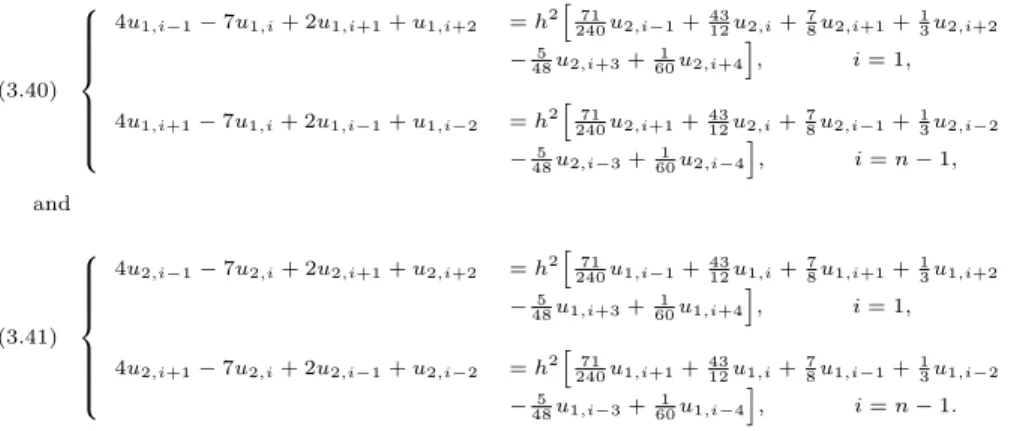
(3.40)                 

4u1,i−1−7u1,i+ 2u1,i+1+u1,i+2 =h2

h₇₁

240u2,i−1+4312u2,i+78u2,i+1+13u2,i+2 −5

48u2,i+3+601u2,i+4

i

, i= 1,

4u1,i+1−7u1,i+ 2u1,i−1+u1,i−2 =h2

h

71

240u2,i+1+4312u2,i+78u2,i−1+1₃u2,i−2 −5

48u2,i−3+601u2,i−4

i

, i=n−1,

and (3.41)                 

4u2,i−1−7u2,i+ 2u2,i+1+u2,i+2 =h2

h₇₁

240u1,i−1+4312u1,i+78u1,i+1+13u1,i+2 −5

48u1,i+3+601u1,i+4

i

, i= 1,

4u2,i+1−7u2,i+ 2u2,i−1+u2,i−2 =h2

h

71

240u1,i+1+4312u1,i+78u1,i−1+1₃u1,i−2 −5

48u1,i−3+ 1 60u1,i−4

i

, i=n−1.

The Eqs. (3.39)-(3.41) produce a linear system that contains 2×(n− 1) equations with 2×(n−1) unknown coefficients uj,i, j = 1,2, i = 1,2, . . . , n−1. Solving this linear system, we can obtain the approximate solution of the system of second-order boundary value problems (3.29).

Suppose kEu1(h)k∞and kEu2(h)k∞ be the maximum absolute errors.

We solved Example 3.2 for different values ofn. The maximum of absolute errors on the uniform grid points (3.24) are tabulated in Table 2. We compare the results with the SGM [23] applied to same equation. Table 2 exhibits the compared results.

Table 2. Our method for Example 3.2.

n kEu1(h)k∞ kEu2(h)k∞ kEu1(h)k∞−SGM[23] kEu2(h)k∞−SGM[23]

10 6.70171×10−10 6.70171×10−10 2.72950×10−4 2.72950×10−4

20 7.07034×10−12 7.07034×10−12 8.69675×10−6 8.69675×10−6

30 8.10463×10−13 8.10463×10−13 5.65263×10−7 5.65263×10−7

40 1.55653×10−13 1.55653×10−13 5.47391×10−8 5.47391×10−8

4. Conclusion

In this paper parametric quintic spline method employed for finding the extremum of a functional over the specified domain. The main pur-pose is to find the solution of boundary value problems which arise from the variational problems. The parametric quintic spline method reduce the computation of boundary value problems to some algebraic equations. The proposed scheme is simple and computationally attractive. Applica-tions are demonstrated through illustrative examples.

References

[1] R. Weinstock,Calculus of Variations: With Applications to Physics and Engineer-ing, Dover, 1974.

[2] B. Horn and B. Schunck, Determining optical flow, Artificial Intelligence, 17

(1981), 185–203.

[3] K. Ikeuchi and B. Horn,Numerical shape from shading and occluding boundaries, Artificial Intelligence,17(1981), 141–184.

[4] L. Elsgolts,Differential Equations and Calculus of Variations, Mir: Moscow, 1977 (translated from the Russian by G. Yankovsky).

[5] I.M. Gelfand and S.V. Fomin,Calculus of Variations, Prentice-Hall: Englewood Cliffs, NJ, 1963.

[6] C.F. Chen and C.H. Hsiao, it A walsh series direct method for solving variational problems, J. Franklin Inst.,300(1975), 265–280.

[7] R.Y. Chang and M.L. Wang,Shifted Legendre direct method for variational prob-lems, J. Optim. Theory Appl.,39(1983), 299–306.

[8] . I.R. Horng and J.H. Chou,Shifted Chebyshev direct method for solving variational problems, Internat. J. Systems Sci.,16(1985), 855–861.

[9] C. Hwang and Y.P. Shih,Laguerre series direct method for variational problems, J. Optim. Theory Appl.,39(1983), 143–149.

[10] S. Dixit, V.K. Singh, A.K. Singh and O.P. Singh, Bernstein Direct Method for Solving Variational Problems, International Mathematical Forum,5(2010), 2351– 2370.

[11] M. Razzaghi and S. Yousefi,Legendre wavelets direct method for variational prob-lems, Mathematics and Computers in Simulation,53(2000), 185–192.

[12] M. Tatari and M. Dehghan, The numerical solution of problems in calculus of variation using Chebyshev finite difference method, Physics Letters A372(2008), 4037–4040.

[13] J.H. Ahlberg, E.N. Nilson and J.L. Walsh,The Theory of Splines and Their Ap-plications, Academic Press: New York 1967.

[14] T.N.E. Greville, Introduction to spline functions, in: Theory and Application of Spline Functions, Academic Press: New York 1969.

[16] G. Micula and Sanda Micula,Hand Book of Splines, Kluwer Academic Publisher’s 1999.

[17] S.S. Siddiqi and G. Akram,Numerical solution of a system of fourth order bound-ary value problems using cubic non-polynomial spline method, Applied Mathemat-ics and Computation,190(2007), 652–661.

[18] M.A. Ramadan, I.F. Lashien and W.K. Zahra, Polynomial and nonpolynomial spline approaches to the numerical solution of second order boundary value prob-lems, Applied Mathematics and Computation,184(2007), 476-484.

[19] A. Khan,Parametric cubic spline solution of two point boundary value problems, Applied Mathematics and Computation,154(2004), 175–182.

[20] A. Khan and T. Aziz,Parametric cubic spline approach to the solution of a system of second-order boundary-value problems, Journal of Optimization Theory and Applications,118(2003), 45–54.

[21] J. Rashidinia, R. Jalilian and R. Mohammadi,Non-polynomial spline methods for the solution of a system of obstacle problems, Applied Mathematics and Compu-tation,188(2007) 1984–1990.

[22] J. Rashidinia, R. Jalilian and R. Mohammadi, Convergence analysis of spline solution of certain two-point boundary value problems, Computer Science and En-gineering and Electrical EnEn-gineering,16(2009), 128–136.

[23] M. Zarebnia and N. Aliniya ,Sinc-Galerkin method for the solution of problems in calculus of variations, International Journal of Engineering and Natural Sciences,

5(2011), 140–145.

M. Zarebnia

Department of Mathematics, University of Mohaghegh Ardabili, 56199-11367, Ardabil, Iran

Email: [email protected] Z. Sarvari

Department of Mathematics, University of Mohaghegh Ardabili, 56199-11367, Ardabil, Iran