Available online at http://pubs.sciepub.com/acis/2/3/2 © Science and Education Publishing
DOI:10.12691/acis-2-3-2
Robust Lead Compensator Design for an
Electromechanical Actuator Based on H∞ Theory
Rafik Salloum1,*, Mohammad Reza Arvan1, Bijan Moaveni2
1
Faculty of Electrical Engineering, Malek-Ashtar University of Technology (MUT), 15875-1774, Tehran, Iran
2
School of Railway Engineering, Iran University of Science and Technology (IUST), 16846-13114, Tehran, Iran *Corresponding author: [email protected]
Received July 01, 2014; Revised July 10, 2014; Accepted July 15, 2014
Abstract
In this paper, we design a robust lead compensator for a real Electromechanical Actuator (EMA) harmonic drive by introducing an approach based on H∞ control theory. Here, we address three main topics; experimental identification, uncertainty modelling, and robust control design for a real EMA harmonic drive system. This method verifies good tradeoff between the powerful H∞ controller and the unique features of compensators, such as: simplicity, low cost and easy implementation. The H∞ controller and the extracted compensator are almost identical within the EMA bandwidth range. Simulation and test results prove the effectiveness of the proposed approach and the superiority of the performance of the designed robust EMA with lead compensator based on H∞ controller over the original EMA; this preference is pertaining to its robustness to parametric uncertainties and high performance.Keywords
: Electromechanical actuator (EMA), identification, uncertainty modelling, robust control, leadcompensator, H∞ control theory
Cite This Article:
Rafik Salloum, Mohammad Reza Arvan, and Bijan Moaveni, “Robust Lead CompensatorDesign for an Electromechanical Actuator Based on H∞ Theory.” Automatic Control and Information Sciences,
vol. 2, no. 3 (2014): 53-58. doi: 10.12691/acis-2-3-2.
1. Introduction
Electromechanical actuators (EMA) are finding increasing use in the robotic and aerospace applications, since they have attractive characteristics such as: simplicity, reliability, low cost, good dynamic characteristics, and easy control [1,2].
Modelling and identification of the plant properly is the most effective step in control system design procedure. A good model is the simplest model that best explains the dynamics and successfully simulates or predicts the output
for different inputs [3]. However, EMA modeling is
subjected to uncertainty due to several reasons including operating point changes, perpetual parametric variations because of temperature changes, aging, unmodelled dynamics, and asymmetric behaviour. Consequently, the desired EMA's performance will be unachievable and, in some cases, its stability may be lost. Usually, based on experience, this problem will not be solved by using the conventional controllers; instead robust controllers with regard to the uncertainties in the model are needed to obtain the desired performance and stabilization demands in dealing with dynamic uncertainties [4].
Much effort is devoted to design robust controllers for uncertain systems based on different robust design methods known in literature such as Kharitonov's theorem,
small gain theorem, H∞, and Quantitative Feedback
Theory (QFT) [5,6,7]. Computational methods for
determining the set of all stabilizing controllers, of a given order and structure, for linear time-invariant delay free systems are reported in [8,9]. A graphical design method of tuning the PI and PD controllers achieving gain and phase margins is developed in [10,11]. Besides, in [12], the Kharitonov theorem is exploited for characterizing all PID controllers that stabilize an uncertain plant, also PID controllers design for systems without time delay were presented in [13,14]. H∞ theory based controller was designed to get faster and more accurate EMA system in
[15,16] and to improve the tracking and resolution of a
servo positioning system in [17]. But, a well-known
drawback of the H∞ controller, it is high order controllers and high computational cost.
In this paper, the EMA harmonic drive system is modelled as linear system with parametric uncertainty. In addition, the multiplicative uncertainty describing the deviation of the nominal model from the real EMA system due to the ignored nonlinearities is extracted. A method
based on H∞ theorem and Bode diagram is proposed to
design a lead compensator for the EMA system. This controller verifies good tradeoff between the powerful H∞ controller and the unique features of compensators.
validation is carried out in section 4. Finally, conclusion is stated.
2. Experimental Set-up
Our EMA consists of a DC motor with integrated harmonic drive gearing with 300:1 reduction ratio, driven by PWM power driver, and a potentiometer as position sensor fixed on the output shaft with coefficient of 0.5 Volt/deg, as shown in Figure 1. In this figure, r is the set point voltage, v is the PWM output, δ is the output angle, and δv is the angle measured by the potentiometer in volts. Here, r, v, and δv are acquired from experimental tests by a sampling time of 1 msec.
Figure 1. EMA harmonic drive scheme
3. System Identification and Uncertainty
Modelling
The objective of system identification is to find the approximate models of dynamic system based on knowledge of the observed input and output data to be used in uncertain modelling.
In this section, the linear model of the harmonic drive system is identified based on the test data. The captured data, related to several test sets at different conditions, were used for model estimation and validation purposes. The data of every set were divided into two portions: first one was used in the model estimation process (identification data), and the second was utilized in the validation process (validation data). The data captured from the real plant were used in the iterative
prediction-error estimation method (PEM) [18]. The discrete time
model is then transformed to continuous time model to be used in the uncertainty modelling.
3.1. System Identification
The input is the voltage to motor and the output is the potentiometer output. In this case, the PRBS signal cannot be used for identification since the test takes place in the open loop form and PRBS signal transfers the position sensor to saturation condition. Hence, the input signal for identification process is chosen to be a symmetric square wave and the output angle is measured from the potentiometer. But, to satisfy the persistent excitation (PE)
property, we prepare numbers of square waves with different frequencies and amplitudes for identification. Frequencies of square waves are chosen between 0 to 20 Hz and their amplitudes are chosen between 0.1 to 27 volts. These values are chosen based on the desirable bandwidth and operational conditions of motor, respectively. Seven imported data sets corresponding to different amplitudes were used for model identification. For instance, one test set results of the EMA harmonic drive system and its identified model are depicted in Figure 2.
The average error produced by a model is encapsulated in the mean squared error (MSE), which measures the precision of the estimated model. It is calculated as:
3.5 4 4.5 5 5.5
-1.5 -1 -0.5 0 0.5 1 1.5
MHD-Test # 3
Time [sec]
P
os
ti
on s
ens
or
out
put
[V
o
lt]
-.-.-.- Input ____ Measured --- Model; fit 82.2%
Figure 2. Measured data and identified model for the EMA harmonic drive system
( )
(
)
21
1
( , ) ( )
n
m m
i
MSE y y y i y i
n =
=
∑
− (1)where y is the actual (measured) output, ym is the output of
the model, and n is the number of data samples.
Furthermore, the model should attain best fitting to the measured data. The percentage of the output variation that is explained by the model is:
% 1 ym y 100%
fit
y y
−
−
= − ×
−
(2)
where y mean y
( )
−
= .
The identified models are tabulated with their MSEs and fitting percentages in Table 1.
3.2. Model Uncertainty Estimation
Considering the transfer functions for the identified
models tabulated in Table 1, the parametric uncertain
model was built to be used in H∞ robust controller design.
( )
( )
MHD
K
G s
s s q
=
+ (3)
[
]
[
]
582,1310 ; 961
56.5, 79 ; 61.4
nominal
nominal
K K
q q
∈ =
∈ =
The nominal model can be written as follows:
( )
961( 61.4)
nom
G s
s s
=
+ (4)
Table 1. Identification Results for the EMA HarmonicDrive System
Test set No. Model MSE Fitting (%)
1 1310
s(s+72.55) 0.0079 96.8
2 1187.4
s(s+63.86) 0.0034 95.7
3 636
s(s+64.85) 0.0079 82.2
4 582.6
s(s 56.5)+ 0.0072 86.2
5 1236
s(s+79) 0.0033 94.4
6 1308
s(s+76.91) 0.0032 96
7 655
s(s 57.45)+ 0.049 72
4. Robust Controller Design
In this section, a novel approach to design a robust lead compensator based on H∞ robust controller theory will be detailed. The overall philosophy in the design procedure presented here is to design a robust H∞ controller, then reduce its order maintaining its characteristics in the working frequency range, next it will be re-arranged to get the final compensator form.
4.1. System requirements
The required performance of the EMA system to be designed is a deadbeat response as shown in Table 2.
Table 2. Time DomainSystemPerformanceRequirements
Parameter Value
Rise time tr< 20 msec Settling time ts< 35 msec Steady-state position error 0
Overshoot < 1%
Consequently, the frequency domain system requirements may be derived from Table 2 as follows: The settling time constraint leads to minimum bandwidth 10 Hz. The overshoot constraint (< 1%) assigns the minimum damping ratio to 0.826, and the minimum phase margin should be 40 deg.
4.2.
H∞ Robust Controller Design
H∞ theory presents powerful frequency-domain
framework for capturing control design requirements such as bandwidth, response speed, robust stability, and
disturbance rejection [19]. The EMA system in H∞
framework is illustrated in Figure 3.
Figure 3. EMA system in H∞ framework
K is the robust controller, G: Motor and harmonic drive system, r: command reference signal, u: control signal, e:
tracking error, and y: plant output. Define the error
sensitivity function S= +(1 GK)−1 , the control signal
sensitivity function U=K(1+GK)−1 , and the
complementary sensitivity function T =GK(1+GK)−1. Robust performance constraint: W Se ∞ ≤1
Robust Stability constraint: WT ∞ ≤1
Control signal (saturation) constraint: W Uu ∞≤1
W, Wu and We are frequency dependent weighting functions.
The objective is to find controller K that stabilizes Gnom and satisfies H∞ norm of a transfer matrix consisting of weighting functions is smaller than one, i.e.:
1.
e
u
W S W U
WT ∞
≤ This problem is called mixed sensitivity
problem [19].
Here, we consider the multiplicative uncertainty to describe the deviation of the nominal model from the real system due to the ignored nonlinearities in real system.
Assume GMHD is the models of the motor and harmonic
drive, identified from the test sets tabulated in Table 1, and Gnom is the nominal model. Using the multiplicative uncertainty definition:
( )
(
1( ) ( )
)
( )MHD nom
G s = + ∆ s W s G s (5)
where W(s) is the uncertainty weighting function, and Δ is
an operator with infinity-norm less than unity [20], i.e.
( )s ∞ 1
∆ < , so
( )
( )
( )
( )
,MHD nom
nom
G j G j
W j
G j
ω ω
ω ω
ω −
≤ ∀ (6)
By plotting the frequency response of
( )
( )
( )
MHD nom
nom
G j G j
G j
ω ω
ω −
, the multiplicative uncertainty
weighting function can be extracted from the upper bound of different uncertainty frequency plots of the identified uncertain system; they are shown in Figure 4. The multiplicative uncertainty weighting function is approximated by:
( )
110275
s W s = +
10-2 100 102 104 -70
-60 -50 -40 -30 -20 -10 0 10 20 30
M
agni
tude (
dB
)
Bode Diagram
Frequency (rad/sec)
Dashed: System variations |(G-G0)/G0| Solid: Uncertainty weighting function W
Figure 4. Uncertainty and weighting function frequency responses; simulation
It may be concluded from Figure 4 that the uncertainty at low frequencies is small (about -7.5 dB), which allow robust control of the EMA system within this bandwidth.
W is the robustness weighting function to be used in H∞
robust controller design. Use of this identified uncertainty model in the robust control design procedure decreases the deviations between designed model performance and experimental results [21].
The sensitivity weighting function is assigned to:
( )
0.1 5031.2
50 10
e
s W s
s −
+
= ×
+ ×
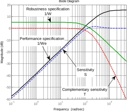
which indicates sensitivity reduction of 100:1 (- 40 dB) for frequencies up to 1 rad/sec (i.e. at low freq. the closed loop should reject disturbance at the output by a factor of 100 to 1 or the steady state tracking errors due to step input should be less than 1%), as depicted in Figure 5.
10-1 100 101 102 103
-60 -50 -40 -30 -20 -10 0 10 20
M
agni
tude (
dB
)
Bode Diagram
Frequency (rad/sec)
Complementary sensitivity T
Sensitivity S Performance specification
1/We
Robustness specification 1/W
Figure 5. Closed loop sensitivity, complementary sensitivity, robustness and performance functions with H∞ controller; simulation
The control signal sensitivity weighting function Wu (the actuator saturation weighting function) is chosen considering the physical limitation of the EMA. Thus, it can be considered to be a constant, so that the maximum expected input r (2 volt in this case) never saturates the actuator (saturation voltage 27 volt). Its value is estimated to be: Wu = 0.02.
The H∞ controller, designed by Matlab and verifying
H∞cost γ = 0.721, is:
163938.5s(s 61.4) ( 4603)( 342.4)(s 0.05)
K
s s
+ =
+ + + (7)
Since the H∞-norm of the closed-loop system is less
than one, the condition: WT ∞ ≤1 is satisfied in the
given case. This may be checked by computing the sensitivity function of the closed-loop system and comparing it with the inverse of the performance weighting function. The result of the comparison is shown in Figure 5. It is seen that the sensitivity function lies below 1/We.
Similarly, the condition WT ∞≤1 may be checked by
computing the complementary sensitivity function of the closed-loop system and comparing it with the inverse of therobustness weighting function. The result of the comparison is shown in Figure 5, where the complementary sensitivity function lies beneath 1/W.
4.3. Compensator Derivation
16 18 20 22 24 26 28 30
M
agni
tude (
dB
)
10-1 100 101 102
0 5 10 15 20 25 30 35 40 45
P
has
e (
deg)
Bode Diagram
Frequency (Hz)
Lead Compensator
Hinf Controller
Figure 6. H∞ controller and the reduced one; simulation
Low order controllers are normally preferred over high order controllers in control system since they are computationally less demanding; easier to implement and they have higher reliability due to fewer things to go
wrong in the hardware [22]. The dc-gain of EMA system
plays an important role in assessing its performance, for this reason it should be maintained. The 3rd order designed
H∞ controller will be reduced in a manner to keep its
characteristics in the working frequency range using balanced residualisation (singular perturbation approximation) method which gives best approximation at low frequencies [23].
( )
35.6(s 61.4) (1 ) ( 342.3) (1 )red
Ts
K s A
s Ts
α
+ +
= =
+ + (8)
which is a lead compensator with A = 35.6, α = 5.58, and
T = 2.92 x 10⁻³. Figure 6 shows that the H∞ and the reduced order controllers are almost identical in the range
below 100 Hz which is sufficiently wider than our
of resistors, capacitors, transistors, diodes and op-amps
[24].
4.4. Compensator Realization
The lead compensator is realized by active components circuit shown in Figure 7.
Figure 7. Designed compensator circuit
The compensator transfer function is:
( )
35.6(s 61.4) ( 342.3)red
K s
s
+ =
+ (9)
From the circuit diagram shown in Figure 7, R1, R2 and
C form the compensator network where as Rf and R0 form the compensator gain (A). The transfer function from the input voltage to the controller V1 to the output voltage V2 is:
2 1
1 2
1
1 2
1
s
V R C
R R
V s
R R C
+ =
+
+ (10)
Op-Amp: TL074, R1= 162 KΩ, C = 0.1 μF and R2= 36 KΩ.The constant gain A = 35.6 is verified by the used compensator circuit in Figure 7; this is given by:
0 0
1 Rf 35.6; f 34.6 Ω; 1 Ω
A R K R K
R
= + = = =
4.5. Performance Validation of the Robust
EMA with H∞ derived Compensator
Table 3 illustrates the time response values for the H∞
controller and the derived lead compensator, which clarify that there is no considerable performance retreat.
Table 3. Characteristics of Robust EMAs with H∞Controller and Derived Compensator
Model tr(msec) ts(msec) Over-shoot(%)
S. S. Error Robust EMA with H∞
controller 15.7 26 0.08 0
Robust EMA with reduced order H∞ (lead
compensator)
16.2 26.9 0.05 0
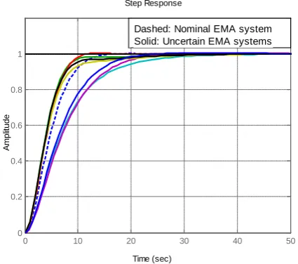
The step responses and bode plots of the uncertain closed loop EMA syetem with the derived lead compensator are depicted in Figure 8 and Figure 9, respectively.
0 10 20 30 40 50
0 0.2 0.4 0.6 0.8 1
Step Response
Time (sec)
A
m
pl
itude
Dashed: Nominal EMA system Solid: Uncertain EMA systems
Figure 8. Step responses of nominal and uncertain closed loop EMA with the derived lead compensator; simulation
Bode Diagram
Frequency (Hz)
10-1 100 101 102
-20 -15 -10 -5 0 5
System: untitled4 Frequency (Hz): 12.2 Magnitude (dB): -3
M
agni
tude (
dB
)
Dashed: Nominal system Solid: Uncertain systems
Figure 9. Closed loop frequency response for nominal and uncertain EMA with the lead compensator; simulation
The new designed EMA system with lead compensator
derived from the H∞ controller, in addition to its
robustness to parametric uncertainties, has almost the
same dynamics of the H∞ controller and the simplicity
advantages of compensators.
In order to verify that other system requirements in
Table 2 are met with the derived compensator, the margins and bandwidths were tabulated in Table 4.
40 90 140 180
0 5 10 15 20 25 30
Time [msec]
C
ont
rol
s
ignal
[
v
ol
t]
Lead-compensator controller
Hinf controller
Table 4. Margins of Uncertain Plants with the Compensator
TF Gain margin (dB) Phase margin (deg) Bandwidth (Hz)
Gnom 33.9 73.1 21
G1 31.5 72.7 26.9
G2 32.1 70.8 25
G3 37.6 80.4 14.2
G4 38.1 76.6 13.5
G5 32.2 76.6 25.1
G6 31.6 74.5 26.5
G7 37.1 76 15
It is noted that system requirements are verified. The control signal may be checked so that the actuator will not be saturated during operation. The control signals to the actuator corresponding to maximum input command (2 volts) with the designed robust controllers were plotted (as illustrated in Figure 10).
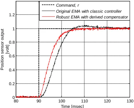
Finally, the performance of the robust EMA with H∞
derived compensator was compared with the original classic controller EMA performance. It proves, in addition to its robustness to parametric uncertainties, better dynamic performance, as shown in Figure 11.
80 90 100 110 120 130
0 0.2 0.4 0.6 0.8 1 1.2
Time [msec]
P
os
it
ion s
ens
or
out
put
[v
o
lt]
Command, r
Original EMA with classic controller Robust EMA with derived compensator
Figure 11. Measured step for original and robust EMA systems; experiment
5. Conclusion
An approach to design robust compensator, based on
H∞ theory, was applied on an EMA harmonic drive system. It leaded to a robust EMA system which is, in addition to its robustness, simple and easily implementable.
The robust controller design and validation procedure is studied by simulation and experiments, and its effectiveness is proven by comparing the performance of compensator with the robust H∞ controller and the original EMA system with classic controller. The comparison has demonstrated the effectiveness of the proposed robust EMA system with lead compensator.
The proposed approach applied on the EMA system, may be applied on other control systems operating over a relatively low range of frequencies.
References
[1] Ristanović, M., Ćojbašić, Ž. and Lazić, D., “Intelligent control of DC motor driven electromechanical fin actuator,” J. Control Engineering Practice, 20 (6). 610-617. Mar. 2012.
[2] Liscouët, J., MaréJ. C. and Budinger, M., “An integrated methodology for the preliminary design of highly reliable electromechanical actuators: Search for architecture solutions,”
Aerospace Science and Technology, 22 (1). 9-18. Oct-Nov. 2012. [3] Walter, E., Pronzato, L. and Norton, J., Identification of
Parametric Model from Experimental Data, Springer, GB, 1997. [4] Lu, H., Li, Y. and Zhu, C., “Robust synthesized control of
electromechanical actuator for thrust vector system in spacecraft,”
J. Computers and Mathematics with Applications, 64 (5). 699-708. Sept. 2012.
[5] Toscano, R., “A simple robust PI/PID controller design via numerical optimization approach,” J. of process control, 15 (1). 81-88. Feb. 2005.
[6] ValérioD. and Costa, J., “Tuning of Fractional Controllers Minimising H2 and H∞ Norms,” Acta Polytechnica Hungarica, 3 (4). 55-70. 2006. [7] Yogesh, V. H., Gupta, J. R. P. and Choudhury, R., “Kharitonov’s
Theorem and Routh Criterion for Stability Margin of Interval Systems,” International Journal of Control, Automation, and Systems, 8 (3). 647-654. June 2010.
[8] Saadaoui, K. and Özgüler, A. B., “A new method for the computation of all stabilizing controllers of a given order,”
International Journal of Control, 78 (1). 14-28. Jan. 2005. [9] Tantaris, R. N., Keel, L. H. and Bhattacharyya, S. P.,
“Stabilization of discrete-time systems by first-order controllers,” IEEE Trans. Automat Control, 48 (5). 858-861. May 2003. [10] Tan, N., “Computation of stabilizing PI-PD controllers,”
International Journal of Control, Automation, and Systems, 7 (2). 175-184. April 2009.
[11] Yeroglu, C. and Tan, N., “Design of Robust PI Controller for Vehicle Suspension System,” Journal of Electrical Engineering & Technology, 3 (1). 135-142. 2008.
[12] Huang, Y. J. and Wang, Y.-J., “Robust PID tuning strategy for uncertain plants based on the Kharitonov theorem,” ISA Transactions, 39 (4). 419-431. Sept. 2000.
[13] Li, X. H., Yu, H.B., Yuan, M.Z. and Wang, J., “Design of robust optimal proportional-integral-derivative controller based on new interval polynomial stability criterion and Lyapunov theorem in the multiple parameters’ perturbations circumstance,” IET Control Theory Appl., 4 (11). 2427-2440. Nov. 2010.
[14] Rigatos, G. and Siano, P., “Design of robust electric power system stabilizers using Kharitonov’s theorem,” Mathematics and Computers in Simulation, 82 (1). 181-191. Sept. 2011.
[15] Yoo, C.-H., Lee, Y.-C. and Lee, S.-Y., “A Robust Controller for an Electro-Mechanical Fin Actuator,” in Proceeding of the American Control Conference, Boston, Massachusetts, 5, June 30-July 2, 2004, 4010-4015.
[16] Benderradji, H., Chrifi-Alaoui, L., Mahieddine-Mahmoud S. and Makouf, A., “Robust Control of Induction Motor with H∞ Theory based on Loopshaping,” Journal of Electrical Engineering & Technology, 6 (2). 226-232. 2011.
[17] Raafat, S. M., Akmeliawati, R. and Abdulljabaar, I., “Robust H∞ Controller for High Precision Positioning System, Design, Analysis, and Implementation,” Intelligent Control and Automation, 3 (3). 262-273. Aug. 2012.
[18] Ljung, L., System Identification: Theory for the User, 2nd edition, Prentice-Hal PTR, Upper Saddle River, NJ, 1999.
[19] Bhattacharyya, S. P., Chapellat, H. and Keel, L. H., Robust Control: The Parametric Approach, Prentice Hall, 1995.
[20] Tavakoli, M., Taghirad, H. D., and Abrishamchian, M., “Identification and Robust H∞ Control of the Rotational/Translational Actuator System,” International Journal of Control, Automation, and Systems, 3 (3). 387-396. Sept. 2005. [21] Lim, K. B., Cox, D. E., Balas, G. J. and Juang, J.-N., “Validation
of an Experimentally Derived Uncertainty Model,” Journal of Guidance, Control, and Dynamics, 21 (3). 485-492. May-June 1998. [22] Zhou, K., Doyle, J. C. and Glover, K., Robust and Optimal
Control, Prentice Hall, Englewood Cliffs, New Jersey, 1996. [23] Oh, D. C., Bang, K. H. and Park, H. B., “Controller order
reduction using singular perturbation approximation,” Automatica, 33 (6). 1203-1207. June 1997.