Available online throug
ISSN 2229 – 5046PERSISTENCE AND OPTIMAL HARVESTING
OF MARINE POPULATION AFFECTED WITH PRIMARY AND SECONDARY TOXICANT
PRAGYA MISHRA
1, RACHANA PATHAK*
2, MANJU AGARWAL
31
Govt. P. G. College, Hardoi, India.
2,3
Department of Mathematics & Astronomy, Lucknow University, Lucknow, India.
(Received On: 09-10-15; Revised & Accepted On: 28-10-15)
ABSTRACT
T
his work investigates the affect of toxicant which is structured into two stages, primary and secondary on a single species fishery model. Boundedness and positivity of solution has been shown in order to ensure feasibility of biological model. The time lag required for transmission of primary toxicant to secondary toxicant is incorporated and resulting delayed model is analyzed for stability. Optimal harvesting policy has been discussed by using Pontryagin’s Principal. Butler-Mc Gehee lemma is used to identify the condition which influences the persistence of the system. Finally, some numerical simulations are given to verify the mathematical conclusions.Keywords: Stability, Time-delay, Optimal harvesting, Persistence.
1. INTRODUCTION
With the rapid development of modern technology, industry and agriculture, a large quantity of toxicant and contaminants enter into the ecosystem one after another. These toxicants seriously threaten the survival of the exposed population. In order to regulate toxic substances wisely, we must assess the risk of the population exposed to toxicant. Therefore, it is important to study the effects of toxicant on biological population and to find a theoretical threshold value, which determines permanence or extinction of biological population.
In recent years, some investigations have been conducted to study the effect of toxicant emitted into the environment from industrial and household resources on biological species by using mathematical models. In particular, Hallam et.al. [2–5] in series of their papers studied qualitative approach of toxicants on population. They assumed growth rate density of single species as decreasing function of toxicant concentration whereas carrying capacity is taken as constant.
Freedman and Shukla in their paper [1] studied the effect of toxicant on a single species and on a prey–predator community by taking into account the introduction of toxicant from an external source and both growth rate and carrying capacity are taken as decreasing function of toxicant. They assumed the same nature of toxicant and not taken into consideration different stages of toxicant. But in reality, we can structure toxicant according to its level of intensity or according to its chemical composition. Since in some cases, toxicant at low intensity level does not effect the growth of biological species but when its intensity is increased, it affects the biological population adversely. One example is the emission of carbon and sulphur dioxide through industries and vehicles. These pollutants do not affect fishery habitat in initial stage but in more toxic stage, in the form of acid rain these pollutant affect the growth of marine ecosystem seriously.
Shukla et al. [6] studied the effects of primary and secondary toxicants on resource biomass. They showed that the decrease in biomass density of resource is more than one, in corresponding case of a single toxicant due to large transformation, uptake rates and high toxicity of secondary toxicant.
Corresponding Author: Rachana Pathak*
2Keeping the above thing in mind, we propose a fishery model to discuss the effects of primary (low intensity) and secondary (more toxic) toxicant on the stability and harvesting of marine species. The organization of paper is as follows : Section 2 deals with the mathematical model and some basic results on positivity and boundedness of the system. In section 3 existence of equilibrium points and their stability behaviour is discussed in the absence of delay. The critical value of delay is calculated at which stability change can occur and occurrence of Hopf bifurcation. Optimal harvesting policy is discussed in section 4. In Section 5, we derive the sufficient conditions for persistence and numerical simulations are included to illustratre the applicability of the results obtained in Section 6, and lastly discussion is presented in Section 7.
2.THE MATHEMATICAL MODEL
We consider a single species fishery model with toxicant affect governed by following differential equations:
(
,
)
1
( )
,
2 1
2
qxE
T
K
x
x
T
T
r
dt
dx
−
−
∈
=
(
) (
,
1)
,
1 1 1 0 1
T
x
h
t
T
T
Q
dt
dT
∈
−
−
−
−
=
α
β
τ
(1)(
)
2 2(
,
2)
,
1 2
T
x
g
T
t
T
dt
dT
θβ
τ
α
γ
−
−
−
=
with initial conditions
( )
0
>
0
,
T
1( )
t
=
1( )
t
>
0
,
T
2( )
t
=
2( )
t
>
0
x
φ
φ
for−
τ
≤
t
≤
0
.
Here
x
( )
t
is the concentration of single fish species,T
1( )
t
is the concentration of primary toxicant that is of lowintensity and
T
2( )
t
is highly toxic secondary toxicant concentration at any timet
>
0
. In modelling the system (1), we made following assumption:H1: The fish population grows logistically with its secondary toxicant dependent carrying capacity
K
( )
T
2 and toxicantdependent growth function
r
(
T
2,
∈
T
1)
. It is assumed that growth is slightly affected by primary toxicant i.e.1
∈<<<
. These functions satisfy the following properties:( )
( )
( )
0 2 2
0 1 2
2 1
0
0,
'
0
0,
0
0,
0,
0, ,
0,
K
K
K T
T
r
r
r
r
T T
T
T
=
>
<
∀ >
∂
∂
= >
<
<
∀
>
∂
∂
there exists some values of
T
1andT
2 such that( )
T
2=
0
,
r
(
T
~
2,
∈
T
~
1)
=
0
.
K
H2: The fish population is harvested with constant harvesting effort
E
in direct proportion to its concentration withconstant catchability coefficient
q
>
0
.
H3: The primary toxicant is emitted into the environment with a prescribed rate
Q
0 by an external source andtransmitted into highly toxic form after time
τ
with toxicant dependent conversion function asθβ
T
1(
t
−
τ
)
whereβ
is constant conversion rate which converted into secondary toxicant from primary toxicant.H4: In the absence of toxicant, when 0
−
<
0
,
<
0
,
dt
dx
qE
r
and fish population approaches to extinction. So throughoutin this paper, we assume
r
0−
qE
>
0
.H5 : The uptake of primary and secondary toxicant by the population is presented by increasing functions
h
(
x
,
T
1)
and(
x
,
T
2)
g
respectively :(
,
) ( )
,
0
0
,
0
,
0
,
1
1
∂
>
∂
>
∂
∂
=
=
T
h
x
h
x
h
T
x
h
(
0,
2)
( )
, 0
0,
0,
0
, ,
1 20.
g
g
g
T
g x
x T T
x
T
∂
∂
=
=
>
>
∀
>
The constants
α
1 andα
2are depletion rate coefficients of primary and secondary toxicant respectively due to various factors in the environment. For simplicity, we assume simplest form of the functions as below:(
,
1)
1, 0
1
h x T
=∈
xT
<∈<<<
is the constant uptake coefficient of primary toxicant by the population.(
,
2)
2, 0
g x T
=
γ
xT
γ
>
is the proportionality constant for the uptake of secondary toxicant by the population.Then the system (1) takes the form
(
,
)
1
( )
,
2 1
2
qxE
T
K
x
x
T
T
r
dt
dx
−
−
∈
=
(
)
1,
1 1 1 0 1
xT
t
T
T
Q
dt
dT
∈
−
−
−
−
=
α
β
τ
(2)(
)
2 2 2,
1 2
xT
T
t
T
dt
dT
θβ
τ
α
γ
−
−
−
=
with initial condition
( )
0
>
0
,
T
1( )
t
=
1( )
t
>
0
,
T
2( )
t
=
2( )
t
>
0
x
φ
φ
for−
τ
≤
t
≤
0
.
Next, we have theorems regarding the positivity and boundedness of solutions of system (2).
Theorem 1: All solutions of the system (2) with initial conditions are non–negative.
Proof: Let
t
=
t
1 be the first time whenT
1( )
t
1=
0
.
Sot
1=
{
min
t
>
0
,
T
1( )
t
=
0
}
,
then 1 0 1
(
1)
0
,
1
>
−
−
=
=
τ
β
T
t
Q
dt
dT
t t
(since concentration of emitted toxicant should be sufficiently greater than transmitted toxicant). Hence for sufficiently
small
η
1>
0
,
T
1(
t
1−
η
1)
>
0
.
But by definition oft
1,T
1(
t
1−η
1)
≤
0
.
, this contradiction proves that( )
0
0
1
t
>
∀
t
>
T
.Similarly, lett
2=
{
min
t
>
0
,
T
2( )
t
=
0
}
,
then 2 1(
2)
0
.
2
>
−
=
=
τ
β
T
t
dt
dT
t t
Hence for
sufficiently small
η
2>
0
,
T
2(
t
2−
η
2)
>
0
.
But by definition oft
2,T
2(
t
2−η
2)
≤
0
.
again contradiction provesthat
T
2( )
t
>
0
∀
t
>
0
and also0
0
=
=x
dt
dx
proves the non–negativity of
x
( )
t
.
Hence, all solutions of system (2) are non–negative.
Theorem 2: The region
(
)
( )
( )
(
)
∈
≤
+
≤
=
=
Ω
+ 1 20 2
1 3
2
1
,
:
0
,
min
,
,
α
α
α
α
Q
t
T
t
T
R
T
T
x
is a region of attraction for all solutions initiating in the positive octant.
Proof: From system (2)
.
1
0
0
−
≤
K
x
x
r
dt
dx
On integrating and taking limit
t
→
∞
( )
t
K
0.
x
≤
Also 1 2 0
(
1 2)
,
T
T
Q
dt
dT
dt
dT
+
−
≤
+
α
where
α
=
min
(
α
1,
α
2)
. According to comparison principle, it follows that 0.
2
1
α
Q
T
3. THE MATHEMATICAL ANALYSIS
Existence of Equilibriums: The system (2) has only two non-negative equilibrium points namely
(
0
,
T
1,
T
2)
P
andP
*
(
x
*,
T
1*,
T
2*
)
.(
0
,
T
1,
T
2)
P
is given by(
)
.
,
1 2 0 2 1 01
α
α
β
θβ
β
α
+
=
+
=
Q
T
Q
T
Interiorequilibrium point
P
*
(
x
*,
T
1*,
T
2*
)
is given by the solution of following algebraic equations:(
,
)
1
( )
0
,
2 1
2
−
=
−
∈
qE
T
K
x
T
T
r
(3a),
0
1 1 1 10
−
T
−
T
−
∈
xT
=
Q
α
β
(3b).
0
2 2
2
1
−
T
−
xT
=
T
α
γ
θβ
(3c)From eqs. (3b) and (3c), we get
( )
(
)(
)
( )
.
*
,
*
2 2 1 0 2 1 1 0 1x
f
x
x
Q
T
x
f
x
Q
T
=
+
∈
+
+
=
=
∈
+
+
=
γ
α
β
α
θβ
β
α
Using the values of
T
1*
and
T
2*
in eq. (3a), we get( )
(
( )
,
( )
)
1
(
( )
)
,
2 1 2
qE
x
f
K
x
x
f
x
f
r
x
F
−
−
∈
=
( )
0
r
(
f
2( )
0
,
f
1( )
0
)
qE
,
F
=
∈
−
( )
(
( )
,
( )
)
1
(
( )
)
0
,
0 2 0 0 1 0 2
0
−
<
−
∈
=
qE
K
f
K
K
K
f
K
f
r
K
F
since
K
0>
K
(
f
2( )
K
0)
.
So, there exists an unique
x
*
such that0
<
x
*
<
K
0andF
( )
x
*
=
0
,
whenF
( )
0
.
>
0
,
andF
'
( )
x
<
0
.
From above analysis, we observe following points about the equilibrium points:
1. The three eigenvalues of variational matrix
M
1arer
(
T
2,
∈
T
1)
−
qE
,λτ
β
α
−
−−
1e
and−
α
2.Theequilibrium point
P
is stable inT
1−
T
2 plane and saddle point inx
−
T
1−
T
2 plane if(
T
T
)
qE
r
2,
∈
1>
.2. The characteristic equation corresponding to interior equilibrium
P
*
(
x
*,
T
1*,
T
2*
)
is given by(
2 3)
0
,
2 1 3 2 2 1
3
+
+
+
+
−+
+
=
b
b
b
e
a
a
a
λ
λ
λ
λ
λ
λτ(4)
where
(
)
( )
2 1(
)
1 1 2
2
*
*,
*
*,
*
x r T
T
a
x
K T
α α
γ
∈
=
+
+
+ ∈ +
(
)
( )
(
(
)
)
(
)(
)
( )
2 12 1 2 2 1
2
1 2
1 * 2
*
*,
*
*
*
*
*
*
*
* 1
*
*,
*
P
x r T
T
a
x
x
x
K T
r
x
x T
T
H
T
K T
α α
γ
α
γ
α
γ
∈
=
+
+ ∈ +
+
+
+ ∈
+
∂
∈
−
+
∂
(
)
( )
(
)(
)
(
*
)
*
*
(
*
)
,
*
*
*
*
*
*
*,
*
1 2 2 1 * 1 1 2 2 1 2 3x
H
T
x
T
x
T
r
x
x
T
K
T
T
r
x
a
P∈
+
+
+
∂
∂
∈
+
∈
+
+
∈
=
α
γ
γ
α
α
γ
α
(
)
( )
*
,
*
*
*,
*
,
2 2 1 2 2 1
+
+
∈
=
=
x
T
K
T
T
r
x
b
b
β
β
α
γ
(
)
( )
(
*
)
*
*
*
*
,
*
*
*,
*
2 1 2 2 1 2 3
+
∈
+
+
∈
=
x
H
T
H
T
T
K
T
T
r
x
b
β
α
γ
θ
γ
where
( )
(
( )
)
( )
.
*
*
'
*
*
*,
*
*
1
*
*
2 2 2 2 1 2 22 *
K
T
T
K
x
T
T
r
T
K
x
x
T
r
H
P∈
+
−
∂
∂
=
When
τ
=
0
,
i.e. in case of instantaneous transmission of primary toxicant into secondary toxicant, characteristic equation becomes(
)
(
2 2)
3 30
.
2 1 1
3
+
+
+
+
+
+
=
b
a
b
a
b
a
λ
λ
λ
(5)Since
a
1+
b
1>
0
,
whena
3+
b
3>
0
,
and(
a
1+
b
1)(
a
2+
b
2) (
>
a
3+
b
3)
,
then by Routh–Hurwitz criterion allroots of eq. (5) have negative real parts and
P
*
is locally asymptotically stable equilibrium point in the absence of delay.When
τ
≠
0
, stability of system can change only if there exists at least one root of eq. (4) such thatRe
( )
λ
=
0
. Letiw
=
λ
be one such root. Substituting this in eq. (4) and on equating real and imaginary parts, we have(
)
cos
sin
2 3,
1 2
3 2
1
w
b
w
b
w
w
a
w
a
b
−
τ
−
τ
=
−
+
(6)(
)
sin
cos
3 2.
2 3
2
1
w
b
w
b
w
w
w
a
w
b
−
τ
+
τ
=
−
(7)On squaring and adding these two equations, we get
(
2
)
(
2
2
)
20
.
3 2 3 2 3 1 2 2 3 1 2 2 4 2 1 2 2 1
6
+
−
−
+
−
−
+
+
−
=
b
a
w
b
b
b
a
a
a
w
b
a
a
w
(8)On substituting 2
,
u
w
=
in above equation(
2
)
(
2
2
)
20
.
3 2 3 3 1 2 2 3 1 2 2 2 2 1 2 2 1
3
+
−
−
+
−
−
+
+
−
=
b
a
u
b
b
b
a
a
a
u
b
a
a
When
P
*
is locally asymptotically stable equilibrium point in the absence of delay and following inequalities hold0
,
0
2
2 3 2 3 2 1 2 21
−
a
−
b
>
a
−
b
>
a
and(
2
)(
2
2
)
2,
3 2 3 3 1 2 2 3 1 2 2 2 1 2 2
1
a
b
a
a
a
b
b
b
a
b
a
−
−
−
+
+
>
−
(10) then all conditions of Routh Hurwitz criteria for the existence of negative roots are satisfied. Hence, the eq. (9) has only negative real roots and there exist no real solution of eq. (8), soP
*
remains stable for allτ
>
0
.Again on solving eqs. (6) and (7), we get a critical value of delay that is given as follows :
(
)(
)
(
)
(
)
,
b
sin
1
2 2 2 2 3 2 1 3 2 1 2 2 3 3 2 1 1
+
−
−
+
−
−
=
−w
b
b
w
a
w
a
w
b
w
a
w
b
w
b
w
cτ
this is the least positive value of delay for whichstability change occur.
4. OPTIMAL HARVESTING POLICY
In the present section, we discuss the optimal policy that should be adopted by regulatory agency in order to maximize net revenue. That is given by
(
pqx
−
c
)
E
.
=
π
(11)Our objective is to maximize following integral
( )
(
) ( )
,
0∫
∞ −−
=
e
pqx
t
c
E
t
dt
J
δtsubject to state equations of system (2) and to control constraint
q
r
E
E
0max
0
≤
≤
=
. Hereδ
is the instantaneousannual rate of discount,
p
is the price per unit biomass of landed fish andc
is fishing cost per unit effort.The associated Hamiltonian is given by
(
)
(
)
( ) (
)
( )
( )
[
]
( )
[
]
,
1
,
,
,
,
2 2 2 1 3 1 1 1 1 0 2 2 1 2 1 2 1xT
T
T
t
xT
T
T
Q
t
qxE
T
K
x
x
T
T
r
t
E
c
pqx
e
t
T
T
x
H
tγ
α
θβ
λ
β
α
λ
λ
δ−
−
+
∈
−
−
−
+
−
−
∈
+
−
=
− (12)where
λ
1,
λ
2 andλ
3are adjoint variables.The necessary condition for
E
*
to be optimal over the control set0
≤
E
*
≤
E
maxis=
0
,
∂
∂
E
H
which implies(
)
.
1E
e
c
pqx
e
qx
t t∂
∂
=
−
=
− −π
λ
δ δ(13)
So, the user’s cost of harvest per unit of effort equals the discounted value of the future marginal profit of the effort at the steady state level.
According to the Pontryagin’s Maximum principle, the adjoint variables
λ
1,
λ
2 andλ
3must satisfy.
,
,
2 3 1 2 1T
H
dt
d
T
H
dt
d
x
H
dt
d
∂
∂
−
=
∂
∂
−
=
∂
∂
−
=
λ
λ
λ
On considering interior equilibrium
P
*
(
x
*,
T
1*,
T
2*
)
and solving above equations we get( )
,
( )
,
( )
,
1 2 3 1 2 2 1 2 1 t t te
A
A
t
e
B
B
t
e
C
C
t
δ δ δδ
λ
δ
λ
δ
λ
− − −+
=
+
=
+
=
where( )
(
( )
)
*
( )
,
*
'
*
*
*,
*
*
1
*
*
*,
2 2 2 2 1 2 2 2 2 2 1
∈
+
−
∂
∂
−
=
+
=
T
K
T
K
x
T
T
r
T
K
x
x
T
r
qx
c
p
A
x
( )
(
( )
)
,
*
*
*,
,
*
*
1
*
T
r
*
*,
2 1 2 1 1
2 2
* 1 2
1 1
T
K
T
T
r
C
A
A
T
K
x
x
qx
c
p
B
x
B
P
∈
=
+
+
−
∂
∂
−
=
∈
+
+
=
δ
θβ
β
α
.
*
*
1 2 2 1
1 2
2
δ
γ
δ
−
+
+
∈
−
=
A
T
A
B
T
B
pqE
C
On equating two values of
λ
1( )
t
we get,
*
1 2
qx
c
p
C
C
−
=
+
δ
(14)this expression gives the optimal equilibrium level of species i.e.
x
δ, then the optimal equilibrium levels of both toxicants and harvesting effort are given by(
)(
)
,
(
,
)
1
( )
.
,
2 1
2 2
1
0 2
1 0
1
−
∈
=
+
∈
+
+
=
∈
+
+
=
δ δ δ
δ δ
δ δ
δ δ
δ
α
β
α
γ
θβ
β
α
K
T
x
q
T
T
r
E
x
x
Q
T
x
Q
T
It has been noted from above analysis that
( ) (
t
e
ti
=
1
,
2
,
3
)
iδ
λ
is independent of time and remains bounded ast
tends to infinity, so they satisfy transversality condition.From eq. (14), we observe that
0
*
*
1
2
→
+
=
−
δ
C
qx
C
c
pqx
asδ
→
∞
,
this shows that the economic rent is completely dissipated when discount rateis infinite.
5. PERSISTENCE
Theorem 5.1: Let
r
(
T
2,
∈
T
1)
>
qE
holds, then the system (2) persists (does not persist) ifP
*
exist (does not exist).Proof: To prove this theorem, we have to show that there are no omega limit points on the axes of orbits initiating in the interior of positive octant. Suppose
u
is a point in the positive octant andθ
( )
u
is the orbit throughu
andω
is the omega limit set of the orbit throughu
.Note thatω
( )
u
is bounded.We claim that
P
does not belong toω
( )
u
. IfP
∈
ω
( )
u
, the conditionr
(
T
2,
∈
T
1)
>
qE
implies thatP
is a saddlepoint, by Butler McGehee lemma there exists a point
v
inω
( )
u
∩
M
s( )
P
where
M
s( )
P
denote the stable
manifold of
P
. NowM
s( )
P
is the
T
1−
T
2 plane implies that an unbounded orbitθ
( )
v
lies inω
( )
u
, which is a contrary to the boundedness of the system.Thus,
ω
( )
u
lies in the positive octant and system (2) is persist. Finally, since only the closed orbits and the equilibriaform the omega limit set of the solutions on the boundary of
R
+3 and system (2) is dissipative, by main theorem in Butler et al. (1986) this implies that system (2) is uniformly persistent.6. NUMERICAL EXAMPLE
In this section, we present numerical simulation to explain the applicability of the results obtained. We choose the following values of the parameters and functions in model (2) as below
(a)
r
(
T
2,
∈
T
1)
=
r
0−
r
11T
2−
∈
T
1,
K
( )
T
2=
K
0−
K
11T
2,
,
01
.
0
,
05
.
0
,
1
,
10
,
01
.
0
,
02
.
0
,
05
.
0
,
100
,
01
.
0
,
3
0 1 11 11 0 20
=
θ
=
K
=
α
=
r
=
K
=
Q
=
E
=
α
=
γ
=
r
.
01
.
0
,
1
.
0
,
5
.
0
=
∈=
=
β
q
The interior equilibrium point of system (2) with data (a) is
.
01166
.
0
*
,
2309
.
10
*
,
7434
.
82
*
=
T
1=
T
2=
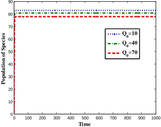
Figures have been plotted between dependent variables and time for different parameter values to shows changes occurring in population with time under different conditions. The results of numerical simulation are displayed graphically. In figure (1) the
x
,
T
1 andT
2 are plotted against time. From figure it is noted for given initial values the populations tend to their corresponding value of equilibrium pointP
*
and hence exists in the form of steady state assuring local stability ofP
*
. Figure shows that increasing the value of harvesting effort the population of species decreases and tends to zero ifE
≥
4
.
74
. Figure 3 and Figure 4 show that affect of primary and secondary toxicant on the population of species. From figures we can see that increasing the emittion rates of primary toxicant and secondary toxicant the population of species decreases. It can also be checked that all inequalities given by eq. (10) are satisfied for above equilibrium points and chosen parameters, so our system is stable for all values of delay, if it is stable in the absence of delay refer Figure 5.0 100 200 300 400 500 600 700 800 900 1000 0
10 20 30 40 50 60 70 80 90
Time
T
ot
al
P
op
u
lat
ion
x T
1
T
2
Figure-1: Stable behavior of
x
,
T
1 andT
2with time and other parameter values are same as (a).0 100 200 300 400 500 600 700 800 900 1000 -20
0 20 40 60 80 100 120
Time
P
o
pul
a
ti
o
n o
f Spe
c
ie
s
E=0 E=1 E=3 E=4.74
0 100 200 300 400 500 600 700 800 900 1000 0
10 20 30 40 50 60 70 80 90
Time
P
o
pul
a
ti
o
n o
f Spe
c
ie
s Q
0=10
Q
0=40
Q0=70
Figure-3. Variation of the population of species with time for different values of
Q
0and other parameter values are same as (a).0 100 200 300 400 500 600 700 800 900 1000 82
84 86 88 90 92 94 96 98 100
Time
P
o
pul
a
ti
o
n o
f Spe
c
ie
s
θ=0.01
θ=1
θ=4
Figure-4: Variation of the population of species with time for different values of
θ
and other parameter values are same as (a).0 10 20 30 40 50 60 70 80 90
0 2 4 6 8 10 12 14 16
Population of Species
C
on
c
e
n
tr
at
ion
of
P
r
im
ar
y T
oxi
c
an
t
Equilibrium Point
0 10 20 30 40 50 60 70 80 90
0 2 4 6 8 10 12 14 16
Population of Species
C
on
c
e
n
tr
at
ion
of
P
r
im
ar
y T
oxi
c
an
t
Equilibrium Point
Figure-5a. Figure-5b.
Figure 5: Graph of population of species verses concentration of primary toxicant for different values of delay.
20
=
7. DISCUSSION
In the present paper, we have discussed non–selective harvesting of a fishery resource that is affected by toxicant. We have structured toxicant into two levels according to its intensity – Primary toxicant that is of low intensity and secondary toxicant is highly toxic. It is assumed that growth rate coefficient and carrying capacity of logistically growing fish species are adversely affected by presence of toxicant and decreases with increase in toxicant level. The primary toxicant gets transformed into secondary toxicant after a constant time lag
τ
.We have proved positivity and boundedness of solution of system. Using stability theory of differential equation, we have also proved the existence of interior equilibrium and discussed stability of the system under certain conditions and found the condition for persistence of the system.It has been observed that increase in toxicant above certain level leads to extinction of species. We obtained the conditions under which system is stable for
τ
=
0
and also obtained criteria for no stability change whenτ
≠
0
. A least critical value of delay is also obtained at which stability change occur.An optimal policy to harvest fish population is discussed by using Pontryagin’s Maximum principle, optimal levels of harvesting effort, fish population and toxicants are obtained. It has been noted that increase in toxicant concentration decreases the optimal levels of harvesting effort and fish population. It has also been observed that sufficiently large value of discount rate decreases the net economic revenue to the society.
ACKNOWLEDGEMENT
Second author Dr. Rachana Pathak thankfully acknowledges the NBHM (2/40(29)/2014/R&D-11/14138) for the financial assistance in the form of PDF.
REFERENCES
1. H.I. Freedman and J.B. Shukla, Models for the effect of toxicant in single species and predator–prey systems, J.Math. Biol., 30(1991), 15–30.
2. T.G. Hallam and C.E. Clark, Nonautonomous logistic equations as models of population in a deteriorating environment, J. Theor. Biol., 93(1982), 303–311.
3. T.G. Hallam, C.E. Clark and G.S. Jordan, Effects of toxicants on populations: a qualitative approach II, First Order Kinetics, J. Math. Biol. 18(1983), 25–37.
4. T.G. Hallam, C.E. Clark and R.R. Lassiter, Effects of toxicants on populations: a qualitative approach I, Equilibrium Environmental Exposure, Ecol. Model. 18(1983), 291–304.
5. T.G. Hallam and J.T. De Luna, Effects of toxicants on populations: a qualitative approach III, Environmental and food chain pathways, J. Ther. Biol. 109(1984), 411–429.
6. J.B. Shukla, A.K. Agarwal, P. Sinha, and B.Dubey, Modelling effects of primary and secondary toxicants on renewable resources, Natural Resource Modelling, Spring16(1)(2003), 99–120.
7. M. Agarwal and S. Devi, A Resource-Dependent Competition Model: Effects of Toxicants Emitted from External Sources as well as formed by Precursors of Competing Species, Nonlinear Analysis: Real World Applications, 12(2011), 751-766.
8. M. Agarwal and R. Pathak, Persistence and Optimal Harvesting of Prey-Predator Model with Holling Type III Functional Response,International Journal of Engineering, Science and Technology, 4(3)(2012),78-96. 9. M. Agarwal and R. Pathak, Stability and Hopf Bifurcation Analysis in Ecological System with Two Delays,
International Journal of Engineering, Science and Technology, 3(8) (2011), 41-53.
10. G.Butler, H.I. Freedom and P.Waltman. Uniformly Persistent systems. Proc. Am. Math. Soc., 96(1986), 425-430.
BIOGRAPHICAL NOTES
Manju Agarwal holds Ph.D. Degree in Applied Mathematics and currently she is working as a Professor and Former Head of Department of Mathematics and Astronomy, Lucknow University, Lucknow. Her areas of research interest are Mathematical Modeling, Environmental Pollution and Mathematical Ecology.
Pragya Mishra holds Ph.D. Degree in Applied Mathematics and currently she is working as a Assistant Professor in Govt. P.G. College, Hardoi. Her areas of research interest are Mathematical Modeling and Environmental Pollution. Rachana Pathak holds Ph.D. Degree in Applied Mathematics and currently she is doing PDF in Lucknow University, Lucknow. Her areas of research interest are Mathematical Modeling and Mathematical Ecology.
Source of support: Nil, Conflict of interest: None Declared