Volume 2014, Article ID ama0114, 11 pages ISSN 2307-7743
http://scienceasia.asia
SOLUTION OF THIRTEENTH ORDER BOUNDARY VALUE PROBLEMS BY DIFFERENTIAL TRANSFORMATION METHOD
MUZAMMAL IFTIKHAR, HAMOOD UR REHMAN, AND MUHAMMAD YOUNIS
Abstract. The aim of this paper is to use the differential transformation method (DTM), a semi-numerical and semi-analytic technique for solving lin-ear and nonlinlin-ear thirteenth order boundary value problems. The approximate solution of the problem is calculated in terms of a rapidly convergent series. Two numerical examples have been considered to illustrate the efficiency and implementation of the method and the results are compared with the method developed in [1].
1. Introduction
Higher order boundary value problems occure in the study of fluid dynamics, astrophysics, hydrodynamic, hydro magnetic stability, astronomy, beam and long wave theory, induction motors, engineering and applied physics. The boundary value problems of higher order have been examined due to their mathematical im-portance and applications in diversified applied sciences.
The theory of differential transformation was established by Zhou [10]. The au-thor solved linear and non-linear IVPs arising in circuit analysis. Pukhov [4] also studied differential transformation method at the same time. The method con-structs an analytical solution for differential equations in the form of a series. It is a semi-numerical and semi-analytic technique that formulizes the Taylor series in a totally different manner. It differs from the traditional higher order Taylor se-ries method, which computationally, takes more time for higher orders BVPs. The DTM transforms the given BVP into a recurrence relation that finally leads to the solution of a system of algebraic equations as coefficients of a power series solution. The method is useful to obtain both exact and approximate solutions of linear and non-linear BVPs. There is no need to discretization, linearization or perturbation, large computational work and round-off errors are avoided.
Siddiqi and Iftikhar used the variation of parameter method for solving the seventh-order boundary value problems in [7]. Siddiqi and Akram [5] used nonic spline and non-polynomial spline technique for the numerical solution of eighth-order lin-ear special case boundary value problems. These methods have also been proven to be second order convergent. Recently, Akram and Rehman presented the nu-merical solution of eighth-order boundary value problems using the reproducing kernel space method [2]. Geng and Li [3] construct a reproducing kernel space and solve a class of linear tenth-order boundary value problems using reproducing
2010Mathematics Subject Classification. 34B05; 34B15.
Key words and phrases. Approximate solution; Differential transformation method; Thirteenth order boundary value problems; Linear and nonlinear problems; Series solution.
c
kernel method. Siddiqiet al.[6] used the variational iteration technique for the so-lution of tenth order boundary value problem. Siddiqi and Akram [8] presented the numerical solutions of the tenth-order linear special case boundary value problems using eleventh degree spline. Siddiqi and Iftikhar [9] determined the approximate solutions of seventh, eighth, and tenth-order boundary value problems using homo-topy analysis method (HAM). Adeosunet al.[1] presented the variational iteration method (VIM) to find the approximate solutions of linear and nonlinear thirteenth order boundary value problems
In the present paper, thirteenth-order boundary value problems are solved using DTM. The following thirteenth-order boundary value problems are considered
u(13)(x) = f(x, u(x)), a≤x≤b, u(i)(a) = A
i, u(j)(b) = B
j
(1. 1)
where fori= 0,1,2, ...,6 andj = 0,1, ...,5. Ai’s and Bj’s are finite real constants. Alsof(x, u(x)) is a continuous function on [a, b].
In the following section the differential transformation method is discussed.
2. Differential Transformation Method
The differential transformation of thekth derivative of a functionf(x), atx=x0, is defined as
F(k) = 1
k! [
dkf(x) dxk
]
x=x0 (2. 1)
and the inverse differential transformation ofF(k) is defined by
f(x) =
∞
∑
k=0
F(k)(x−x0)k. (2. 2)
In real applications, the functionf(x) can be expressed as a finite series and Eq. ( 2. 2 ) can be written as
f(x) = N ∑
k=0
F(k)(x−x0)k. (2. 3)
SubstitutingF(k) from Eq. ( 2. 1 ) into Eq. ( 2. 2 ), gives
(2. 4) f(x) =
∞
∑
k=0
(x−x0)k 1
k! [
dkf(x) dxk
]
x=x0
,
which is the Taylor series forf(x) at x=x0. From Eq. ( 2. 1 ) and Eq. ( 2. 2 ), the following theorems can be proved.
Proof Using the definition ( 2. 1 ), yields
G(k) = 1
k! [
dkg(x)
dxk ]
x=0
,
(2. 5)
H(k) = 1
k! [
dkh(x) dxk
]
x=0
,
(2. 6)
F(k) = 1
k! [
dk
dxk[g(x) +h(x)] ]
x=0
.
(2. 7)
Using Eqs. ( 2. 5 ) - ( 2. 7 ), yield
F(k) = G(k) +H(k).
(2. 8)
Similarly, it can be proved that
F(k) = G(k)−H(k).
(2. 9)
Theorem 2Iff(x) =cg(x), thenF(k) =cG(k), wherecis a constant. Proof Using the definition ( 2. 5 ),
G(k) = 1
k! [
dkg(x) dxk
]
x=0
,
(2. 10)
F(k) = 1
k! [
dk dxk[cg(x)]
]
x=0 = c1
k! [
dkg(x) dxk
]
x=0
.
(2. 11)
Using Eqs. ( 2. 10 ) and ( 2. 11 ), give
F(k) =cG(k).
(2. 12)
Theorem 3Iff(x) =dmdxgm(x), thenF(k) = (k+m)G(k+m). Proof By definition ( 2. 5 ),
F(k) = 1
k! [
dk dxk
[
dmg(x)
dxm ]]
x=0 = (k+ 1)(k+ 2)· · ·(k+m)
(k+m)!
[
dk+mg(x) dxk+m
]
x=0
,
(2. 13)
then
F(k) = (k+m)!
Theorem 4Iff(x) =g(x)h(x), thenF(k) =∑kk
1=0G(k1)H(k−k1).
Proof By definition ( 2. 5 ),
F(0) = 1
0![g(x)h(x)]x=0=G(0)H(0), (2. 15)
F(1) = 1 1!
[
d
dx[g(x)h(x)]
]
x=0 =
[
dg(x)
dx h(x) +g(x) dh(x)
dx
]
x=0 = G(1)H(0) +G(0)H(1),
(2. 16)
F(2) = 1 2!
[
d2
dx2[g(x)h(x)] ]
x=0
= G(2)H(0) +G(1)H(1) +G(0)H(2).
(2. 17)
In general, it can be written as
F(k) = k ∑
k2=0 k2 ∑
k1=0
G(k1)H(k2−k1)L(k−k2). (2. 18)
Theorem 5Iff(x) =eλx, thenF(k) = λkk!. Proof Using definition ( 2. 5 ), gives
F(k) = 1
k! [
dk dxke
λx ]
x=0
= λ
k
k!. (2. 19)
Theorem 6(i) Iff(x) =Sin(αx+β), thenF(k) =αkk!Sin(kπ2 +β). (ii) Iff(x) =Cos(αx+β), thenF(k) = αk
k!Cos (kπ
2 +β )
.
Proof (i) Using definition ( 2. 5 ), gives
F(k) = 1
k! [
dk
dxkSin(αx+β) ]
x=0
= α
k
k!Sin (
kπ
2 +β )
.
(2. 20)
(ii) Using definition ( 2. 5 ), gives
F(k) = 1
k! [
dk
dxkCos(αx+β) ]
x=0
= α
k
k!Cos (
kπ
2 +β )
.
(2. 21)
Theorem 7Iff(x) =g(x)h(x)l(x), then
F(k) =∑kk 2=0
∑k2
Proof By definition ( 2. 5 ),
F(0) = 1
0![g(x)h(x)l(x)]x=0=G(0)H(0)L(0), (2. 22)
F(1) = 1 1!
[
d
dx[g(x)h(x)l(x)]
]
x=0 =
[
dg(x)
dx h(x)l(x) +g(x) dh(x)
dx l(x) +g(x)h(x) dl(x)
dx
]
x=0 = G(1)H(0)L(0) +G(0)H(1)L(0) +G(0)H(0)L(1),
(2. 23)
F(2) = 1 2!
[
d2
dx2[g(x)h(x)l(x)] ]
x=0
= G(2)H(0)L(0) +G(1)H(1)L(0) +G(1)H(0)L(1)
+G(1)H(1)L(0) +G(0)H(2)L(0) +G(0)H(1)L(1)
+G(1)H(0)L(1) +G(0)H(1)L(1) +G(0)H(0)L(2).
(2. 24)
In general, it can be written as
F(k) = k ∑
k2=0 k2 ∑
k1=0
G(k1)H(k2−k1)L(k−k2). (2. 25)
2.1. Analysis of the Method. The followingnth order BVP is considered
u(n)=f(x, u, u′, u′′,· · ·, u(n−1)), a≤x≤b,
(2. 26)
with the boundary conditions
B
(
u,du dx,
d2u
dx2,· · ·,
d(n−1)u
dx(n−1) )
.
(2. 27)
The differential transformation of the problem ( 2. 26 ) is
U(k+n) = F(k) (k+n)!, (2. 28)
whereF(k) is the differential transformation off(x, u, u′, u′′,· · ·, u(n−1)). The transformed boundary conditions can be written as
U(k) =A, U(m) = N ∑
k=0 m∏−1
i=1
(k−i)U(k) =Bm, (m < n), (2. 29)
wherem is the order of the derivative in the boundary conditions andA, Bm are real constants.
Using Eqs. ( 2. 28 ) and ( 2. 29 ), the values of U(i), i = 1,2,3,· · · can be determined and then using the inverse differential transformation, the following approximate solution uptoO(xN+1) can be determined
e
u= N ∑
k=0
xkU(k).
(2. 30)
3. Numerical Examples
Example 3.1The linear thirteenth order BVP, is considered as
u(13)(x) = Cosx−Sinx, 0≤x≤1,
(3. 1)
subject to the boundary conditions
u(0) = 1, u(1) =Cos(1) +Sin(1), u(1)(0) = 1, u(1)(1) =Cos(1)−Sin(1),
u(2)(0) = −1, u(2)(1) =−Sin(1)−Cos(1),
u(3)(0) = −1, u(3)(1) =−Cos(1) +Sin(1), u(4)(0) = 1, u(4)(1) =Cos(1) +Sin(1),
u(5)(0) = 1, u(5)(1) =Cos(1)−Sin(1).
u(6)(0) = −1,
(3. 2)
The exact solution of the problem isu(x) =Cosx+Sinx.
Applying the theorems 1, 3 and 6 the differential transformation of the problem ( 3. 1 ) can be determined as
U(k+ 13) = k! (k+ 13)!
[ 1
k!Cos (
πk
2 )
− 1 k!Sin
(
πk
2 )]
.
(3. 3)
Using the Eq. ( 2. 1 ), the boundary conditions ( 3. 2 ) at x0 = 0, can be transformed as
U(0) = 1, U(1) = 1, U(2) = −2!1,
U(3) = −3!1, U(4) = 4!1, U(5) = 5!1, U(6) = −6!1,
} (3. 4)
∑n
k=0U(k) =Cos(1) +Sin(1), ∑n
k=0kU(k) =Cos(1)−Sin(1), ∑n
k=0k(k−1)U(k) =−Sin(1)−Cos(1), ∑n
k=0k(k−1)(k−2)U(k) =−Cos(1) +Sin(1), ∑n
k=0k(k−1)(k−2)(k−3)U(k) =Cos(1) +Sin(1), ∑n
k=0k(k−1)(k−2)(k−3)(k−4)U(k) =Cos(1)−Sin(1), (3. 5)
where n is a sufficiently large integer. Using the recurrence relation ( 3. 3 ), the transformed boundary conditions ( 3. 4 ) and the inverse differential transformation ( 2. 3 ), the following series solution forn= 13, can be written
u(x) = 1 +x−x
2 2 −
x3
6 +
x4
24+
x5
120−
x6
720 +Ax
7+Bx8+Cx9
+Dx10+Ex11+F x12+ x 13
6227020800+O(x 14), (3. 6)
where, according to the definition ( 2. 1 )
A= u(7)7!(0) =U(7), B= u(8)8!(0) =U(8), C= u(9)9!(0) =U(9), D=u(10)10!(0) =U(10), E= u(11)11!(0) =U(11), F =u(12)12!(0) =U(12).
From the transformed boundary conditions ( 3. 5 ), the following system of linear equations in terms ofA,B, C,D,E andF can be determined
8605396801
6227020800+A+B+C+D+E+F=Cos[1] +Sin[1],
−143700479
479001600 + 7A+ 8B+ 9C+ 10D+ 11E+ 12F =Cos[1]−Sin[1],
−54885599
39916800+ 42A+ 56B+ 72C+ 90D+ 110E+ 132F =−Cos[1]−Sin[1], 1209601
3628800+ 210A+ 336B+ 504C1 + 720D1 + 990F+ 1320G=−Cos[1] +Sin[1], 544321
362880+ 840A+ 1680B+ 3024C1 + 5040D1 + 7920F+ 11880G=Cos[1] +Sin[1], 1
40320+ 2520A+ 6720B+ 15120C1 + 30240D1 + 55440F+ 95040G=Cos[1]−Sin[1]. The solution of the above system, yields
A=−0.00019841261645169112, B = 0.00002480111056133196, C= 2.7568717766803008×10⁻⁶, D=−2.769904021536794×10⁻⁷,
E=−2.4115063057288555×10⁻⁸, F = 1.8105803100768588×10⁻⁹. The series solution can, thus, be written as
u(x) = 1 +x−x
2 2 −
x3 6 +
x4 24+
x5 120−
x6
720 −0.000198413x
7+ 0.0000248011x8
+2.75687×10−6x9−2.7699×10−7x10−2.41151×10−8x11+ 1.81058×10−9x12
+ x
13
6227020800+O(x 14). (3. 8)
0.2 0.4 0.6 0.8 1 1.1
1.2 1.3 1.4
Figure 1. Comparison of the approximate solution with the exact solution for problem 3.1. Dotted line: approximate solution, solid line: the exact solution.
0.2 0.4 0.6 0.8 1
2·10-15 4·10-15 6·10-15 8·10-15 1·10-14 1.2·10-14
Figure 2. Absolute errors for problem 3.1.
Example 3.2The thirteenth order non-linear BVP is considered as
u(13)(x) = e−xu2(x), 0≤x≤1,
(3. 9)
subject to the boundary conditions
u(0) = 1, u(1) =e, u(1)(0) = 1, u(1)(1) =e,
u(2)(0) = 1, u(2)(1) =e, u(3)(0) = 1, u(3)(1) =e,
u(4)(0) = 1, u(4)(1) =e,
u(5)(0) = 1, u(5)(1) =e. u(6)(0) = 1,
(3. 10)
The exact solution of the problem isv(x) =ex.
Applying the theorems (1-7), the differential transformation of the problem ( 3. 9 ) can be determined as
U(k+ 13) =− k! (k+ 13)!
k ∑
k2=0 k2 ∑
k1=0
(−1)k1U(k−k
2)U(k2−k1)
k1!
.
(3. 11)
Using Eq. ( 2. 1 ), the boundary conditions ( 3. 10 ) atx0= 0, can be transformed as
U(0) = 1, U(1) = 1, U(2) = 2!1,
U(3) = 3!1, U(4) = 4!1, U(5) = 5!1, U(6) = 6!1,
} (3. 12)
∑n
k=0U(k) =e, ∑n
k=0kU(k) =e, ∑n
k=0k(k−1)U(k) =e, ∑n
k=0k(k−1)(k−2)U(k) =e, ∑n
k=0k(k−1)(k−2)(k−3)U(k) =e, ∑n
where nis a sufficiently large integer. Using the recurrence relation ( 3. 11 ), the transformed boundary conditions ( 3. 12 ) and the inverse differential transforma-tion ( 2. 3 ), the following series solutransforma-tion uptoO(x14) can be determined
u(x) = 1 +x+x 2 2 +
x3 6 +
x4 24+
x5 120+
x6 720 +Ax
7+Bx8+Cx9
+Dx10+Ex11+F x12+ x 13
6227020800+O(x 14), (3. 14)
where, according to the definition ( 2. 1 )
A= u(7)7!(0) =U(7), B= u(8)8!(0) =U(8), C= u(9)9!(0) =U(9), D=u(10)10!(0) =U(10), E= u(11)11!(0) =U(11), F =u(12)12!(0) =U(12).
} (3. 15)
From the transformed boundary conditions ( 3. 13 ), the following system of linear equations in terms ofA,B andC can be determined
16925388481
6227020800 +A+B+C+D+E+F=e, 1301287681
479001600 + 7A+ 8B+ 9C+ 10D+ 11E+ 12F =e, 108108001
39916800 + 42A+ 56B+ 72C+ 90D+ 110E+ 132F =e, 9676801
3628800+ 210A+ 336B+ 504C1 + 720D1 + 990F+ 1320G=e, 907201
362880+ 840A+ 1680B+ 3024C1 + 5040D1 + 7920F+ 11880G=e, 0641
40320+ 2520A+ 6720B+ 15120C1 + 30240D1 + 55440F+ 95040G=e. (3. 16)
The solution of the above system, yields
A= 0.00019841261021669805, B= 0.000024802098855594142, C= 2.75451301223356×10⁻⁶, D= 2.7708206549274656×10⁻⁷,
E= 2.4060411409761992×10⁻⁸, F = 2.3783375635762833×10⁻⁹. The series solution can, thus, be written as
u(x) = 1 +x+x 2 2 +
x3 6 +
x4 24+
x5 120+
x6
720+ 0.000198413x
7+ 0.0000248021x8
+2.75451×10−6x9+ 2.77082×10−7x10+ 2.40604×10−8x11
+2.37834×10−9x12+ x 13
6227020800+O(x 14). (3. 17)
0.2 0.4 0.6 0.8 1 1.25
1.5 1.75 2 2.25 2.5 2.75
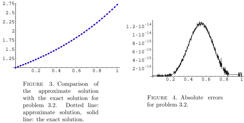
Figure 3. Comparison of the approximate solution with the exact solution for problem 3.2. Dotted line: approximate solution, solid line: the exact solution.
0.2 0.4 0.6 0.8 1
2·10-15 4·10-15 6·10-15 8·10-15 1·10-14 1.2·10-14
Figure 4. Absolute errors for problem 3.2.
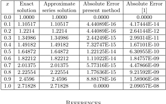
Conclusion In this paper, the differential transformation method has been applied to obtain the numerical solution of linear and nonlinear thirteenth order boundary value problems. The present method has been applied in a direct way without using linearization, discretization, or perturbation. By increasing the order of approximation more accuracy can be obtained. Comparison of the numerical results with the existing technique [1] shows that the present method is more accurate.
Table 1. Comparison of numerical results for Example 3.1
x Exact Approximate Absolute Error Absolute Error solution series solution present method [1]
0.0 1.0000 1.0000 0.0000 0.0000
Table 2. Comparison of numerical results for Example 3.2
x Exact Approximate Absolute Error Absolute Error solution series solution present method [1]
0.0 1.0000 1.0000 0.0000 0.0000
0.1 1.10517 1.10517 4.44089E-16 4.17444E-14 0.2 1.2214 1.2214 4.44089E-16 2.64144E-12 0.3 1.34986 1.34986 2.44249E-15 2.99314E-11 0.4 1.49182 1.49182 7.32747E-15 1.67101E-10 0.5 1.64872 1.64872 1.22125E-14 6.30955E-10 0.6 1.82212 1.82212 1.11022E-14 1.84757E-09 0.7 2.01375 2.01375 5.77316E-15 4.47866E-09 0.8 2.22554 2.22554 1.77636E-15 9.21592E-09 0.9 2.4596 2.4596 8.88178E-16 1.58906E-08 1.0 2.71828 2.71828 0.0000 2.09057E-08
References
[1] T. A. Adeosun, O. J. Fenuga, S. O. Adelana, A. M. John, O. Olalekan, and K. B. Alao, Vari-ational iteration method solutions for certain thirteenth order ordinary differential equations, Appl. Math.4(2013), 1405–1411.
[2] G. Akram and H. U. Rehman, Numerical solution of eighth order boundary value problems in reproducing kernel space, Numer. Algor.62(3)(2013), 527–540.
[3] F. Geng and X. Li, Variational iteration method for solving tenth-order boundary value problems, Math. Sci.3(2)(2009), 161–172.
[4] G. E. Pukhov,Differential transformations and mathematical modelling of physical processes, Naukova Dumka, Kiev, Ukraine (1986).
[5] S. S. Siddiqi and G. Akram, Solution of eighth-order boundary value problems using the non-polynomial spline technique, Intl. J. Comput. Math.84, No. 3(2007), 347–368. [6] S. S. Siddiqi, G. Akram, and S. Zaheer, Solution of tenth order boundary value problems
using variational iteration technique, Eur. J. Sci. Res.30(3)(2009), 326–347.
[7] S. S. Siddiqi and M. Iftikhar,Solution of seventh order boundary value problems by variation of parameters method, Res. J. Appl. Sci., Engin. Tech.5(1)(2013), 176–179.
[8] Shahid S. Siddiqi and Ghazala Akram, Solutions of tenth-order boundary value problems using eleventh degree spline, Appl. Math. Comput.185(2007), 115–127.
[9] S. S. Siddqi and M. Iftikhar, Numerical solution of higher order boundary value problems, Abstract Appl. Anal.2013(2013), Article ID 427521, 12 pages, doi:10.1155/2013/427521. [10] J. K. Zhou,Differential transformation and its applications for electrical circuits, Huazhong
University Press, Wuhan, China (1986).
Department of Mathematics, University of Education, Okara Campus, Okara 56300, Pakistan
Department of Mathematics, University of Education, Okara Campus, Okara 56300, Pakistan