3D Modelling With Linear Approaches Using Geometric Primitives

31

3D MODELLING WITH LINEAR APPROACHES

USING GEOMETRIC PRIMITIVES

Mochammad Zuliansyah

Informatics Engineering, Faculty of Engineering, ARS International University, Bandung 40282, Indonesia

E-mail: [email protected]

Abstract

In this paper, we study linear approaches for 3D model acquisition from non-calibrated images. First, the intrinsic and extrinsic camera calibration is taken into consideration. In particular, we study the use of a specific calibration primitive: the parallelepiped. Parallelepipeds are frequently present in man-made environments and naturally encode the affine structure of the scene. Any information about their euclidean structure (angles or ratios of edge lengths), possibly combined with information about camera parameters is useful to obtain the euclidean reconstruction. We propose an elegant formalism to incorporate such information, in which camera parameters are dual to parallelepiped parameters, i.e. any knowledge about one entity provides constraints on the parameters of the others. Consequently, an image a parallelepiped with known Euclidean structure allows to compute the intrinsic camera parameters, and reciprocally, a calibrated image of a parallelepiped allows to recover its euclidean shape (up to size). On the conceptual level, this duality can be seen as an alternative way to understand camera calibration: usually, calibration is considered to be equivalent to localizing the absolute conic or quadric in an image, whereas here we show that other primitives, such as canonic parallelepipeds, can be used as well. While the main contributions of this work concern the estimation of camera and parallelepiped parameters. The complete system allows both calibration and 3D model acquisition from a small number of arbitrary images with a reasonable amount of user interaction.

Keywords: parallelepiped, the affine structure, euclidean structure, 3D model

1.

Introduction

The camera and parallelepiped parameters are recovered in two steps. First, their intrinsic and orientation parameters are computed. The original approach for this step was introduced in Wilczkowiak et al. [1] and consists on parameterization of the intrinsic matrices of all the objects (cameras and parallelepipeds) in terms of the intrinsic matrix of a reference object. The algorithm proposed later Wilczkowiak et al. [2] exploits the fact that the parallelepipeds projection matrices can be factorized into two parts, representing respectively camera and parallelepiped parameters and allows to treat the available data simultaneously without privileging any primitive.

Our calibration approach is conceptually close to self-calibration methods, especially those that upgrade affine to euclidean structure [3,4] or those that consider special camera motions [5-7]. The way metric information on a parallelepiped is used is also similar to vanishing point based methods [8-11]. Some properties of our algorithm are also common with plane-based approaches [12-17]. While more flexible than standard calibration

techniques, plane-based approaches still require either euclidean information or, for self-calibration, many images in general position [18]. In this sense, our approach is a generalization of plane-based methods with metric information to three-dimensional parallelepipedic patterns. This allows to handle missing data and unknown scale factors and simplifies the formulation of calibration constraints. Finally, our approach can be compared to methods using complex primitives for the scene representation. However, unlike most methods of this type, we use the parallelepiped parameters directly to solve the calibration problem without requiring non-linear optimization methods.

A parallelepiped encodes naturally the affine properties of the scene and facilitates modeling the remaining metric part. The representation of a parallelepiped given below is based on the formalism proposed in Wilczkowiak et al. [1,19]. A parallelepiped is defined by twelve parameters: six extrinsic parameters describing its orientation and position, and six intrinsic parameters describing its metric shape: three dimension parameters (edge lengths l1; l2 and l3) and three angles between edges (µ12; µ23; µ13). The parallelepiped may be represented compactly in matrix form by a 4 x 4 matrix N: ~ 1 L O v S

N _{T ⎟⎟}

⎠ ⎞ ⎜⎜ ⎝ ⎛ = (1) where S is a rotation matrix and v a vector, representing the parallelepiped's pose (extrinsic parameters). The 4 x 4 matrix ~L represents the parallelepiped's shape:

( ) ⎟ ⎟ ⎟ ⎟ ⎟ ⎟ ⎟ ⎠ ⎞ ⎜ ⎜ ⎜ ⎜ ⎜ ⎜ ⎜ ⎝ ⎛ − − − − = 1 0 0 0 0 3 0 0 0 0 0 2 12 2 12 13 23 2 12 2 13 2 12 12 12 13 23 3 12 2 13 3 12 2 1 ~ s c c c s c s l s c c c l s l c l c l l L (2)

With: cij =cos

θ

θ

θ

] [

π

The matrix ~L represents the affine transformation between a canonical cube and a parallelepiped with the given shape. Formally, a vertex (±1; ±1; ±1; 1)T of the canonical cube is mapped, by ~L, to a vertex of our parallelepiped's intrinsic shape. Then, the pose part of N maps the vertices into the world coordinate system. Other parameterizations for ~L may be chosen, but the above one is attractive due to its upper triangular form. This underlines the fact that ~L plays the same role for the parallelepiped as the calibration matrix K for a camera. The analogous entity to a camera's Image of the Absolute Conic(IAC) ω, is the matrix µ, defined by:

⎟ ⎟ ⎟ ⎠ ⎞ ⎜ ⎜ ⎜ ⎝ ⎛ 2 3 23 3 2 13 3 1 23 3 2 2 2 12 2 1 13 3 1 12 2 1 2 1 cos cos cos cos cos cos ~ ~ l l l l l l l l l l l l l l l L LT θ θ θ θ θ θ µ (3) where L is the upper left 3 x 3 matrix of ~L.

Hence, there is a seemingly perfect symmetry between intrinsic parameters of cameras and parallelepipeds. The only difference is that in some cases, the size of a parallelepiped matters, as will be explained below. As for cameras, the fact that K33 = 1 allows us to fix the scale factor in the relation ω ∞ K-TK-1, and thus to extract K uniquely from the IAC ω, e.g. using Cholesky decomposition. As for parallelepipeds, however, we have no such constraint on its “calibration matrix" L, so the relation µ ∞ LTL gives us a parallelepiped's Euclidean shape, but not its (absolute) size. This does

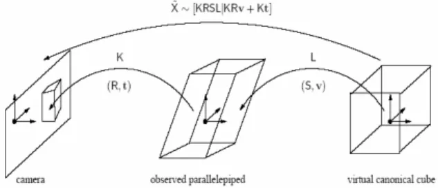
Figure 1. The projection of the canonic parallelepiped (cube) into the image. Matrices K, L correspond to intrinsic parameters of camera and parallelepiped and (R; t),(S; v) correspond to extrinsic parameters of camera and parallelepiped, respectively.

not matter in general, since we are usually only interested in reconstructing a scene up to some scale. However, when reconstructing several parallelepipeds, one needs to recover at least their relative sizes.

There are many possibilities of defining the size of parallelepipeds. We choose the following definition, due to its appropriateness in the equations underlying our calibration and reconstruction algorithms below: the size of a parallelepiped is defined as

s = (det L)1/3 (4)

This definition is actually directly linked to the parallelepiped's volume: s3 = det L = Vol=8 (the factor 8 arises since our canonic cube has an edge length of 2).

2.

Methods

Using parallelepipeds as natural calibration objects offers several advantages over standard self-calibration approaches. Firstly, fewer correspondences are needed; five and a half points extracted per image are sufficient, and even fewer inter-image correspondences are needed. Secondly, the reduced canonical parallelepiped projection matrices encode the affine properties of the scene. In consequence, the calibration problem is reduced to a self-calibration problem where the plane at infinity is already localized [3,4] or where the cameras are stationary [5-7].

The calibration algorithm described in this section is based on the parameterization of the intrinsic matrices of all the objects in terms of the intrinsic matrix of a reference primitive. This is done using parallelepiped projection matrices. Due to the necessity of choice of reference object the properties of this algorithm are less interesting than properties of the factorization algorithm given in the following section.

well as parallelepipeds and the edges are the projections. We assume that the graph is connected and, consequently, for each object i the transformation Gi such that GiT µ0Gi can be computed. When this is not a case, all the connected parts of the graph have to be calibrated separately. Our calibration approach consists of two stages. First, all the available linear equations are used to determine µ0 (the system is solved using SVD). If there is a unique solution, then we are done (from µ0, all the camera and parallelepiped intrinsics can be computed using the Gik). The decision if the system is under-constrained may be taken on the basis of a singular value analysis. This also gives the degree of the ambiguity (dimension of the solution space). In practice, this is usually two or lower. Hence, two quadratic equations are in general suffcient to obtain a finite number of solutions. Once the matrices ωi and µk are estimated, the matrices Ki and Li can be computed via Cholesky decomposition.

Finally, we propose the following algorithm:

1. Construct the graph with cameras and parallelepipeds as nodes and projections as edges, 2. Estimate the canonical projection matrices ~_Xik,

3. Choose a reference parallelepiped represented by µ0

4. Compute paths (shortest for example) connecting all the cameras i and parallelepipeds k to µ0 and use

them to compute transformations Gi, Gk,

5. Establish linear equation system on µ0 based on

prior knowledge of intrinsic parameters of cameras and parallelepipeds,

6. Solve the system to least squares,

7. If necessary, use the non-linear equations to resolve the remaining ambiguities on µ0,

8. Compute the matrices ωi , µk using µ0 and

transformations Gi, Gk

9. Extract the Ki, Lk from the ωi and the µk using e.g.

QR-decomposition. Note that at this stage the Lk

can only be recovered up to scale, i.e. the parallelepiped’s (relative) sizes remain undetermined,

10. Compute rotation matrices by factorization of a measurement matrix composed of matrices X’

ik.

The measurement matrix X contains all information that can be recovered from the parallelepipeds' image points alone. Since the measurement matrix is the product of a “motion matrix" ~M of 4 columns, with a “shape matrix" ~S of 4 rows, its rank can be 4 at most (in the absence of noise).

3.

Result and Discussion

The calibration approach presented before is well adapted to interactive 3D modeling from a few images. It has a major advantage over other methods: simplicity. Indeed, only a small amount of user interaction is

needed for both calibration and reconstruction: a few points must be picked in the image to define the primitives image positions.

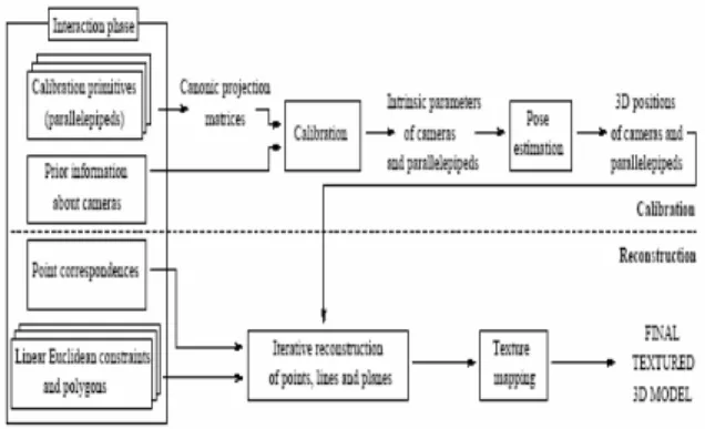
To reconstruct scene elements not belonging to the parallelepiped, constrained by bilinear relations such as collinearity, coplanarity or parallelism, we have implemented a multi-linear reconstruction method, introduced originally in Wilczkowiak et al. [2]. The reconstruction step is actually independent from the calibration method, although it uses the same input in the first step. Interestingly, it allows 3D models to be computed from non-overlapping photographs. The global scheme of our system is presented in Figure 2.

Figure 2. The calibration and reconstruction algorithms.

Finally, we propose the following reconstruction algorithm:

1: while !stop_condition do

2: for objects=points,lines+planes: do

3: N=

∑

=

n

i1nb_of _coordinates(objectr[i])

4: initialize an empty linear equation system A0xnXnx1=B0x1

5: compute the indexing function (bijection)

F:idx→(I,j);idx є [1..N], where idx is

the index in XNx1 of the j-th coordinate

of the i-th object.

6: for all constraint c[k]: do 7: compute

(

)

mk k

N

mk× , ×1 := ( [ ]. , [ ]. 8:

add equations to the system:

⎥ ⎦ ⎤ ⎢ ⎣ ⎡ = ⎥ ⎦ ⎤ ⎢ ⎣ ⎡

= k

k k

B B B A

A

A: :

9: end for

10: solve AX = B

11: for idx=1..N: do

12: if variable_computed(idx) then 13: set (i,j):=F(idx)

14: set objects[i].coords[j]:=X(idx) 15: end if

16: end for

17: end for

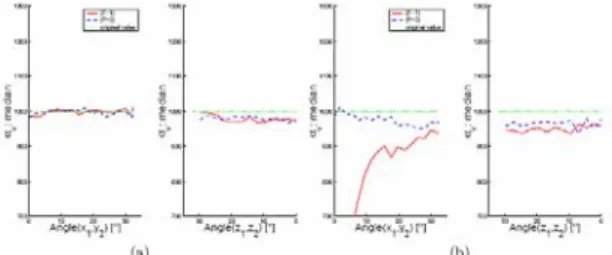
Let us study in more details the results of the intrinsic and extrinsic calibration. Let us first consider the behavior of our calibration method in a proximity of singular configurations (left and right extremities of Figures 3-5). It can be seen that at both initial and final positions P0 and Pn, calibration is very unstable, as expected. However, when the minimal angle between the camera axes is larger than 15° the method can be considered stable. All calibrations are successful (Figure 3a), the relative error on the obtained median values is not larger than 7% (Figure 4).As expected, calibration results obtained with the reference primitive method are less stable than those obtained with the factorization method. Indeed, as shown in Figure 4 the relative error on median values obtained with the reference primitive method is up to 9% (vs 7% for the factorization method). Also, reprojection error is more important (~1,5 pixel for 1 primitive and ~8 pixels for 2 primitive based calibration vs ~0,5 pixel and ~6 pixels for the factorization method). Naturally, calibration results are more stable using two parallelepipeds than with a single one. First, using larger number of primitives decreases the possibility for singulararity. Figure 5b shows results for the second camera for one and two parallelepiped based calibration using information on right parallelepiped angles. While a relative position between the first parallelepiped and second camera is singular for the calibration, adding a second parallelepiped stabilizes the configuration. In non-singular configurations the larger number of primitives and related increased number of equations result in more accurate calibration (Figures 3-5). However, introducing additional primitives increases the reprojection error (see Figure 3b). Comparing Figures 4 and 5 it can be seen that using the information about the right parallelepiped angles decreases importantly the number of singularities.

Figure 6 presents the results for the estimation of the camera's rotation and translation. Extrinsic calibration was performed only when the previous internal

Figure 3. (a) Number of successful calibrations; (b) Median values of reprojection errors. Plots described by (F-*) and (P-*) correspond, respectively, to factorization and reference primitive methods; plots described by (*-1) and (*-2) correspond to calibration based on 1 and 2 parallelepipeds.

Figure 4. Median values obtained for the focal length of (a) first camera; (b) second camera. Notations are similar to Figure 3.

Figure 5. Calibration results using the factorization method for the estimation of local length of (a) the 1st camera and (b) the second camera, using the known right parallelepipeds angles.

Figure 6. Extrinsic calibration results. (a) Median values of the rotation error; (b) Median values of the angle between the true and the estimated direction between the cameras-parallelepiped relative translation vectors. Notations are similar to Figure 3.

projections of at most 12 points per image (6 per parallelepiped projection). However, increasing the number of scene constraints (i.e. number of calibration primitives) increases also the reprojection error. The increase of the reprojection error for the methods based on two calibration parallelepipeds can be seen in chart 3b.

4. Conclusion

An image of parallelepiped with known Euclidean structure allows the intrinsic camera parameters computing, and reciprocally, a calibrated image of a parallelepiped allows its euclidean shape (up to size) recovering. On the conceptual level, this duality can be seen as an alternative way to understand camera calibration which is usually considered to be equivalent to localizing the absolute conic or quadric of an image, other primitives, such as canonic parallelepipeds, can be used as well. The complete system allows both calibration and 3D model acquisition from a small number of arbitrary images with a reasonable amount of user interaction.

References

[1] M. Wilczkowiak, E. Boyer, P. Sturm, In: A. Heyden, G. Sparr, M. Nielsen, P. Johansen (Eds.), Proceedings of the 7th European Conference on Computer Vision, Copenhagen, Denmark, 2002, p. 221.

[2] M. Wilczkowiak, P. Sturm, E. Boyer. Using Geometric Constraints Through Parallelepipeds for Calibration and 3D Modelling, Research Report 5055, inria, Grenoble, France, 2003.

[3] R.I. Hartley, Proceeding of the Darpa-espritworkshop on Applications of Invariants in Computer Vision, Azores, Portugal, 1993, p.187. [4] M. Pollefeys, L. van Gool, Proceedings of the

Conference on Computer Vision and Pattern Recognition, Puerto Rico, USA, 1997, p. 407. [5] R.I. Hartley. International Journal of Computer

Vision 22 (1997) 5.

[6] L. de Agapito, R.I. Hartley, E. Hayman, Proceedings of the Conference on Computer Vision and Pattern Recognition, Fort Collins, Colorado, USA, 1999.

[7] M. Armstrong, A. Zisserman, P. Beardsley, In: E. Hancock (Ed.), Proceedings of the fifth British Machine Vision Conference, York, England, 1994, p. 509.

[8] B. Caprile, V. Torre, International Journal of Computer Vision 4 (1990) 127.

[9] R. Cipolla, E. Boyer, Proceedings of IAPR Workshop on Computer Vision, Chiba, Japan, 1998, p. 559.

[10] C.S. Chen, C.G. Yu, Y.P. Hung, Proceedings of the 7th International Conference on Computer Vision, Kerkyra, Greece, 1999, p. 30.

[11] J. Kosecka, W. Zhang, Proceedings of the 7th European Conference on Computer Vision, Copenhagen, Denmark, 2002, p. 476.

[12] P. Sturm, S. Maybank, Proceedings of the Conference on Computer Vision and Pattern Recognition, Fort Collins, Colorado, USA, 1999, p. 432.

[13] Z. Zhang. Proceedings of the 7th International Conference on Computer Vision, Kerkyra, Greece, 1999.

[14] B. Triggs, Proceedings of the 5th European Conference on Computer Vision, Freiburg, Germany, 1998.

[15] E. Malis, R. Cipolla, IEEE Transactions on Pattern Analysis and Machine Intelligence 4(2002) . [16] B. Triggs, Proceedings of the 6th European

Conference on Computer Vision, Dublin, Ireland, 2000, p. 522.

[17] P. Sturm, Proceedings of the Conference on Computer Vision and Pattern Recognition, Hilton Head Island, South Carolina, USA, 2000, p. 1010. [18] B. Triggs, Proceedings of the Conference on

Computer Vision and Pattern Recognition, Puerto Rico, USA, 1997, p. 609.