RURAL WATER SOURCE CHOICE:
A CHOICE EXPERIMENT FROM MERU, KENYA
Annalise G. Blum
A thesis submitted to the faculty at the University of North Carolina at Chapel Hill in partial fulfillment of the requirements for the degree of Master of Science in the Department of Environmental Sciences and Engineering in the Gillings School of Global Public Health.
Chapel Hill 2014
ABSTRACT
Annalise G. Blum: Rural water source choice: A choice experiment from Meru, Kenya (Under the direction of Dale Whittington)
ACKNOWLEDGEMENTS
I would like to thank Dr. Dale Whittington, my advisor, for his advice and guidance throughout this process. I am also grateful to the other members of my committee: Dr. Joe Cook, who worked patiently with me both in the field and during data analysis, and Dr. Greg
Characklis for his time and feedback. I thank Dr. Peter Kimuyu and Josephine Gakkii Gatua for their hard work leading the fieldwork and data collection. I am grateful to all of the household questionnaire participants and others we spoke to during site selection and piloting of the study. This project could not have been completed without funding from Environment for
TABLE OF CONTENTS
LIST OF TABLES ... vii
LIST OF FIGURES ... ix
LIST OF ABBREVIATIONS ... x
1. Introduction ... 1
2. Literature review ... 3
2.1 Systematic review methods ... 3
2.2 Identified studies ... 4
2.3 Developed country results ... 6
2.4 Developing country results ... 7
2.5 Discussion of the literature ... 13
3. Theoretical framework ... 16
4. Research design ... 20
4.1 Fieldwork ... 20
4.2 Choice experiment design ... 22
5. Results ... 25
5.1 Respondent and household characteristics ... 25
5.2 Water sources ... 26
5.4 Variables and coding ... 42
5.5 Multinomial regression models ... 43
5.6 Coping costs ... 52
6. Conclusions ... 58
APPENDIX A - WATER SOURCE CHOICE LITERATURE REVIEW SEARCH TERMS ... 62
APPENDIX B - PHOTOGRAPHS OF THE STUDY AREA ... 63
APPENDIX C - FULL QUESTIONNAIRE WITH UNIVARIATE STATISTICS ... 64
APPENDIX D - ROBUSTNESS CHECKS ... 106
APPENDIX E – CORRELATION BETWEEN INDEPENDENT VARIABLES ... 109
APPENDIX F – ADDITIONAL REGRESSION MODEL ... 110
APPENDIX G – MULTINOMIAL REGRESSION MODELS FOR HOUSEHOLDS WITH AT-HOME SOURCES ... 111
APPENDIX H – COPING COST CALCULATIONS ... 115
LIST OF TABLES
Table 1. Characteristics of studies included in the systematic review ... 6
Table 2. Modeling method, findings, and strengths and weakness of research design and modeling for selected studies. ... 9
Table 3. Independent variables in the models, expected sign, and explanation ... 19
Table 4. Interviews conducted and total number of households in each sub-location ... 21
Table 5. Full choice experiment design ... 24
Table 6. Socioeconomic and demographic characteristics of sample households ... 26
Table 7. Number of households using each type of primary source (n), primary source dry season collection time, and price per 20 liter jerrican ... 29
Table 8. Primary source dry season reliability (censored at 12 hrs/day), perceived serious health risk from drinking, and water treatment ... 31
Table 9. Fraction of respondents by income group using water treatment methods ... 33
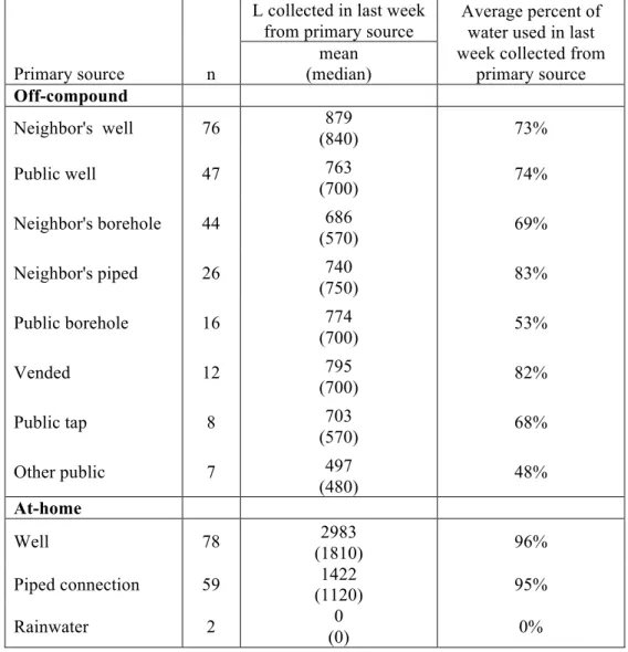
Table 10. Volume of water (L) collected in the last week from primary sources and as a percent of all water used, by primary source type ... 34
Table 11. Water collection trips made in the last week, and fraction of trips made on foot ... 35
Table 12. Percent of households using at least one other source in the last week ... 36
Table 13. Back-up sources for three most common primary sources ... 37
Table 14. Respondents without at-home sources that always selected or rejected certain types of sources in all choice tasks* ... 38
Table 15. Respondents with at-home sources that always selected or rejected certain types of sources in all choice tasks ... 38
Table 16. Description of primary and hypothetical source attribute variables for households without an at-home source ... 43
Table 17. Multinomial logit models for selected source ... 45
Table 19. Average marginal effects of increases in collection time for
households without an at-home source ... 47 Table 20. Mixed logit model for selected source including source attributes
of reliability and health risk interacted with asc ... 48 Table 21. Mixed logit models with household characteristics ... 51 Table 22. Responses to the question “When you are deciding which water
source to use, which factor would you say is most important?” ... 52 Table 23. Linear regression of total liters of water used in the last month
for households without at home primary water sources ... 57 Table 24. Sub-set analysis excluding choice tasks with inconsistent preferences ... 106 Table 25. Logit regression for preferring current source over a hypothetical
source for households without an at-home primary source ... 107 Table 26. Logit regression for preferring hypothetical source A over hypothetical source B .... 107 Table 27. Mixed logit models with a conservative estimate of walk time
for households without at-home sources. ... 108 Table 28. Correlation between independent variables - households
without an at-home source ... 109 Table 29. Correlation between independent variables - households
with an at-home source ... 109 Table 30. Conditional logit model for asc interactions with health risk and reliability ... 110 Table 31. Description of primary and hypothetical source variables
for choice experiment for households using an at-home source ... 111 Table 32. Mixed logit model (lognormal price distribution) of preferred
source for households using an at-home source ... 112 Table 33. Average marginal effects of increases in collection time for
households with an at-home source ... 112 Table 34. Mixed logit models with collection time assumed to be 5
LIST OF FIGURES
Figure 1. Number of studies at each phase of the screening process ... 5
Figure 2. Example choice card translated into English ... 22
Figure 3. Estimated total water gathering times in minutes from primary sources for households without an at-home source ... 30
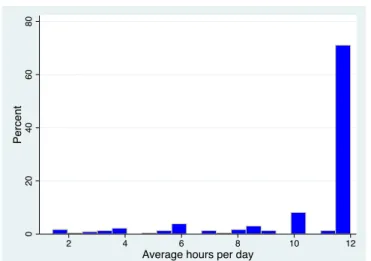
Figure 4. Average hours per day that water is available from primary sources for households without an at-home source ... 32
Figure 5. Cumulative change in probability of source selection as price per 20L jerrican increases ... 46
Figure 6. Cumulative change in probability of source selection as collection time increases ... 47
Figure 7. Monthly coping costs frequency distribution for sample households without at-home sources ... 53
Figure 8. Composition of water costs by income group for households without at-home sources ... 54
Figure 9. Composition of water costs by not at-home primary source type ... 55
Figure 10. Average coping costs for households walking to their primary source ... 55
Figure 11. Coping cost per L and quantity of water used by households without at-home primary sources ... 56
Figure 12. Households where the questionnaire was piloted neighboring the study region ... 63
Figure 13. Water sources: Thewa swamp, borehole, and a shallow well ... 63
LIST OF ABBREVIATIONS
asc alternative specific constant CL Conditional logit
CM Choice modeling
CV Contingent valuation
F Fahrenheit
HEV Heteroscedastistic extreme value
HH Household
IIA Independence of Irrelevant Alternatives JMP Joint Monitoring Program
Kg Kilogram
Ksh Kenyan Shillings
L Liters
MNL Multinomial logit
MXL Mixed logit
n sample size
NL Nested logit
UNICEF United Nations Children’s Fund USD United States Dollars
1. Introduction
Of the 768 million people globally without access to improved drinking water, 83% live in rural areas (WHO, 2013). To extend access to rural populations, it is important to understand their preferences. For example, are people willing to walk to public taps? Would they rather pay more for water and not have to walk as far? Or would they prefer to pay for at-home piped connections? Hope (2006) explains, “policy that fails to respond to the preferences of the target beneficiaries is likely to allocate resources, capacity, and funds inefficiently and ineffectively.” In Kenya, only 54% of rural people have access to improved sources of drinking water compared to 83% of urban dwellers (WHO, 2013). This makes Kenya a particularly important region to study the water source preferences of rural people. I use a stated preference choice experiment to investigate how water source and household attributes affect water source selection. The primary research questions guiding this work are:
(1) How do rural Kenyans trade-off time and price when selecting a water source? (2) How do rural Kenyans value time spent collecting water?
(3) How are household characteristics (such as income and education) relevant to water source choice?
2. Literature review
The first study of water source choice in developing countries, Drawers of Water: Domestic Water Use in East Africa, was published in 1972. Despite increased international funding for improved water supply in developing countries in the years since (Thompson et al., 2001), surprisingly few studies have focused on household water source choice. General
consensus in the literature is that both water source and household characteristics are relevant to household source choice (Nauges & Whittington, 2009). However, there is little agreement regarding the relative importance of varying source attributes and household characteristics in these decisions. Both stated and revealed preference methods have been used to study water source choice. Stated preference methods, such as contingent valuation and choice experiments, present respondents with a hypothetical question or set of choice tasks and have been used widely in developing countries (Whittington, 2010). In contrast, revealed preference methods, such as the travel cost method, estimate valuation of non-market goods based upon observed behavior.
2.1 Systematic review methods
The goal of this systematic literature review is to identify which water source attributes and household characteristics have been found to be important to household water source choice, as well as weaknesses in the methods used in existing literature. Published peer-reviewed
domestic water source choice and choice modeling based on a variety of water source attributes. Studies on water used for agriculture were excluded from the review. Literature focused on assessing water demand was not included (see Nauges & Whittington, 2009 for a detailed review of this literature).
Information sources for the review included four databases with varying temporal coverage: Web of Science (1955-present), EconLit (1969-present), Academic Search Complete (1975-present), and Scopus (1996-present). There were no geographic, year, or language restrictions on the search. One study selected for the review was not written in French and was translated to English for review using Google Translate. All searches were conducted on March 20, 2014.
2.2 Identified studies
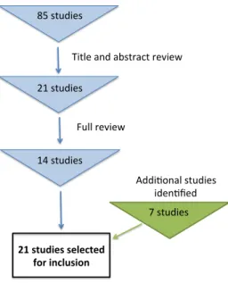
The primary search identified eighty-five studies focused on water source choice after duplicates were removed. Out of the four databases, the Web of Science database identified the most articles (n=42). Based on a review of the titles and abstracts, twenty-one articles on source choice met the inclusion criteria for methods (choice modeling) and topic (water source).
Figure 1. Number of studies at each phase of the screening process
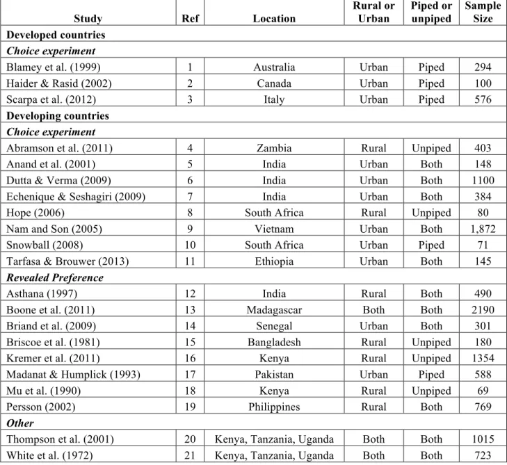
Table 1 provides characteristics of the twenty-one studies included in the review organized by developed or developing country and method (choice experiment, revealed preference, or other).
85#studies#
21#studies#
14#studies# Full#review#
Title#and#abstract#review#
Addi8onal#studies# iden8fied# 7#studies#
Table 1. Characteristics of studies included in the systematic review
Study Ref Location
Rural or Urban
Piped or unpiped
Sample Size Developed countries
Choice experiment
Blamey et al. (1999) 1 Australia Urban Piped 294 Haider & Rasid (2002) 2 Canada Urban Piped 100 Scarpa et al. (2012) 3 Italy Urban Piped 576 Developing countries
Choice experiment
Abramson et al. (2011) 4 Zambia Rural Unpiped 403
Anand et al. (2001) 5 India Urban Both 148
Dutta & Verma (2009) 6 India Urban Both 1100 Echenique & Seshagiri (2009) 7 India Urban Both 384 Hope (2006) 8 South Africa Rural Unpiped 80 Nam and Son (2005) 9 Vietnam Urban Both 1,872 Snowball (2008) 10 South Africa Urban Piped 71 Tarfasa & Brouwer (2013) 11 Ethiopia Urban Both 145 Revealed Preference
Asthana (1997) 12 India Rural Both 490
Boone et al. (2011) 13 Madagascar Both Both 2190 Briand et al. (2009) 14 Senegal Urban Both 301 Briscoe et al. (1981) 15 Bangladesh Rural Unpiped 180 Kremer et al. (2011) 16 Kenya Rural Unpiped 1354 Madanat & Humplick (1993) 17 Pakistan Urban Piped 588
Mu et al. (1990) 18 Kenya Rural Unpiped 69
Persson (2002) 19 Philippines Rural Both 769 Other
Thompson et al. (2001) 20 Kenya, Tanzania, Uganda Both Both 1015 White et al. (1972) 21 Kenya, Tanzania, Uganda Both Both 723
2.3 Developed country results
that the gender of the household member interviewed should not greatly affect willingness to pay estimates. Studies of source choice often rely on an interview with only one member of a
household to represent preferences of the household unit, so this finding is reassuring. The other two developed country studies, conducted in Australia and Canada, assessed preferences
regarding new municipal water supply sources. Blamey et al. (1999) found that Australian respondents supported water recycling for outdoor use but not for indoor uses. In Canada, Haider & Rasid (2002) found cost to not be a significant predictor of source choice; instead respondents were more concerned about improved taste and pressure.
2.4 Developing country results
Table 2 presents the modeling method used, a summary of the findings, and strengths and weaknesses of the research design for each selected study from a developing country. The
Table 2. Modeling method, findings (source attributes and household characteristics), and strengths and weakness of research design and modeling for selected studies.
Abbreviations used in the table: HH= household, IIA = irrelevance of independent alternatives. Models: MNL = multinomial logit, CL = conditional logit, HEV = heteroscedastistic extreme
value, NL = nested logit, CM = choice modeling, MXL = mixed logit Study Ref Model
Source attributes
HH characteristics
Design
strengths Design weaknesses
Stated choice experiments
Abramson et al. (2011)
4 CL
price (-) quality (+) time (-)
Sig: income
not Sig:
education, HH size, gender
Compared WTP with willingness to borrow and to work
Hypothetical options; Recommend a revealed preference study;
Did not check IIA
Anand et al. (2001) 5
CL, NL
price (-) convenience
Sig: current source; satisfaction with current source Nested logit relaxes IIA assumption
Found that nested models not appropriate; Other modeling challenges Dutta &
Verma (2009)
6 CL, NL price (-) quality (+)
Sig: HH size, consumption, education Nested logit relaxes IIA assumption Parametric assumptions; Confounding from unobserved factors Echenique & Seshagiri (2009)
7 CL
price (-) quality (+) availability (+) pressure (+)
Sig: income, HH size, literacy, toilet ownership
not Sig: education
Estimated WTP for specific attributes
Assump. that valuation is sum of attributes; Ordering of choice tasks influenced results
Hope
(2006) 8
MNL, latent class convenience (+) quantity over quality -- Latent class modeling relaxes IIA assumption; Fewer assumptions about data
Did not look at HH characteristics; Specific to the poor, rural study sites
Nam and Son (2005)
9 CL
price (-) quality (+) pressure (+)
Sig: income
not Sig: age, gender Compared CV and CM; Estimate WTP for specific attributes
Did not check assumption of IIA
Snowball
(2008) 10
CL, HEV price (-) quality (+) discolor (-) interruptions (-)
Sig: HH experienced service disruptions
Also used HEV which allows the distribution of error terms to vary across attributes
Small sample (n=71);
Only wealthier HHs
Tarfasa & Brouwer (2013)
11 MXL
price (-) quality (+) quantity (+) reliability (+)
Sig: income, gender
not Sig:
education, age, HH composition
Table 2, continued
Study Ref Model Source attr. HH characteristics Strengths of design Weaknesses design
Revealed preference studies
Asthana
(1997) 12 CL
price (-) distance (-)
Sig (for safe source):
% female, female edu;
Sig (for yard tap): income, HH size
not Sig: male education
Compared HHs with and without piped water
relatively large sample size
IIA assump. not checked; No preference
heterogeneity with CL
Boone et
al. (2011) 13 CL distance (-)
Sig: education, HH asset ownership
Large sample size Both rural and urban population
IIA assump. not checked; No preference
heterogeneity with CL; No data on quality or quantity
Briand et
al. (2009) 14 probit
price (-) quality (+)
Sig: wealth, widow is head of house, HH size, sources available to HH, literacy
Took advantage of policy aimed to extend service to poor
Only studied private connection vs public standpipe decision
Briscoe et al. (1981) 15
pairwise
compar-isons
quality (+)
for poor HH:
distance (-), conflict (-)
Sig: wealth
didn't look at other HH characteristics
Early study in applying consumer theory to water source choice
No discrete choice model used;
Assumed same preferences for wealth groups
Kremer et al. (2011) 16
CL, MXL
quality (+) distance (-)
Sig: latrine ownership, mothers education
not Sig: diarrhea rates, asset ownership
Spring protection randomly assigned; Compared revealed pref with CV
Possible recall error for self-reported travel times; Focus on one type of source (natural springs)
Madanat & Humplick (1993)
17 MNL
for drinking:
quality (+)
for bathing: pressure (+), reliability (+)
Sig: male education, ownership of storage facilities
not Sig: HH size
Choice analyzed by water use type; Also analyzed connection decisions
IIA assump. not checked; No preference
heterogeneity; Sequential estimation biased sig upwards
Mu et al.
(1990) 18 MNL
price (-) time ( -)
Sig:% female
not Sig: income, education
Developed discrete choice model for water; Compared to traditional water demand model
Attributes are all source-specific;
Small sample (n=69); IIA assump. not checked
Persson
(2002) 19 CL, NL
price (-) distance (-)
Sig: HH size
not Sig: income
Nested logit relaxes IIA assumption; Checked for consistency with utility maximization
Not enough data to estimate the 'full' nested model;
No pref heterogeneity
Other Thompson et al. (2001) 20 index from ranking quality (+) convenience (+)
Sig: wealth, education, HH size, urban
Longitudinal study compared to Whiteet al. from 30 years earlier
No discrete choice model used, instead semi-structured interviews
White et al. (1972) 21
index from ranking
price (-)
quality (+) Sig: wealth, HH size
First study of water source choice in developing countries; Three countries studied
Source attributes
All of the articles that looked at price found households to prefer water sources with lower prices. Quality of the water was also an important attribute to both piped and unpiped households (Refs 4, 7, 9-11, 14-16). Water quality was defined in most studies as likelihood of health risk due to microbial contamination. In rural Kenya, Kremer et al. (2011) found that households using multiple sources began collecting a greater fraction of their water from springs when those springs were protected to reduce contamination of the water. The relative importance of quality may depend on wealth or whether the household has a piped connection. In South Africa, Hope (2006) found that households without piped connections valued quantity of water over quality improvements whereas Snowball et al. (2008) found “bacteria count” to be the most important attribute for urban households with piped connections.1 In Bangladesh, Briscoe et al. (1981) also found quality concerns, in this case including taste, smell, and color, to be a factor in water source choice for wealthier households.
For households without piped water connections, distance to the source is of primary concern. Studies in Kenya, India, the Philippines, and Madagascar found distance or walking time to the source to be the main predictor of household source choice (Refs 12-14, 18, 19). The one study that investigated whether possible conflict with other users had an impact on source choice found it to be important in Bangladesh, particularly for the poor (Ref 15). In South Africa and India, studies have found that many households prioritize the convenience of having a piped connection in their compound (Refs 5, 8).
For households that have a piped connection, reliability is a major concern (Refs 7, 11). Pressure is also important for households with piped connections (Ref 9), but may vary in
importance by type of water use. In Pakistan, Madanat & Humplick (1993) found reliability and pressure to be the prioritized attributes in sources used for bathing.
Household characteristics
Household income or wealth was an important factor in source choice in eight of the studies (Refs 7, 9, 11, 12, 14, 15, 20, 21). However, three studies did not find income or asset ownership to be associated with household water source choice (Refs 16, 18, 19). The financing mechanism to obtain an improved source may influence whether income is a factor in water source choice. Abramson et al. (2011) found that wealthier households in Zambia preferred to pay for water source improvements in cash, while lower-income households preferred “loan and labor financing”. Studies in India, Pakistan, and Senegal found households with piped water systems to have higher incomes (Refs 12, 14, 17). There is a relatively extensive literature on willingness to pay for improved water sources, including piped connections. Abramson et al. (2011) conducted a meta-analysis of twenty-one contingent valuation studies estimating willingness to pay for improved water sources. The main findings of the meta-analysis are that willingness to pay for improved water sources is lower in rural compared to urban areas and cost recovery of rural water service improvements is usually infeasible.
statistically significantly associated with water source choice (Refs 12, 16). One study in Pakistan found male education to impact water source choice (Ref 17), but another in India found that male education was not a factor (Ref 12).
In households without a piped connection, studies in India and Kenya have found the fraction of women in the household to influence water source choice (Refs 12, 18). This relationship is generally attributed to the fact that women do the majority of water hauling, so additional female household members provide the household with greater carrying capacity. In Senegal, Briand et al. (2009) found that households led by widows were more likely to be connected to the piped system. The proposed explanation for this finding was that women were interested in the convenience of an at-home piped connection and widows made the household decision about whether to connect. Household size has also been found to be positively associated with the likelihood of obtaining a piped connection (Refs 12, 14), as has a greater proportion of men household members (Refs 12).
2.5 Discussion of the literature
responsible for the majority of water collection, the fraction of females within a household may influence source choice in providing greater carrying capacity.
In their review of water demand in developing countries, Nauges & Whittington (2009) write that, “the literature on household water source choice, especially in rural areas, is still in its infancy”. This systematic review confirms that there is much to be learned regarding how
3. Theoretical framework
Choice modeling is based on utility maximization, or the theory that consumers maximize their personal utility subject to their budget constraint. In the context of a choice experiment, respondents are expected to select the alternative within the choice set that
maximizes their utility. Varying levels of attributes are bundled into alternatives and respondents are assumed to derive utility based upon the attribute levels within each bundle (Lancaster, 1966). The choice set must: (1) have mutually exclusive alternatives; (2) be exhaustive; and (3) have a finite number of alternatives (Train, 2009). The choice set used in this research meets these criteria in that respondents were required to select one preferred water source from a choice set including two hypothetical sources and their current source (the status quo).
The household member responsible for the majority of water decisions was selected as the respondent for the household questionnaire and choice experiment. I thus assume that the respondent interviewed can represent the preferences of the household (as in Mu et al., 1990). Following McFadden (1974), if a household h has J water sources available to it, the household chooses source j if and only if the utility of source j is higher than that of source i:
Uhj≥ Uhi assuming i ≠ j & i, j ∈ J (1)
Since the household’s complete utility function is unobservable, the utility of household h is decomposed into an observed component and a random component:
And the probability that household h selects water source j can be written:
Phj = Prob(Vhj + εhj≥ Vhi + εhi ) for all i ≠ j & i, j ∈ J (3)
If the error term (εhj) is assumed to be identically, independently distributed extreme
value (or Gumbel), the conditional logit model for the probability that household h selects water source j is:
𝑃!! = !!!"
!!!!!" (4)
The conditional logit model is based upon the assumption that the property of independence from irrelevant alternatives (IIA) is met. IIA is often explained by the red-bus blue-bus problem. When a second bus of a different color is added to a transportation choice set, the probability that a decision maker selects one of the other alternatives should not change, assuming that the buses are identical other than in color. However, in this case, the conditional logit model will overestimate the probability that the decision maker will select one of the buses and under-estimate the probability of selecting a non-bus transportation option. This red-bus blue-bus problem illustrates a scenario in which IIA is not a valid assumption.
The Hausman specification test can be used to determine whether the conditional logit model meets the assumption of IIA. The null hypothesis in this test is that there is no systematic difference between the coefficients estimated in a model including all of the alternatives
𝑃!! = !"#!’!!!
!! !"# !’!!" f(β) dβ (5)
This represents a weighted average of the logit form based on the weights in f(β). The coefficients can vary, which permits preference heterogeneity.
Returning to the observable utility, Vhi, we consider it to be a function of water source
attributes, represented by the vector Xhi, as well as household characteristics, represented by the vector Zh. Assuming that the utility function is additive in terms of source and household characteristics, the observable utility Vhi can be written:
Vhi = γXhi + αjZh (6)
where γ represents the coefficients on the water source attributes (constant across all sources and
households) and αj represents source-specific coefficients on the household characteristics. In this work, the main water source attributes of interest (Xhi) are price and time. Other source attributes such as health risk, likelihood of conflict, and reliability also likely affect household water source choice. However, the choice experiment was meant to be simple for enumerators to administer and for respondents to answer, so price and time were the only water source attributes varied for the hypothetical choices. Additional attributes are modeled to the extent possible given that these attributes varied only across households’ current sources. The household attributes (Zh) modeled are monthly income, whether the respondent has at least a primary education, and the proportion of women in the household.
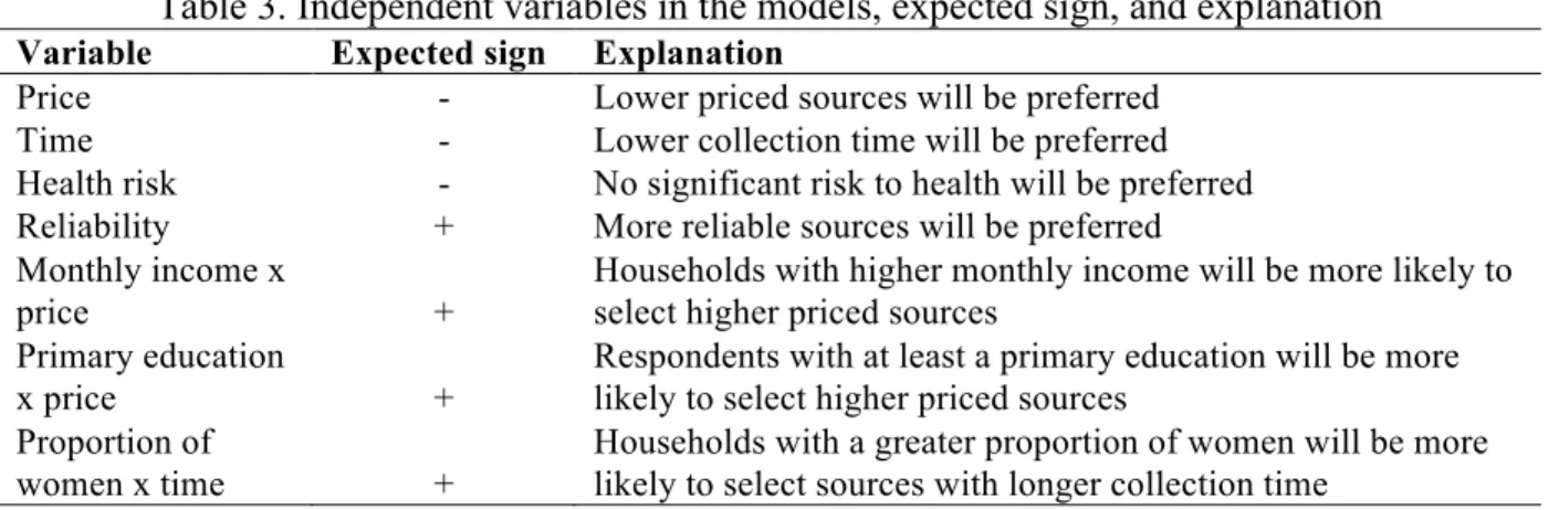
Table 3 provides the variables and expected signs on model coefficients. Based upon findings in the source choice literature, I expect cheaper sources and those with lower collection times to be preferred. I also expect a negative coefficient on health risk, as I predict that
expect to find that wealthier and more educated respondents are less price sensitive. Mu et al. (1990) found that households with a greater proportion of women were more likely to select sources associated with greater amount of collection time in Ukunda, Kenya. I thus expect the number of women in the house to be positively associated with the selection of water sources with longer collection time.
Table 3. Independent variables in the models, expected sign, and explanation
Variable Expected sign Explanation
Price - Lower priced sources will be preferred Time - Lower collection time will be preferred Health risk - No significant risk to health will be preferred Reliability + More reliable sources will be preferred Monthly income x
price +
Households with higher monthly income will be more likely to select higher priced sources
Primary education
x price +
Respondents with at least a primary education will be more likely to select higher priced sources
Proportion of
women x time +
Households with a greater proportion of women will be more likely to select sources with longer collection time
Given that utility is assumed to be additive based upon source attributes, I expect
households to reject sources that have a clearly “worse” bundle of attributes compared to another alternative in the choice set. I refer to “preference inconsistency” as instances in which a
household selects a source that appears worse based upon observable attributes. This may be due to attributes of a households’ current source that we have not observed (such as smell or
4. Research design
4.1 Fieldwork
Fieldwork was conducted in the areas (most commonly referred to as “sub-locations”) of Kianjai, Mutionjuri, Machaku, and Nairiri in Meru County, Kenya. Approximately 140 miles north east of Nairobi, the Kenyan capital, Meru County borders Mount Kenya national park. The elevation is approximately 5,000 feet and average annual temperatures range from 62-69°F. Considered one of the most fertile parts of Kenya, this agricultural area produces staple crops, such as wheat, potatoes, and maize, as well as cash crops including tea, coffee, and bananas. Rice is sold for 85 Ksh (~1 USD) 2 per kilogram and the price of maize is 30 Ksh (~ 0.35 USD) per kilogram (or 2.2 pounds). Average annual rainfall is fifty-four inches and there are a variety of surface and ground water sources. Local government and non-governmental organizations, such as the Red Cross, are currently expanding access to piped systems and public taps, making this area a particularly interesting site to study rural water source choice.
These four sub-locations were selected based on site visits that found a diverse array of water source options. The household questionnaire was informed by discussions with local residents and piloted in areas neighboring the study sites. See Appendix B for photographs of the study region taken during site selection and piloting. Piloting of the survey instrument aimed to identify potential problems with the survey or flag confusing sections to be clarified. The final questionnaire included sections on water sources used by respondents, other water sources available in the area, sanitation options, demographics, income sources, and the choice
related decisions so that the respondents would be knowledgeable about the water sources available and used by the household.
During August 2013, a team of six enumerators and two field managers completed 388 household surveys. The household interviews were conducted in Meru, the local language. Pairs of enumerators were matched with a village elder within each sub-location for help finding respondent households. Sampling was cross-sectional based on transect walks of each area. If no one was available in a selected house, callbacks were scheduled. Enumerators made three
attempts to interview selected households, after which the household was replaced with the next closest household. Table 4 provides the number of households interviewed per sub-location and the total households in the sub-location. Unfortunately, information on how many households were replaced was not collected, nor was the number of households that refused to participate in the study.
Table 4. Interviews conducted and total number of households in each sub-location Sub-location Interviews conducted Total Households
Kianjai 141 1091
Mutionjuri 129 992
Machaku 44 341
Nairiri 74 581
4.2 Choice experiment design
The following hypothetical scenario was read to each respondent to introduce the choice experiment:
Now I would like you to imagine that a group is planning to install several new water points in your area to improve your access to water. The group could be the government or it could be a non-governmental organization. These water points could be boreholes or public standpipes from the piped network. If they install only a few water points, people might have to walk further and wait longer to collect water. If they install more, people might walk shorter distances and have to wait less. Installing these water points is expensive, however. Suppose <the group> will need to charge people who use the water points to recover their costs and properly maintain the water points. If they install more points, they may need to charge more per jerrican.
You just told me that the primary source for most purposes right now was <primary source from previous question>. In addition to that source, I want you to imagine you have two new water points available for you to use. You should assume that quality of the water from the new water point is excellent and safe for drinking. You should also assume that the reliability of the new water point would be excellent: it would always have good pressure and you could collect from it whenever it is convenient for you. Finally, you should assume that using the source would not cause any conflict with other water users.
The two new water points differ only in the cost you would have to pay per jerrican, and the total amount of time it would take you to walk to the source, wait, fill your container and return. Here is the first task I would like you to think about.
The enumerator then showed the respondent the choice task card, explained the attributes associated with each hypothetical new water point, and asked if the respondent had any questions. An example choice task card is shown in Figure 2.
*TASK 99*
New water point A New water point B Your current source
Total time to walk to source, wait, fill container
and return home 10 minutes 5 minutes
Cost per 20L jerrican
1 Ksh per 20L jerrican 0.25 Ksh per 20L jerrican
If these three sources were available to you right now, which source would you most prefer to use? Remember that the two new sources have excellent quality, reliability, and using them would not cause conflict. Which source would you least prefer to use?
The enumerator marked on the questionnaire which of the three sources the respondent most preferred and which source was least preferred. The baseline situation was the status quo. A hypothetical baseline was avoided given the difficulties associated with administering these surveys well and comprehension challenges for respondents (Whittington, 2010). The term “preferred source to use” was intended to mean the source that the respondent would use
exclusively as their primary water source and this is how the question was posed to respondents in the Meru language.3
Each household completed four choice tasks: a “block” of three tasks presented in random order and one task answered by all households. The experiment was based on a full factorial design of two three-level attributes: price of 0.25, 1, or 3 Ksh and total water collection time of 5, 10, or 30 minutes. These attribute levels were chosen to be close but slightly lower than average current source prices and collection times so that they would be tempting to
respondents. Because the choice experiment was not the focus of the survey effort, unfortunately these attribute levels were not pre-tested.4 From the full factorial, obvious choices in which one source dominated the other source with regards to both price and time were eliminated. For example, if Source A had a price of 1 Ksh and a time of 5 minutes and Source B was priced at 3 Ksh and took 30 minutes, Source A was considered to dominate Source B. We then eliminated symmetric duplicates to yield the final nine choice tasks, which were divided equally into the three “blocks”. In addition to a randomly selected block, all respondents were presented with a
3 The Meru translation of “If these three sources were available to you right now, which source would you most prefer to use?” is: “Guntu kuu kuthatu gwa gutaa ruuji gukeethirwa gukionekana kirigwe onendi, ni kuriku ugichaalaa kuruki ya kungi?”
4 As a result, the hypothetical times chosen (5, 10, 30 minutes) were less than half of average current
task including one source with the lowest time and lowest price and another source with the middle time and middle price (as shown in Figure 2 above.) With one of the two hypothetical sources dominating the other in both time and price, this task served as a simple comprehension check for the choice experiment. The task was also intended to determine whether the most attractive hypothetical source might tempt households with at-home sources, due to the high reliability and excellent water quality of the hypothetical sources. The four choice tasks were presented to respondents in random order. Table 5 provides the ten choice tasks and associated attribute levels.
Table 5. Full choice experiment design
task ID
Source A Source B
Price (Ksh)
Time (min)
Price (Ksh)
Time (min) 11 0.25 10 1 5 12 0.25 30 1 10
13 3 5 1 30
21 0.25 10 3 5 22 0.25 30 3 5 23 3 10 0.25 30 31 0.25 30 1 5
32 3 5 1 10
5. Results
5.1 Respondent and household characteristics
Table 6. Socioeconomic and demographic characteristics of sample households by sub-location (mean with standard deviation below in parentheses or percentage of the sample)
Household or respondent characteristic Kianjai n=141 Mutionjuri n=129 Machaku n=44 Nairiri n=74
Household size (2.3) 5.3 (2.2) 5.6 (1.6) 4.8 (2.2) 6 .0
Years of respondent education 7.6 (3.9) 7.9 (3.8) 6.75 (3.5) 7.1 (43.9)
Monthly Income (Ksh) 44,598 (36,174) 63,572 (114,847) 35,143 (28,830) 54,451 (73,319) Weekly per capita food expenditures 554
(414) 378 (223) 323 (238) 376 (235) Acres of land owned 2.0
(2.3) 2.1 (2.8) 1.8 (1.0) 2.0 (2.3) % of respondents with job for wages 26% 22% 5% 5% % of households owning livestock 88% 90% 95% 96%
Ninety-seven percent of respondents have a sanitation facility on their compound and, of these, 13% share this facility with others outside of their household. Nearly all households use a pit latrine. Only two respondents reported to have a water-sealed flush toilet, which were
reported to cost between 11,000-30,000 Ksh (128-349 USD). About half of respondents’ pit latrines have a slab and about a quarter are ventilated. Three quarters of respondents are somewhat or very satisfied with their pit latrine and the most frequent complaint is the smell.
5.2 Water sources
purchased from vendors, and surface water sources are considered “unimproved” sources. Fieldwork was conducted in the dry season so rainwater was generally not available. Ninety five percent of households reported that they use the same primary source during the dry season for drinking, washing in the home, bathing, cooking, watering outside the home, and other
productive uses. Women are primarily in charge of water collection; in over three quarters of households, a woman collected the most water in the last week.
Sixty one percent of households have a primary source outside of their compound (or “not at-home”) including neighbors’ sources and public wells, boreholes, and taps.
Approximately one third of households have a primary source located on their compound or “at-home”, which includes shallow wells, piped connections, and rainwater. Households without an at-home source have a lower average monthly income (44,411 Ksh or 516 USD) compared to households that have at-home sources (63,174 Ksh or 735 USD).
The remaining 3% of respondents report that water purchased from vendors is their primary source of water. While vended water is not a common primary source, 80% of
households reported that it is possible to purchase water from a vendor who delivers to the home. Two thirds of households had purchased water from a vendor at some time in the past and one fifth reported to have purchased water from a vendor in the last week.
Table 7. Number of households using each type of primary source (n), primary source dry season collection time, and price per 20 liter jerrican (including households that do not
pay for their water) Collection time (min)
mean (median)
Price/ 20L jerrican (Ksh) mean
(median) Primary source n
Off-compound
Neighbor's well 76 86 (66)
1.4 (2)
Public well 47 194
(70)
3.6 (5) Neighbor's borehole 44 66
(50)
2.4 (2) Neighbor's piped 26 55
(47)
1.8 (2) Public borehole 16 103
(70)
2.3 (2)
Vended 12 0*
(0)
9.9 (10)
Public tap 8 149
(145)
3.3 (2.5) Other public sources 7 151
(120)
2.6 (1)
At-home
Well 78 2*
(2)
0* (0) Piped connection 59 2*
(2)
1.2 (0.98)
Rainwater 2 0*
(0)
0* (0) * Values that are assumed rather than based on household questionnaire responses
Figure 3. Estimated total water gathering times in minutes from primary sources for households without an at-home source (excluding an outlier of 800 minutes)
The average price for a 20 L jerrican from a neighbor’s well is 1.4 Ksh (0.02 USD). Public sources have higher average prices: per 20 L jerrican, the average price for public wells and public taps are both over 3 Ksh. Water purchased from vendors who deliver to the household costs 9.9 Ksh per 20 liter jerrican on average.
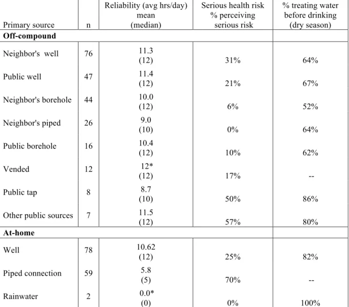
Table 8 presents reliability, quality perceptions, and frequency of water treatment for each type of primary source. Reliability is calculated as the average hours per day the source is available across a week, censored at a maximum of 12 hours/day.5 Vendors are assumed to be available 12 hours/day and rainwater is assumed to be available 0 hours/day given that data was collected during the dry season. At-home wells are assumed to be available all the time, unless the respondent reported that the well did not have water in August, the month that the survey was conducted. Twelve percent of households using at-home wells reported that the well water was not available and reliability was thus coded as 0 hours/day. Respondents were asked about perceived serious health risk for all the sources. Table 8 also presents the percent of respondents using a given primary source that believe that drinking from the source poses a serious risk to
5 Censoring at 12 hours per day was done to avoid confusion about availability of sources at night time.
For example, some households may have interpreted the question such that they reported neighbor’s
0
5
10
15
20
Pe
rce
n
t
0 100 200 300 400
their health. The final column in table 8 presents the percent of households using each primary source who report to treat the water before drinking. Unfortunately, households were not asked about treatment of water from at-home piped connections or purchased from vendors.
Table 8. Primary source dry season reliability (censored at 12 hrs/day), perceived serious health risk from drinking, and water treatment
Primary source n
Reliability (avg hrs/day) mean
(median)
Serious health risk % perceiving
serious risk
% treating water before drinking
(dry season)
Off-compound
Neighbor's well 76 11.3
(12) 31% 64%
Public well 47 11.4
(12) 21% 67%
Neighbor's borehole 44 10.0
(12) 6% 52%
Neighbor's piped 26 9.0
(10) 0% 64%
Public borehole 16 10.4
(12) 10% 62%
Vended 12 12*
(12) 17% --
Public tap 8 8.7
(10) 50% 86%
Other public sources 7 11.5
(12) 57% 80%
At-home
Well 78 10.62
(12) 25% 82%
Piped connection 59 5.8
(5) 70% --
Rainwater 2 0.0*
(0) 0% 100%
* Values that are assumed rather than based on household questionnaire responses
reliability of primary water sources for households without an at-home primary water source. About two thirds of these respondents have a primary source that is available close to at least 12 hours/day on average.
Figure 4. Average hours per day that water is available from primary sources for households without an at-home source (averaged across a week and censored at 12 hours/day)
Perceptions of serious health risk vary considerably across the sources but the majority of respondents report to treating their water before drinking. About a third of respondents using a neighbors’ well as their primary source perceive a serious health risk from drinking this water. About half of respondents using public taps or other public water points as their primary source believe that water from these sources poses a serious risk to health. Neither of the households reporting rainwater as their primary source perceive the water to be a health risk but both treat the water with chlorine. Few households perceive the public and neighbors’ boreholes to pose a serious health risk. It is interesting that none of the households using a neighbor’s piped system perceived a serious health risk from drinking the water while 70% of households using their own piped connection perceive a health risk from the water.
0
20
40
60
80
Pe
rce
n
t
2 4 6 8 10 12
Table 9 gives the frequency of different methods of water treatment by monthly income groups: low (median 15,500 Ksh or 180 USD), middle (median 35,000 Ksh or 407 USD), and high (median 69,640 Ksh or 810 USD). Unfortunately the questionnaire did not include
questions about treatment of at-home piped connections or water purchased from vendors, so this table excludes the seventy-one respondents who used this type of primary source. Treatment rates are relatively similar across these three income groups, though middle- and high-income households are more than three times as likely to both boil their water and add chlorine compared to the low-income group.
Table 9. Fraction of respondents by income group using water treatment methods Treatment type
(n=303)
Monthly Income Classification low middle high
no treatment 33% 31% 31%
chlorine 11% 11% 12%
boil 50% 43% 46%
stand and settle 2% 3% 0%
boil and add chlorine 3% 10% 11%
Table 10 presents the volume of water collected in the last week from each primary source, as well as the average fraction of water used from that primary source, relative to water used from all sources in the last week. For households using at-home wells and piped
Table 10. Volume of water (L) collected in the last week from primary sources and as a percent of all water used, by primary source type
L collected in last week
from primary source Average percent of water used in last week collected from
primary source Primary source n (median) mean
Off-compound
Neighbor's well 76 879
(840) 73%
Public well 47 763
(700) 74%
Neighbor's borehole 44 686
(570) 69%
Neighbor's piped 26 740
(750) 83%
Public borehole 16 774
(700) 53%
Vended 12 795
(700) 82%
Public tap 8 703
(570) 68%
Other public 7 497
(480) 48%
At-home
Well 78 2983
(1810) 96%
Piped connection 59 (1120) 1422 95%
Rainwater 2 (0) 0 0%
Table 11. Water collection trips made in the last week, and fraction of these trips made on foot Total trips to collect water
(HHs making >0 trips/wk) Average percent of trips that are walking Primary source n
mean (median)
Off-compound
Neighbor's well 71 40
(35) 68%
Public well 42 30
(21) 55%
Neighbor's borehole 42 28
(26) 53%
Neighbor's piped 26 37
(35) 82%
Public borehole 27 35
(35) 55%
Vended 6 9
(6.5) 98%
Public tap 7 22
(25) 55%
Other public 5 29
(28) 40%
At-home
Well 8 31
(36) 69%
Piped connection 10 20.5
(8.5) 62%
Rainwater 1 6
(6) 0
Table 12. Percent of households using at least one other source in the last week Primary source n
% using at least one other source in the last week Not at-home
Neighbor's well 76 39% Neighbor's borehole 44 45% Neighbor's piped 26 27% Public water point 91 51%
Vended 12 58%
At-home
Private piped 59 24%
Private well 78 14%
Rainwater 2 100%
Households were also asked what back-up source they would use if their primary source was unavailable. Table 13 provides the frequency of back-up source types reported by
households with the three most common primary sources (neighbor’s well, well at-home, piped connection at-home).6 A public borehole or neighbor’s borehole are the most common back-up sources for households using a neighbor’s well as their primary source. For households with wells at home, a neighbor’s well is the back-up source for a majority of households. The most common back-up source for households with a piped connection at home is a public well (32%) followed by a neighbor’s well (23%) or public borehole (15%).
Table 13. Back-up sources for three most common primary sources Primary source
Secondary source
Neighbor’s well (n=73)
Well at home (n=73)
Piped at home (n=53)
Bottled water 0% 1% 0%
Neighbor's borehole 16% 10% 4%
Neighbor's piped 11% 4% 8%
Neighbor's well 11% 59% 23%
Other public 14% 4% 2%
Public Borehole 18% 7% 15%
Private well 0% 0% 6%
Public tap 0% 0% 8%
Public well 1% 3% 32%
Rainwater 7% 3% 2%
Surface water 1% 0% 2%
Vended 21% 10% 9%
5.3 Choice experiment and validity checks
these statistics for households that use at-home piped connections, wells, or rainwater as their primary source.
Table 14. Respondents without at-home sources that always selected or rejected certain types of sources in all choice tasks*
Kianjai n=76
Mutionjuri n=106
Machaku n=11
Nairiri n=56
All n=249 Always chose current source (status quo) 20% 5% 0% 0% 8% Always chose cheapest source 28% 12% 20% 16% 18% Always chose lowest time source 3% 2% 0% 0% 2% Always rejected current source (status quo) 48% 32% 20% 76% 46% Always rejected most expensive source 15% 8% 0% 44% 18% Always rejected highest time source 43% 32% 20% 75 44% *note: data on least preferred source were missing for some households without at-home sources. For the “always rejected” sample sizes are: Kianjai n=75, Mutionjuri n=104, Machaku n=10, and Nairiri n=55.
Table 15. Respondents with at-home sources that always selected or rejected certain types of sources in all choice tasks
Kianjai
n=65 Mutionjuri n=22 Machaku n=33 Nairiri n=18 n=138 All Always chose current source (status quo) 75% 50% 30% 28% 54% Always chose cheapest source 72% 55% 21% 6% 49% Always chose lowest time source 74% 50% 33% 33% 55% Always rejected current source (status quo) 8% 14% 0% 22% 9% Always rejected most expensive source 11% 5% 3% 6% 7% Always rejected highest time source 43% 32% 21% 0% 30%
connections, or rainwater) as their primary source results in the analysis of 973 choice tasks completed by 244 different respondents.
Inconsistent preferences
Three types of inconsistent preferences were possible. First, respondents could select the dominated hypothetical source in the choice task completed by all respondents. Twelve
respondents selected this dominated source, which suggests that these respondents may have not understood the choice experiment.
Second, respondents could select their current source even though one of the hypothetical sources appears to have a “better” bundle of attributes. In 722 of the 973 total choice tasks at least one of the hypothetical sources dominated the respondent’s current source based upon the attributes studied. In 7% of these tasks (forty-nine tasks representing twenty-six different households) the respondent selected their current source even though the hypothetical option appeared to be “better”. In three-quarters of these “preference inconsistencies”, the respondent’s current source was a neighbors’ source. In 417 choice tasks both of the hypothetical sources appeared to dominate the current source. In 5% of these instances (nineteen choice tasks, representing eleven different households) respondents selected their current source. Although these preference choices appear inconsistent within the choice experiment, the respondent’s choice could be due to status quo bias or some other characteristic of his or her current source that we did not observe.
Robustness checks
To test the reliability and accuracy of the choice experiment data, I conducted four types of robustness checks: (1) sub-set analysis of only the choice tasks in which there were no preference inconsistencies; (2) analysis of a choice between each hypothetical source and the household’s current source based on the ranking data; (3) comparison of the two hypothetical source options based on the ranking data; and (4) sensitivity of the results to assumptions about collection time. Detailed results from the four robustness checks summarized below are provided in Appendix D.
First, I conducted a sub-set analysis excluding “preference inconsistencies”, as defined in the previous section. This excluded sixty-one choice tasks: twelve tasks in which the respondent selected the dominated hypothetical source in the choice task completed by all respondents and forty-nine tasks in which at least one of the hypothetical sources appeared to dominate the current source, yet the respondent preferred their current source. The coefficients and statistical significance are very similar to the model that includes these sixty-one “inconsistent preference” tasks. The magnitude of the coefficient on price is slightly smaller and magnitude of the
coefficient on time slightly larger compared to the mixed logit model including choice tasks that revealed inconsistent preferences.
Second, I analyzed the data as a choice between each hypothetical source and the household’s current source based on the ranking data. Each choice task completed by a
respondent led to two observations in this data set, Hypothetical Source A versus current source and Hypothetical Source B versus current source, resulting in a total of eight choices per
and reliability of the respondent’s current source were also included as independent variables. In this model, the coefficients on price and collection time are negative and statistically significant, as expected. When reliability and health risk are added to the model, neither of the coefficients on these variables is statistically significant and the coefficient on price is less statistically significant. While these logit models do not account for the full structure of the data, it is reassuring that the sign and significance of the price and time variables remain relatively consistent.
Third, I used the ranking data collected to compare relative rankings of the two hypothetical sources. Similar to the logit model used in the previous robustness check, I
calculated independent variables of price difference and collection time difference between the two hypothetical sources. Other source attributes (reliability and health risk) were constant across both hypothetical sources and could not be included in the model. This logit model yields coefficients on both price and time that are negative and highly statistically significant, as expected (p < 0.01).
significance of the coefficients does not change. The coefficient on price is smaller but the coefficient on time is virtually unchanged.
5.4 Variables and coding
Including highly correlated independent variables can be problematic in multinomial regression models,7 so I examined the correlation coefficients between source attribute variables. Appendix E provides the correlation matrices of these independent variables. The alternative specific constant (asc), equal to one for a respondent’s current source, and the variables of reliability and likelihood of conflict are all highly correlated because all of the hypothetical sources (asc=0) were very reliable and associated no chance of conflict. I also find also high correlation between collection time and asc because the hypothetical times presented in the choice experiment were substantially lower than most households’ current round-trip collection time. I would expect to see high correlation with health risk, which was assumed to be zero for the hypothetical sources. This correlation is somewhat lower, which can be explained by the low frequency of occurrence relative to the other variables. Because of the particularly high
correlation between likelihood of conflict and the other independent variables, it is excluded from the multinomial models.
Table 16 describes the coding of the variables used in subsequent multinomial logit regression models. The hypothetical sources were coded according to the time and price
presented on the task card. As given in the hypothetical scenario, the attribute of health risk was
7 If there is multicollinearity between variables, one of the variables must be dropped to run the model or
coded as 0 and reliability as 12 hours/day. Characteristics of the household’s primary source were coded according to the respondent’s responses in the questionnaire.
Table 16. Description of primary and hypothetical source attribute variables for households without an at-home source
Variable Description Hypothetical source
coding
Primary Source Coding
Time
Round trip walk time and waiting
5, 10, or 30 minutes (2*1 way walk time with full container)
+ (wait time)
Price Price of 20L jerrican Ksh 0.25, 1, or 3 otherwise, Ksh/20 L jerrican price 0 if doesn't pay
Health Risk
Perceived risk from drinking
0 0 = reported no or some health risk 1=reported serious health risk
Reliability
Average hours/day in a week (censored
at 12 hrs/day)
12 hours/day Average hours/day across the week
Vended: assumed 12 hours/day asc alternative specific constant 0 1
5.5 Multinomial regression models
As found in the systematic literature review, conditional logit models are used in the analysis of most water source choice studies. However, if the assumption of IIA is rejected based upon Hausman’s specification test, mixed logit models are preferred. Estimated using maximum simulated likelihood, mixed logit models generate a distribution of coefficients for the sample based upon respondent choices (Hole, 2007). The shape of these distributions must be specified, leading to the need for additional assumptions.
Source attributes
jerrican, and collection time. The conditional logit model is based on the assumption that all respondents have the same preferences and thus each coefficient is constant across the sample. For the two mixed logit models (Models 2-3), the mean and standard deviations of predicted coefficients are provided. Each maximum likelihood simulation used 500 Halton draws.8
The conditional logit model (Model 1) yields negative and statistically significant coefficients on collection time and asc. It is unexpected that the coefficient on price is not statistically significant. The negative coefficient on asc indicates that respondents prefer the hypothetical sources to their current source, which may reflect the importance of source
attributes other than price or time, such as quality or reliability. However, based on the Hausman test, the assumption of IIA does not hold: I reject the null that the difference in coefficients is not systematic when the current source alternative is dropped from the model (p<0.0001). This indicates that conditional logit models are not appropriate for these data, so I move onto mixed logit models.
The mixed logit models, assuming a normal distribution for all variables (Model 2) or a lognormal distribution for price (Model 3), yield negative, statistically significant coefficients on both price and time, as hypothesized. Under the assumption of a normal distribution for all variables (Model 2), the model estimates positive price and/or time coefficients for some of the respondents, but it is implausible that households would prefer higher prices or collection times. Lognormal distributions eliminate the chance of positive coefficients. The mixed logit model with a lognormal distribution for price (Model 3) has coefficients close in magnitude to those of Model 2, but the standard deviation of the price coefficients is an order of magnitude larger.
Unfortunately, the maximum likelihood function for models assuming a lognormal distribution for time would not converge. 9
Table 17. Multinomial logit models for selected source
distributions: normal price lognormal10
(1) (2) (3)
VARIABLES Conditional logit Mixed logit Mixed logit Price - mean -0.0964*** -0.882*** -1.003***
(0.0321) (0.125) (0.338)
Price - SD -1.089*** 1.843***
(0.161) (0.120) Time - mean -0.0230*** -0.182*** -0.225***
(0.00277) (0.0218) (0.0310)
Time - SD 0.113*** 0.163***
(0.0151) (0.0233) asc - mean -0.458*** -2.590* -2.775*
(0.150) (1.381) (1.605)
asc - SD 10.03*** 11.679***
(1.380) (2.070) Observations 2,886 2,870 2,870 Standard errors in parentheses
*** p<0.01, ** p<0.05, * p<0.1
All of these models rely on assumptions that can be questioned. The conditional logit results (Model 1) rely on the assumption of IIA. The mixed logit with all normal distributions (Model 2) permits respondents to have preferences for higher prices and collection times. The mixed logit model with a lognormal distribution for price still assumes a normal distribution for collection time, although it is unlikely that a person would prefer a greater collection time. Lognormal distributions also assume that there is a long tail, or in this case, large price coefficients for some respondents. Nevertheless, the mixed logit model with a lognormal
9 The model would not converge for a lognormal distribution for time, despite setting starting values
distribution for price is based upon the most plausible assumptions, so I proceed with the analysis using this model.
Table 18 and figure 5 show the average marginal effects of increases in price for
households without at-home sources.11 An increase in price from 1 to 3 Ksh per 20 liter jerrican decreases the probability of selection by 11% on average.
Table 18. Average marginal effects of increases in price of 20 L jerrican for households without an at-home source
Price (Ksh) Change in probability
0-1 -0.09
1-3 -0.11
3-5 -0.04
5-10 -0.04
Figure 5. Cumulative change in probability of source selection as price per 20L jerrican increases (with time and asc variables held constant)
Table 19 and figure 6 show the average marginal effects of increases in collection time for households without at-home sources. An increase in collection time from 20 to 40 minutes decreases the probability of selection by 15% on average.
11 To calculate marginal effects, I took the difference in probabilities that a source would be chosen at two
different attribute levels. Because the choice experiment data set is at the alternative-level, a random alternative within each choice task was selected to obtain the average probability for a given attribute
0% 20% 40% 60% 80% 100%
0 1 2 3 4 5 6 7 8 9 10
R
el
ati
ve
p
rob
ab
il
ity of
se
le
cti
on