USE OF R2 STATISTICS FOR ASSESSING GOODNESS-OF-FIT AND MODEL SELECTION IN THE LINEAR MIXED MODEL FOR LONGITUDINAL DATA
Jean Guilmond Orelien
A dissertation submitted to the faculty of the University of North Carolina at Chapel Hill in partial fulfillment of the requirements for the degree of Doctor in Public Health in the Department of Biostatistics (School of Public Health)
Chapel Hill 2007
©2007
ABSTRACT
JEAN G. ORELIEN: Use Of Pseudo-R2 For Assessing Goodness-Of-Fit and Model Selection in The Linear Mixed Model for Longitudinal Data
(Under the direction of Dr. Lloyd Edwards)
In the Linear Mixed Model (LMM), several R2 statistics have been proposed for assessing goodness-of-fit. However, the performance of these statistics has not been demonstrated. In this dissertation research, first we show that many of the 2
ACKNOWLEDGEMENTS
In the course of completing this dissertation, I am forever indebted to many family members, friends, colleagues and faculty in the school of Public Health at UNC. I am very thankful for my wife whose support has made it possible to put the time toward work and the pursuit of a doctorate degree knowing that she had everything under control on the “home front”. To my kids (Katina, Vladimir, Vijay and Valexa), I thank you for accepting that your dad has not spent as much time as he wanted with you while completing this degree and growing a small business. To my mom who wanted her son to be a doctor, this one is for you. I’m also
thankful for the support of my brother-in-law. To my brother Jonas, I am blessed to have you as a brother. Brother, this degree is proof that you too can reach high to achieve your dreams. Don’t ever give up on your dreams. To the rest of my family members, I thank you so much for the confidence you have in me. I thank all my friends who have understood that because of my busy schedule, I did not stay in touch as much as I should.
Last but not least, it was a privilege to learn from world class faculty at UNC. I’d like to thank members of my dissertation committee and in particular the chair Dr. Lloyd Edwards. Dr. Edwards, your class on Linear Mixed Model was the inspiration for this dissertation. A special thank you to Dr. Shoenback who has taught me everything I know about
TABLE OF CONTENTS
1 Literature Review ...1
1.1 Introduction ...1
1.2 The general linear mixed model ...3
1.3 The Concordance Correlation Coefficient ...4
1.3.1 Generalization of the CCC...5
1.3.2 Objections to the use of the CCC...7
1.3.3 The CCC as a goodness-of-fit statistic ...8
1.4 Pseudo-R2 Measures in Generalized Linear and Nonlinear Models ...9
1.4.1 Pseudo-R2 statistics for linear mixed models ...10
1.4.2 Marginal versus conditional ...15
1.4.3 Other approaches for GOF for generalized nonlinear models ...16
1.5 Adequacy of the Covariance Structure ...16
1.5.1 Graphical methods...16
1.5.2 Analytical methods ...18
1.6 GOF in the GLMM ...20
1.6.1 Relationship between the GLMM and the linear mixed model ...20
1.6.2 GOF statistics in the GLMM ...21
1.7 Conclusion...24
2 Fixed Effect Variable Selection in Linear Mixed Models Using 2 R Statistics...29
2.2 The Linear Mixed Model ...34
2.3 Proposed R2 Statistics in the LMM...36
2.3.1 Conditional versus marginal R2 Statistics ...41
2.4 Data Generation Techniques for Simulation Study ...42
2.5 Results of the Simulation ...43
2.6 Data Example ...45
2.7 Discussion ...46
2.8 Conclusion...48
3 2 R Statistics as Measures of external and internal consistency in the Linear Mixed Model ...55
3.1 Introduction ...56
3.2 The Linear Mixed Model ...59
3.3 Approaches for Developing R2 Statistics ...60
3.3.1 2 R based on comparing the Mahalanobis distance of the model to a null model ...60
3.3.2 R2 based on measures of agreement between observed and predicted values ...63
3.3.3 2 R based on comparing the variation explained by the model at hand to that of a null model ...64
3.3.4 R2 based on computing the variation explained by the model as a proportion of the variation in the outcome assuming that the fitted model is adequate ...66
3.4 New R2 Statistics ...68
3.4.1 New R2 statistics based on comparing the variation explained by the model at hand to that of a null model ...68
3.4.2 New R2 statistics based on computing the variation explained by the model as a proportion of the variation in the outcome assuming that the fitted model is adequate ...70
3.6 Example...75
3.7 Discussion ...76
3.8 Conclusion...78
4 Performance of Pseudo- 2 R Statistics in Detecting Misspecification in the Random Effects in Linear Mixed Models...93
4.1 Introduction ...94
4.2 The Linear Mixed Model ...97
4.3 Pseudo-R2 Statistics ...98
4.4 Data Generation Techniques...100
4.5 Data Analysis and Results ...101
4.6 Example: Schizophrenia Data ...103
4.7 Discussion ...105
4.8 Conclusion...106
LIST OF TABLES
Table 2.1 Summary of statistics reviewed ... 51
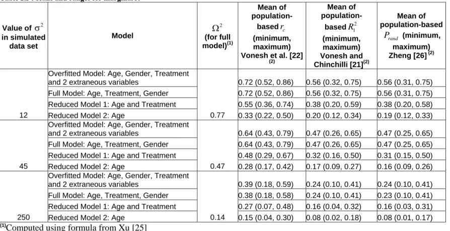
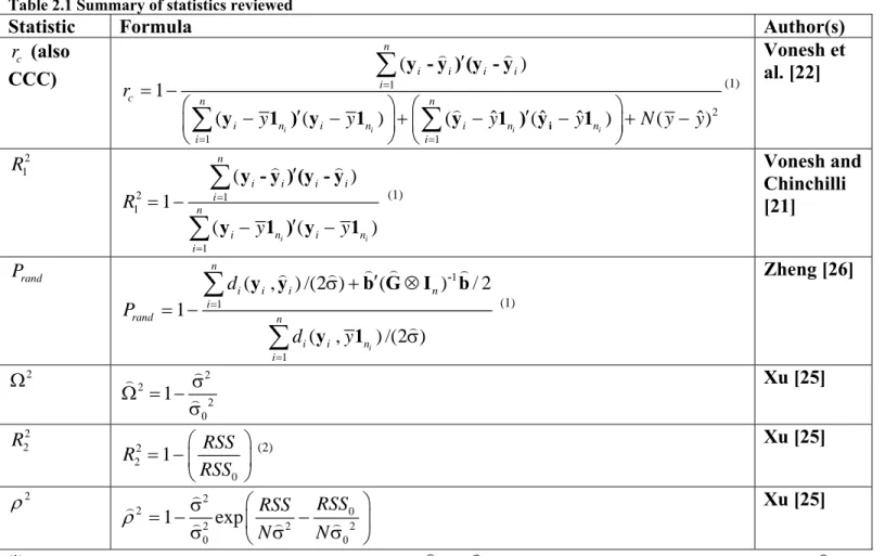
Table 2.2 Means and ranges for conditional R2 and R2 proposed by Xu [25] ... 52
Table 2.3 Means and ranges for marginalR2 ... 53
Table 2.4 Conditional R2 statistics and R2 proposed by Xu [25] on the dental data from Pothoff and Roy [15] ... 54
Table 2.5 Marginal 2 R for dental data of Potthoff and Roy [15]... 54
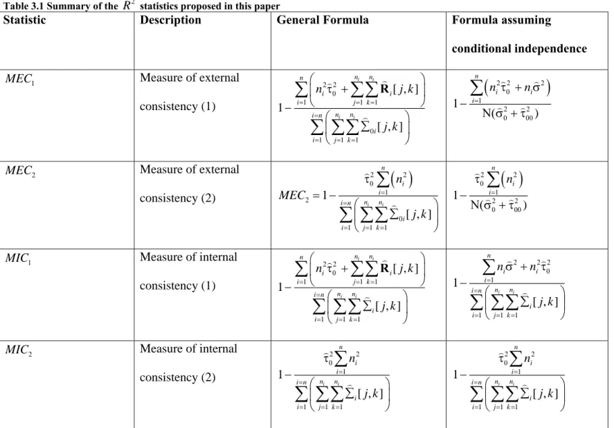
Table 3.1 Summary of the R2 statistics proposed in this paper ... 84
Table 3.2 Description of the data sets used in the simulation... 85
Table 3.3 Average and Interquartile range for the proposed R2 using only replicates where Hessian matrix and covariance matrix of random effects are positive definite (data sets with diagonal covariance matrix for the random effects) ... 86
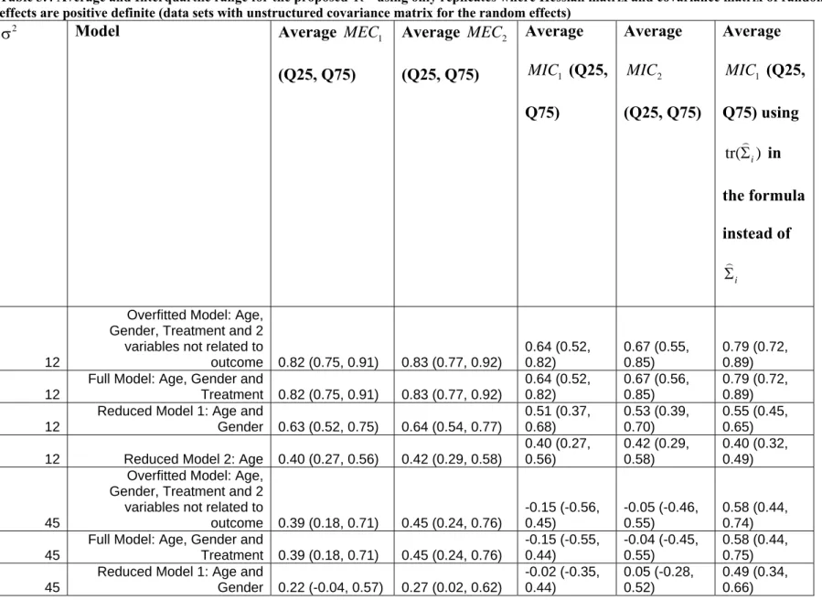
Table 3.4 Average and Interquartile range for the proposed R2 using only replicates where Hessian matrix and covariance matrix of random effects are positive definite (data sets with unstructured covariance matrix for the random effects) ... 87
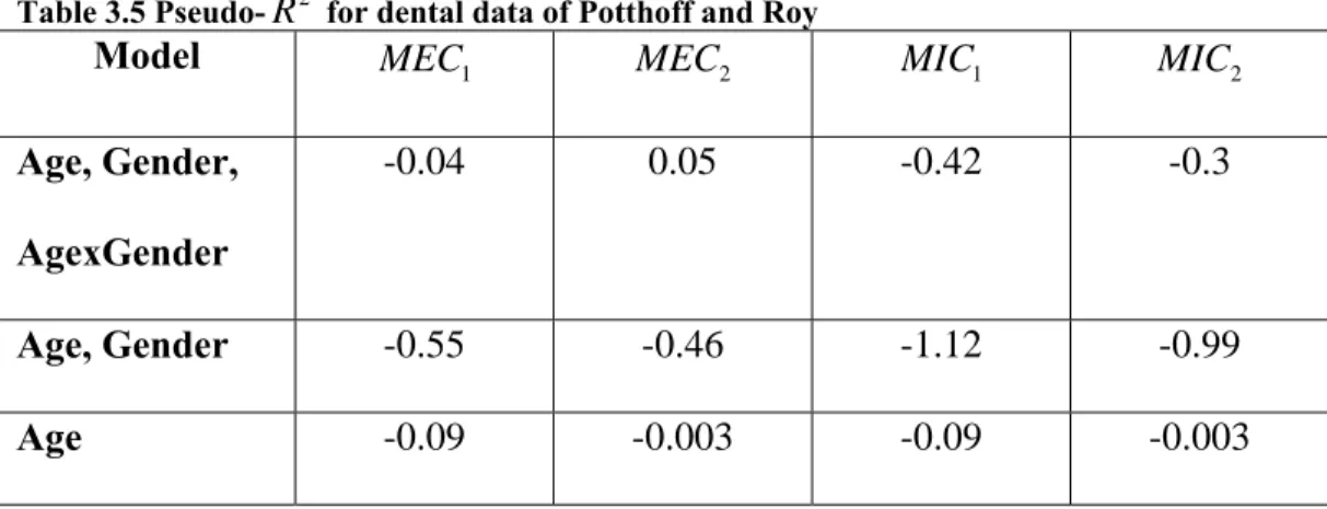
Table 3.5 Pseudo-R2 for dental data of Potthoff and Roy ... 89
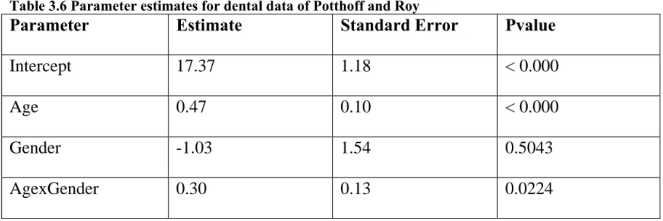
Table 3.6 Parameter estimates for dental data of Potthoff and Roy ... 90
Table 3.7 Covariance Parameter Estimates for dental distance data (full model) ... 91
Table 3.8 Distribution of dental distance by age and gender... 91
Table 4.1 Description of the data sets used in the simulation... 109
Table 4.2 Performance of the statistics MEC1 and MIC1 in assessing adequacy of random effects... 110
LIST OF FIGURES
1
Literature Review
1.1
Introduction
Few tools are available for assessing goodness-of-fit (GOF) in the linear mixed model. Traditional statistics such as the likelihood ratio test (LRT), the Akaike Information Criterion (AIC) introduced by Akaike (1974), or the Bayesian Information Criterion (BIC) by Shwarz (1978) require that two models be fitted to the data. For the LRT, the two models must be nested. The AIC and BIC can be used when the two models are not nested, though a non-nested mean structure violates the assumptions used to originally derive the AIC. However, in comparing the values of AIC or BIC, it is not clear what magnitude of difference constitutes a meaningful or significant one.
Recently, other statistics have been proposed in the statistical literature for assessing goodness-of-fit in linear mixed models. It is not clear which, if any, of these statistics
1.2
The general linear mixed model
Assume the following linear mixed model (Harville 1977, Laird and Ware 1982): i i i i i
y = Xβ+ Z b + e (1)
where i∈ {1, 2, ..., n}is the index for the independent sampling units (ISU) and
i
y is an ni×1 vector of observations from the ith independent sampling unit (subject),
i
X denotes an ni×p fixed effects design matrix for the ith subject, β is a p×1 vector of unknown, constant, fixed effect parameters,
i
Ζ denotes an ni×q random effects design matrix for the ith subject,
i
b is a q×1 vector of unobservable random effects for the ith subject, and
i
e denotes an ni×1 vector of unobservable within-subject error terms.
It is also assumed that bi has a multivariate normal distribution Nq( ,0 G) independent of ei, which has a multivariate distribution ( , )
i
n i
N 0 R .
i
i
E⎡ ⎤ ⎡ ⎤⎢ ⎥ ⎢ ⎥= ⎣ ⎦ ⎣ ⎦
b 0
e 0 and
i
i i
V⎡ ⎤ ⎡⎢ ⎥ ⎢= ⎤⎥
⎣ ⎦ ⎣ ⎦
b G 0
e 0 R ,
where G is a q q× unknown covariance matrix for the random effects and Ri is an
i i
n ×n unknown covariance matrix for the within-subject error terms. With these assumptions, we have Σi =V( )yi =ΖiGΖi′+Ri. In many applications, Ri is taken to be 2
i n
σ I , known as
the conditional independence assumption for the error term (Laird and Ware 1982). By stacking the vectors of responses and associated matrices, the mixed model can also be expressed as
where
1 2
( ′ | ′ | . . .| ′ ′n) =
y y y y is N×1 and
1
n i i
N n
=
=
∑
; X=(X X1′| ′2| . . .|X′ ′n) is N×p;1 2
( , ,. . ., n)
Diag
=
Ζ Ζ Ζ Ζ is N nq× ; andb = (b′1 |b′2 | . . .|b′ ′n) is nq×1 and
1 2
( ′ | ′ | . . .| ′ ′n) =
e e e e is N×1. The distributional assumptions are that b∼Nnq( ,0 G I⊗ n) independent of e∼NN( , )0 R , R=Diag(R R1, 2,. . ., Rn) is N×N. Also,
1 2
( ) ( , ,..., n)
V Diag
= =
Σ y Σ Σ Σ .
A brief overview of approaches to parameter estimation for the model in (1) is given by Ware (1985). The use of maximum likelihood (ML) and restricted maximum likelihood (REML) approaches for linear mixed models was first discussed by Harville (1977). Laird and Ware (1982) proposed a Bayesian approach to estimation and the use of the EM algorithm for both the Bayesian approach and the ML approach. Detailed formulae for computing ML and REML estimates using the EM algorithm with suggestions on how to speed convergence are given in Laird, Lange, and Stram (1987).
1.3
The Concordance Correlation Coefficient
Consider n pairs of independent measurements ( , )x yi i and for i≠ j, the pairs ( , x yi i) and ( , )x yj j are independent with ( )E xi = μx, ( )E yi = μy, V x( )i =σx2, V y( )i =σ2y, and cov( ,x yi i)= σxy. The CCC is denoted by ρcwhere:
(
)
22 2 2 2 2 2
2 1 ( ) ( ) i j xy c
x y x y x y x y
E x y σ
ρ
σ σ σ σ
⎡ − ⎤
⎢ ⎥
⎣ ⎦
= − =
+ + μ − μ + + μ − μ and its estimate is given in the equation
below by
12
2 2 2
1 2 2 ˆ ( ) c S
S S x y
ρ =
+ + − (2)
where 1 n i i x x = =
∑
, 1 n i i y y ==
∑
, 121 1 ( )( ) n i i i
S x x y y
n =
=
∑
− − , 12 21 1 ( ) n i i
S x x
n =
=
∑
− , and2 2 2 1 1 ( ) n i i
S y y
n =
=
∑
−Lin (1992) showed how to estimate sample sizes for computing the CCC. A discussion of other methods for assessing agreement is found in Lin, Hedayat, Sinha, and Yang (2002). Muller and Buttner (1994) provide a discussion of the different intraclass correlation coefficient (ICC) statistics used to assess agreement between measurements and how to make an appropriate choice.
1.3.1 Generalization of the CCC
curve model. One potential problem with this approach is the fact that there may be a limited number of variables available to use as covariates in modeling one measurement as a
function of the other. This approach would be impractical in the context of using the CCC as a goodness-of-fit statistic for linear mixed models. It is not clear how one would choose the covariates to model the predicted and observed values.
Vonesh, Chinchilli, and Pu (1996) proposed that an unweighted CCC denoted rc be used to assess goodness-of-fit for the generalized nonlinear mixed effect models. For these models, they formulate the CCC as follows:
1
2
1 1
( )
1
ˆ ˆ ˆ ˆ
( ( ) ( ( ) ( )
n
i i i i i
c n n
i i i i i i i
i i
r
y y y y N y y
=
= =
′ = −
⎛ − ′ − ⎞ ⎛+ − ′ − ⎞+ −
⎜ ⎟ ⎜ ⎟
⎝ ⎠ ⎝ ⎠
∑
∑
∑
iy - y ) (y - y
y 1 ) y 1 y 1 ) y 1
(3)
where n is the number of independent sampling units (or subjects), yi is the vector of observed values for the ith subject, yi =Xiβ+ Z bi iis the vector of predicted values for the ith
subject, y is the grand average of the predicted values, y is the grand average of the observed values, and N is the total number of observations.
The rc measures the percent agreement between observed and predicted values. A value of 1 corresponds to perfect agreement, and values close to 0 correspond to a lack of fit. Note that in their paper, Vonesh et al. (1996) erroneously gave the range for rc as being between -1 and 1.
raters for data that involve multiple measurements), their test is liberal, resulting in higher rates of rejection of the null hypothesis than the stated nominal type I error rate. The liberality of the test could be an artifact of using a distribution free approach to derive estimates. When only an intercept is included in the model, the estimates from Barnhart and Williamson (2001) and Lin (1989) are the same.
Remarking that the CCC is based on the squared function of distance, King and Chinchilli (2001) proposed a generalized CCC for both continuous and categorical data. The authors based their formula for the CCC on convex functions of distance. For categorical data, their class of estimators has similarities with the kappa and weighted kappa statistics. The choice of a particular distance function is akin to choosing a set of weights to estimate a weighted kappa. Their extended version of the CCC can be used in situations where there is an interest in estimating agreement for more than two raters or assays. Barnhart, Haber, and Song (2002) proposed an overall CCC for assessing interobserver variability when there are more than two observers. It turns out that the overall CCC that they proposed is equivalent to the generalized CCC of King and Chinchilli (2001) when the squared distance function is used.
1.3.2 Objections to the use of the CCC
Atkinson and Nevill (1997) object to the use of the CCC and other correlation
for assessing reproducibility, the CCC is nearly identical to a subset of coefficients in that group. Liao and Lewis (2000) urge caution when using correlation coefficients and advocate the need for an improved correlation coefficient.
1.3.3 The CCC as a goodness-of-fit statistic
The recommendation for use of the CCC is based on the observation that predicted and observed values are similar to a set of measurements from two instrumentations: a gold standard (observed values) and another set of measurements (predicted values). However, for models such as generalized linear mixed models in which observations from the same subject are correlated, Vonesh et al. (1996) did not take into consideration the fact that the
assumptions underlying the CCC, as outlined by Lin (1989), are not applicable. Three assumptions of the CCC are that (a) the two sets of measurements come from a bivariate normal distribution, (b) the two sets of measurements have equal variances, and (c) each pair of measurements for an individual observation are independent of all other pairs. While Lin (1989) showed that the CCC is robust to deviation from normality, the fact that observations from a generalized linear mixed model are correlated raises questions about the use of the CCC for such models. Given the issues of the underlying assumptions of the CCC being violated for correlated models, simulations would be desirable to ensure that the CCC is a suitable goodness-of-fit statistic in such models. Other issues not addressed by Vonesh et al. (1996) include transformations and models in the class of generalized non-linear mixed models, such as logistic regression, for which the observed values are not continuous.
Zheng (2000) recommended the use ofrc,
2 1
example is given by Zheng (2000) where he analyzed data on growth measurement published by Pothoff and Roy (1964), with age, gender, and their interaction as potential predictors. The analysis of the data showed that high values of the rc were obtained from any model that included age as an explanatory variable. Even when other statistically significant terms are removed from the model, the value of the rc remained relatively unchanged at 0.99. The fact that his computations yielded high values of the rceven when important terms were removed was not a cause of concern. This was a demonstration to him that the rc and the other three statistical measures that he proposed could discriminate between “statistical significance” and “practical importance” (Zheng, 2000). The possibility that there could be a problem with the rc and the other statistics he proposed was not explored. This should have been a
consideration in light of the remarks by Atkinson and Nevill (1997) that the rc, like other intraclass correlation measures, is sensitive to sample heterogeneity. It should be noted that if indeed there is an issue with the inability of rc to discriminate when other significant
variables are missing from the model, then the other statistics proposed by Zheng (2000) are likely to suffer the same deficiency. Although values for these statistics were not as high as the rc, when significant terms were removed, they too exhibited little change.
1.4
Pseudo-
R
2Measures in Generalized Linear and Nonlinear Models
Various R2 statistics have been proposed in generalized linear models. Some of these statistics are specific to a subclass of models and would not be applicable to the generalized linear mixed model. For example, various statistics have been proposed for logistic
distributions. In section 3.1, we focus on statistics that have been proposed specifically for generalized linear mixed models. Statistics that have been proposed for other generalized linear models and that can be applied to linear mixed models are discussed in section 3.2.
1.4.1 Pseudo-R2 statistics for linear mixed models
Besides the rc, Vonesh and Chinchilli (1997) proposed a statistic that we denote
2 1
R for assessing GOF in a generalized linear mixed model.
2 1 1 1 ( ) 1 ( ( ) i i n
i i i i i
n
i i i i
i R y y = = ′ = − ′ − −
∑
∑
y - y ) (y - y
y 1 ) y 1
(4)
This statistic is the counterpart to the traditional R2 in linear models and as such lends itself to ease of interpretation. However, R12 does not explicitly take into account the random components of the model and no simulation results were offered.
Zheng (2000) proposed two other pseudo-R2 measures besides the CCC for linear mixed models. The first one, denotedDrand is the same statistic as R12. However, it is referred to by Zheng (2000) as the proportional reduction in deviance. Although Drand is similar to
2 1
R , expression for it is given in (5) as it will be useful to simplify the expression for the other statistic proposed by Zheng (2000).
, 1 , 1 ( ) 1 ( ) n
i i i i
rand n
i i i i d D d y = = = −
∑
∑
y y y 1where i∈ {1, 2, ..., n}is the index for the ISU and y is the grand average of the observed values. Let ( , ; )L μ σ y denote the joint log-likelihood given the predictors and random effects, where μ=Xβ+ Zb. The numerator in equation 5,
, 1
( , ) 2( ( ; ) ( ; ))
n
i i i i i i i
i
d L L
=
= − ,σ − σ
∑
y y y y y y is defined as the deviance under the model athand and the denominator ,
1
( , ) 2( ( ; ) ( ; ))
n
i i i i i i i
i
d y L y L
=
= − ,σ − σ
∑
y 1 1 y y y is defined as thedeviance under the null model.
Another statistic proposed by Zheng (2000) is Prand, the proportional reduction in penalized quasi-likelihood (PQL).
1
1
( , ) /(2 ) ( ) / 2
1
( , )
n
i i i n
i
rand n
i i i i d P d y = = ′
σ + ⊗
= −
∑
∑
-1
y y b G I b
y 1
(6)
where
1
( , ) /(2 ) ( ) / 2
n
i i i n
i
d =
′
σ + ⊗
∑
y y b G I -1bis defined as the negative of the PQL,
b is the estimated vector of random effect parameters for all subjects, and G is the estimated covariance for the random effect parameters.
values for lack of fit and perfect fit. However, with these statistics the suitability of a “penalty term” over others needs to be demonstrated.
Xu (2003) proposed two statistics, in addition to the traditional R2 (R12) of Vonesh and Chinchilli (1997), for explaining the variations in a linear model: a statistic denoted r2 that measures the proportion of explained variation and a statistic denoted ρ2 that measures the proportion of explained randomness. The statistic r2 is derived from the fact that for the model in (1), the variability in the dependent variable yithat is not explained by the covariates (both fixed and random) is V( V( )
i
i i i σ n
2
⏐ ) = =
y X, b e I and the total variance of
i
y under a “null” model that assumes that the covariates have no effect is ( )
i
i n
V y = σ02I . The statistic r2 is given by
2
1
r
2 2 0
σ = −
σ and estimates
2 V( )
1
V( ) ij
ij
y
y
Ω = − | X, b ,
where j ∈ {1, 2, . . ., }ni so that yij is the jth element of yi, σ2
is the estimate of σ2
for the model at hand, and σ02 is the estimator for the residual variance of a “null” model. The null model could take the following form:
0 0
i iβ ibi i
y = 1 + 1 + u (7)
where β0 is an unknown fixed coefficient, b0i is an unknown random coefficient that has a normal distribution with mean 0, and ui is the unobservable within-subject random error term for the model (that is, equation 7 represents a model with fixed and random effect intercepts).
00 0
i iβ i
y = 1 + u (8)
where β00 is an unknown fixed coefficient and u0i is the unobservable within-subject random error term for the model (a model with a fixed effect intercept and no random intercept).
Explained randomness was first introduced by Kent (1983). Xu (2003) defines the randomness of a random variable Y as a monotonic transformation of its entropy,
exp[ 2 ( )]− I θ , where ( )I θ =E[log ( ;p y θ)] is the expected log-likelihood. Under the linear mixed model in (1), residual randomness is defined as
( ij| ) exp{ 2 [log ( ij )]}
D y X,b = − E p y | X,b . The proportion of explained randomness is then given as:
2 ( )
1
( )
ij
ij
D y
D y
ρ = − *
0 | X,b
| b ,
where D y( ij| b*0) is the expected log-likelihood of a null model [such as in (7) and (8)]. For the model in (1) and the null model in (7), it can be shown that an estimator of ρ2 is:
2 0
2 2
1 exp RSS RSS
N N
ρ 22
0 0
⎛ ⎞
σ
= − ⎜ − ⎟
σ ⎝ σ σ ⎠ (9)
where RSS is the residual sum of squares for the model in (1) and RSS0 is the residual sum of squares under model (7). The statistic ρ2 takes values between 0 and 1. In the absence of random effect terms from the model, it can be shown that ρ2 is equal to theR2of traditional linear models.
in terms of values of 2 1 V( ) V( )
ij
ij
y
y
Ω = − | X, b . He conducted a simulation with 100 replicates
for two cases: (a) 50 clusters with 5 observations per cluster and (b) 10 clusters with 25 observations per cluster. Data were simulated for different values of the “strength” of the fixed and random effects terms. For each set of simulated data, values of Ω2 could be computed exactly. The results of the simulations show that r2, ρ2, and R12 tend to give reasonable estimates of Ω2. For large clusters, the three statistics yield almost similar results. With smaller clusters, ρ2 andR1
2
tend to overestimate Ω2.
It should be noted that there are several limitations to the simulation results proposed by Xu (2003). Besides the small number of replications (100), the simulations did not address the ability of the statistics to discriminate overfitting or the effect of excluding significant covariates from the model. That is, it would be useful to ascertain how the statistics vary when there is overfitting (overestimation of Ω2 would be expected) or how they vary when important covariates are excluded (underestimation of Ω2 would be expected provided that the model does not include additional explanatory variables that exhibit a spurious
relationship with the outcome). Another issue with the simulations is that they did not
include sufficient variation of the fixed effect and random effect terms. Specifically, it would be desirable to determine how well these statistics estimate Ω2
when (a) the fixed effects account for a small proportion of the variability in the outcome relative to the random effects and (b) the fixed effects account for a large proportion of the variability in the outcome relative to the random effects.
The difference between explained residual variation and explained risk was described by Korn and Simon (1991). According to these authors, “explained risk” is “a way of
quantifying how much better predictions are when using the covariates compared to when not using them.” On the other hand, “explained residual variation” defined as the
proportional decrease in residual variation incorporates the “explained risk” and GOF (“applicability of the model to the data”).
1.4.2 Marginal versus conditional
Vonesh et al (1996) and Vonesh and Chinchilli (1997) discussed the concept of conditional versus marginal R2. For rc and R12, when the computations of the predicted values in the formula of these statistics involve the random effects (yi =Xiβ+ Z bi i), they are referred to by Vonesh et al (1996) and Vonesh and Chinchilli (1997) as conditional R2. On the other hand, when the computation of the predicted values in the formula of these statistics involve only the fixed effect components (yi =Xiβ), these statistics are referred to as
marginal R2. While the concept of conditional versus marginal R2 was introduced for rc
1.4.3 Other approaches for GOF for generalized nonlinear models Various approaches have been proposed in the statistical literature on pseudo-R2 for generalized linear models or a subclass of generalized linear models, such as logistic,
Poisson, and survival models. A good review of pseudo-R2 measures for logistic regression is given in DeMaris (2002). Similar measures for Poisson models are given in Cameron and Windmeijer (1996), Mittlbock and Waldhor (2000), and Heinzl and Mittlbock (2003). For survival models, pseudo-R2 measures were proposed by Graf and Schumacher (1995), Schemper and Stare (1996), Xu and O’Quigley (1999), Schemper (2000), Henderson, Jones, and Stare (2001), and O’Quigley and Xu (2001). For GEE models, no equivalent pseudo-R2
was uncovered in our literature search. However, GOF tests have been proposed by Barnhart and Williamson (1998), Horton et al. (1999), and Pan (2001) for binary outcomes and Pan (2002) for any GEE model.
Many of the approaches described in the previous section for linear mixed models were first proposed either for generalized linear models as a whole or for a subclass of generalized linear models. In particular, the equivalent of Drand for generalized linear models was first proposed by Cameron and Windmeijer (1996) and then by Zheng and Agresti (2000). Similarly, the measure of explained randomness was first proposed for survival models by Kent and O’Quigley (1988) and Xu and O’Quigley (1999).
1.5
Adequacy of the Covariance Structure
1.5.1 Graphical methods
those that can be used as diagnostic tools. We will restrict our attention in this review to diagnostic tools for determining the adequacy of the covariance matrix once a model has been fitted. For a review of graphical exploratory analysis techniques helpful in selecting a parsimonious covariance structure for fitting the model in (1), the reader is referred to
Diggle, Liang, and Zeger (1994), Dawson, Gennings, and Carter (1997), Zimmerman (2000), and Pourahmadi (2002). In addition to exploratory analysis consisting of plotting the
observations of each subject versus time, Weiss and Lazaro (1992) proposed plotting the residuals in a similar manner. This is an “omnibus” type of goodness-of-fit similar to the plotting of residuals versus predicted values to ascertain the adequacy of the model and to detect outliers. However, Weiss and Lazaro (1992) recognized that their graphical approach does not address the issue of the adequacy of the covariance structure and that additional graphics are needed.
Grady and Helms (1995) proposed graphical plots that can be used as model selection tools but also as a way to assess the adequacy of the covariance structure. The basic approach derived from their paper would consist of fitting a cell means model to the data with an unstructured covariance structure. The estimated covariance structure would then be plotted to ascertain which covariance structure best fits the data. The plot they suggested consists of plotting actual values of (covariance or correlations) as a function of lag time between
looking visually at the graphical plots. The closeness of the covariance of the fitted model to that of the cell means model would be an indication of a good fit.
1.5.2 Analytical methods
Two analytical approaches were proposed by Vonesh et al. (1996) to assess the adequacy of the covariance structure in generalized nonlinear mixed effect models. One of these tools is an R2 type statistic similar to rc denoted the variance-covariance concordance correlation, ( ).r ω This statistic measures the distance, scaled to 1, between the estimated covariance matrix of β from the model at hand and the “sandwich” covariance matrix estimator proposed by Liang and Zeger (1986). Vonesh et al. (1996) argued that since the covariance of β based on the “sandwich” estimator and the one based on the assumed structure of Σi (the covariance matrix of yi) will converge to the same limit if the assumption is correct, it makes sense to compare the goodness of fit of Σi to V( )yi by comparing how close the two estimators of the covariance of β are to each other. The other tool proposed by Vonesh et al. (1996) is a pseudo-likelihood ratio test (PLRT) to determine if the estimated covariance matrix is significantly different from the robust covariance
estimator.
The statistic for ( )r ω is given by:
2 2
2
|| ( ) || || ||
( ) 1
|| || || ||
r
p
2 2
ω = − =
|| + || +
ω- h (ω- h)
ω h ω , (10)
{
}
vech= -1/2 -1/2 R
ω Γ Γ Γ . Γ is the covariance estimate of β under the assumed covariance
structure and ΓR is the robust estimator of the covariance of β, ( )h=vech Ip , where
p=dim(β).
Vonesh and Chinchilli (1997) noticed that while ( )r ω could be useful for detecting gross differences between the assumed covariance structure of yi and its true value, “it is less useful to detect moderate but important suggestions.” The authors suggest that the pseudo-likelihood ratio test they have developed be used instead. That test statistic is given by:
(
)
{
ln| ln| trace}
n p
λ = | − | + -1 −
R R
Γ Γ Γ Γ (11)
Under the null hypothesis of Ho: var( )yi =Σi, the test has an approximate chi-square distribution with (p p+1) / 2 degrees of freedom. It should be noted that the degrees of freedom are based on an asymptotic likelihood ratio test and is the difference between the number of parameters that would have to be estimated assuming an unstructured covariance structure and the number of parameters assuming a more parsimonious model. So, the degrees of freedom for the test would be expected to be less than (p p+1) / 2. Results from a limited simulation (only 400 replicates) of this test were provided. The simulation results showed that the pseudo-likelihood ratio test performs well when yi has a multivariate normal distribution. The test may not be valid if yi follows a moderately (such as a multivariate T distribution) to heavily skewed distribution. Besides the small number of replications for the simulation, the results were based on a 2 × 2 covariance structure, which may affect
1.6
GOF in the GLMM
In developing other GOF tools for linear mixed models, one approach is to review similar GOF in other classes of models. Such a review will help determine if new GOF in the linear mixed models can be patterned after the GOF from other classes of models. GLMM is one of the likeliest candidates because every GLMM can be expressed as a linear mixed model and because of the existence of many GOF statistics for GLMMs.
1.6.1 Relationship between the GLMM and the linear mixed model Assume a GLMM:
Y = XΞ+ E (12)
where:
Y (N x p ) is an array of N random row matrices, {Yi}, each 1 x p and mutually independent,
ε
Y X= Ξ,is the N x matrix for the dependent variables which is assumed to be known and fixedq
X ,
is the x matrix of regression coefficients that are unknown, unknowable and fixedq q
Ξ ,
( )
V Y′ = ⊗I Σ (block-diagonal covariance matrix), and ( i)
V Y′ =Σ.
Note that the model in (12) can be written as a linear mixed model:
( )
( )
( )
x
1 1
1 1
x ) x 1
1 1 x ( )
... ...
vec ... ... ... ...
... p
i xq xq
xq i xq
i pq p
xq xq i p pq
1 ( 1
⎡ ⎤
⎢ ⎥
⎢ ⎥
′ = ⎡⎣ ⎤⎦ +
⎢ ⎥
⎢ ⎥
⎢ ⎥
⎣ ⎦
i
X O O
O X O
Y Ξ E
O O X
where Xi corresponds to the i
th
It should be pointed out that the resulting linear mixed model has the following characteristics:
• Every “subject” has the same number of observations; that is, there are no missing data within subjects.
• Observations within “subjects” are correlated but the “subjects” are mutually independent.
Hence, because of the limitations above, while every GLMM can be written as a linear mixed model, the inverse is not necessarily true.
1.6.2 GOF statistics in the GLMM
A review of GOF statistics for the GLMM is provided by Cramer and Nicewander (1979). The authors discussed seven statistics that can be used for assessing GOF. Only four of the seven statistics are commonly used (refer for example to Huberty 1994 or Tatsuoka and Lohnes 1988). These four statistics are Roy’s largest root (RLR), Pillai-Bartley trace (PBT), Hotelling-Lawley trace (HLT), and Wilks (W). To give expressions for these statistics, we first need to define the Wilks lambda criterion (Wilks, 1932) commonly denoted as Λ.
Let Ep p× be the error sum of squares and cross products (SSCP) matrix, that is,
p N N p
p p× ′× ×
E = (Y - Y) (Y - Y) , and let H be the hypothesis matrix (in the context of GOF, this is equivalent to testing that there is no effect or no relationship between the outcomes and the predictor variables, so that Hp p× corresponds to the between sum of squares matrix). Thus, we have Hp p× =[Yp N′× YN p× − py yp×1 1×′ p], where the i
th
average of the elements of Yi, the ithrow of Y. Let T = H + E (that is, T is the total sum of squares and cross products matrix about the mean).
The Wilks lambda criterion is defined as Λ =|Η|
|Τ|
PB is defined as the trace of HT−1, RLR is the largest eigenvalue of HT−1, and HLT is the trace of HE−1. The statistic W takes different forms depending on the author. Cramer and Nicewander (1979) define W as 1− Λ1/s, Huberty (1994) defines W as 1− Λ, and Tatsuoka and Lohnes (1988) use W = Λ. In the remainder of this document, we will use W = − Λ1 1/s.
Cramer and Nicewander (1979) show that these four statistics are functions of the canonical correlation. Given two set of variables Y and X, a measure of multivariate association between the two sets of variables can be obtained by considering the linear combination of the Y variables that has the greatest multiple correlation with the X variables. It can be shown that the coefficients for the X variables that maximize the matrix of correlations between the two sets of variables are the right eigenvectors of a matrix Mx (Mx is a function of the matrices of correlations among the X and Y variables and the matrices of correlations between the two sets of variables). The eigenvalues of that matrix are referred to as the squared canonical correlations. For a more detail exposition on canonical correlations and the GLMM, the reader is referred to Muller (1982) or Gittens (1979).
simple mathematical relationships between the eigenvalues of HT−1, HE−1, and ET−1. That is, all four tests are functions of the canonical correlations. Muller (1982) remarked that with these GOF statistics, one is implicitly measuring the canonical correlations (the strength of the relationship). An equivalent interpretation pointed out by Cramer and Nicewander (1979) that may be more accessible to the lay user is that these statistics measure the strength of the association between the Y and the X.
Using the eigenvalues of HT−1 which are the generalized canonical correlations, the test statistics are given by
2 1
RLR=ρ (i.e., largest eigenvalue or largest squared generalized canonical correlations)
2 1
s k k
PB ρ
=
=
∑
2 2
1
/(1 )
s
k k
k
HLT ρ ρ
=
=
∑
−1/ 2 1
1 (1 )
s s
k k
W ρ
=
⎛ ⎞
= −⎜ − ⎟
⎝
∏
⎠where s = min(p q, )
based on the three statistics (PB, HLT, and W) are asymptotically equivalent. Given the lack of consensus, one may want to consider the advice offered by Tatsuoka and Lohnes (1988) to examine the conclusions from the four statistics and, in case they differ, to make the final decision based on the consequences of making a type I versus a type II error.
1.7
Conclusion
References
Akaike, H. (1974), "A New Look at the Statistical Model Identification," IEEE Transaction
on Automatic Control, AC-19, 716-723.
Atkinson, G., and Nevill, A. (1997), "Comment on the Use of Concordance Correlation to Assess the Agreement Between Two Variables," Biometrics, 53, 775-777.
Barnhart, H. X., Haber, M., and Song, J. L. (2002), "Overall Concordance Correlation Coefficient for Evaluating Agreement among Multiple Observers," Biometrics, 58, 1020-1027.
Barnhart, H. X., and Williamson, J. M. (1998), "Goodness-of-Fit Tests for GEE Modeling with Binary Responses," Biometrics, 54, 720-729.
---(2001), "Modeling Concordance Correlation via GEE to Evaluate Reproducibility,"
Biometrics, 57, 931-940.
Cameron, A. C., and Windmeijer, F. A. G. (1996), "R-Squared Measures for Count Data Regression Models with Applications to Health-Care Utilization," Journal of
Business & Economic Statistics, 14, 209-220.
Chinchilli, V. M., Martel, J. K., Kumanyika, S., and Lloyd, T. (1996), "A Weighted Concordance Correlation Coefficient for Repeated Measurement Designs,"
Biometrics, 52, 341-353.
Cramer, E. M., and Nicewander, A. W. (1979), "Some Symmetric, Invariant Measures of Multivariate Association," Psychometrika, 44, 43-53.
Dawson, K. S., Gennings, C., and Carter, W. H. (1997), "Two Graphical Techniques Useful in Detecting Correlation Structure in Repeated Measures Data," American Statistician, 51, 275-283.
DeMaris, A. (2002), "Explained Variance in Logistic Regression---A Monte Carlo Study of Proposed Measures," Sociological Methods & Research, 31, 27-74.
Diggle, P. J., Liang, K. Y., and Zeger, S. L. (1994), Analysis of Longitudinal Data, New York, NY: Oxford University Press.
Gittens, R. (1979), "Ecological Applications of Canonical Analysis," in Multivariate
Methods in Ecological Work, ed. L. Orloci and C. R. Rao, Fairland: International
Co-op Publication.
Variation in Survival Analysis," Statistician, 44, 497-507.
Harville D. A. (1977), "Maximum Likelihood Approaches to Variance Component Estimation and to Related Problems," Journal of the American Statistical Association, 72, 320-340.
Heinzl, H., and Mittlbock, M. (2003), "Pseudo R-Squared Measures for Poisson Regression Models with Over- or Underdispersion," Computational Statistics & Data
Analysis, 44, 253-271.
Henderson, R., Jones, M., and Stare, J. (2001), "Accuracy of Point Predictions in Survival Analysis," Statistics in Medicine, 20, 3083-3096.
Horton, N. J., Bebchuk, J. D., Jones, C. L., Lipsitz, S. R., Catalano, P. J., Zahner, G. E. P., and Fitzmaurice, G. M. (1999), "Goodness-of-Fit for GEE: An Example with Mental Health Service Utilization," Statistics in Medicine, 18, 213-222.
Huberty, C. J. (1994), Applied Discriminant Analysis, New York, NY: John Wiley. Kent, J. T. (1983), "Information Gain and a General Measure of Correlation,"
Biometrika, 70, 163-174.
Kent, J. T., and O'Quigley, J. (1988), "Measure of Dependence for Censored Survival Data," Biometrika, 75, 525-534.
King, T. S., and Chinchilli, V. M. (2001), "A Generalized Concordance Correlation Coefficient for Continuous and Categorical Data," Statistics in Medicine, 20, 2131- 2147.
Korn, E. L., and Simon, R. (1991), "Explained Residual Variation, Explained Risk, and Goodness of Fit," American Statistician, 45, 201-206.
Laird, N., Lange, N., and Stram, D. (1987), "Maximum Likelihood Computations with Repeated Measurements: Applications of the EM Algorithm," Journal of the American
Statistical Association, 97-105.
Laird, N., and Ware, J. H. (1982), "Random Effect Models for Longitudinal Data,"
Biometrics, 38, 963-974.
Liang K. Y., and Zeger, S. L. (1986), "Longitudinal Data Analysis Using Generalized Linear Models," Biometrika, 73, 13-22.
Liao, J. J. Z., and Lewis, J. W. (2000), "A Note on Concordance Correlation Coefficient," Pda Journal of Pharmaceutical Science and Technology, 54, 23-26.
Agreement: Models, Issues, and Tools," Journal of the American Statistical Association, 97, 257-270.
Lin, L. I. (1989), "A Concordance Correlation-Coefficient to Evaluate Reproducibility,"
Biometrics, 45, 255-268.
Lin, L. I. K. (1992), "Assay Validation Using the Concordance Correlation-Coefficient,"
Biometrics, 48, 599-604.
Mittlbock, M. and Waldhor, T. (2000), "Adjustments for R-2-measures for Poisson Regression Models," Computational Statistics & Data Analysis, 34, 461-472.
Muller, K. E. (1982), "Understanding Canonical Correlation through the General Linear Model and Principal Components," The American Statistician, 36, 342-354.
Muller, K. E., and Peterson, B. L. (1984), "Practical Methods for Computing Power in Testing the Multivariate General Linear Hypothesis," Computational Statistics and
Data Analysis, 2, 143-158.
Muller, R., and Buttner, P. (1994), "A Critical Discussion of Intraclass Correlation- Coefficients," Statistics in Medicine, 13, 2465-2476.
Nickerson, C. A. E. (1997), "A note on "A concordance correlation coefficient to evaluate reproducibility"," Biometrics, 53, 1503-1507.
Olson, C. L. (1976), "On Choosing a Test Statistic in Multivariate Analysis of Variance," Psychological Bulletin, 83, 579-586.
O'Quigley, J., and Xu, R. H. (2001), "Explained Variation in Proportional Hazards Regression," in Handbook of Statistics in Clinical Oncology, New York, NY: Marcel Dekker.
Pan, W. (2001), "Model selection in estimating equations," Biometrics, 57, 529-534.
---(2001), "Akaike's information criterion in generalized estimating equations," Biometrics, 57, 120-125.
Pan, W. (2002), "Application of Conditional Moment Tests to Model Checking for Generalized Linear Models," Biostatistics, 3, 267-276.
Pothoff, R. F., and Roy, S. N. (1964), "A generalized multivariate analysis of variance model useful especially for growth curve problems," Biometrika, 51, 313-326.
Schatzoff, M. (1966), "Sensitivity Comparisons Among Tests of the General Linear Hypothesis," Journal of the American Statistical Association, 61, 415-435.
Schemper, M. (2000), "Predictive Accuracy and Explained Variation in Cox Regression," Biometrics, 56, 249-255.
Schemper, M., and Stare, J. (1996), "Explained Variation in Survival Analysis," Statistics
in Medicine, 15, 1999-2012.
Shwarz, G. (1978), "Estimating the Dimension of a Model," Annals of Statistics, 6, 461-464. Tatsuoka, M. M., and Lohnes, P. R. (1988), Multivariate Analysis: Techniques for
Educational and Psychological Research, New York, NY: MacMillian.
Vonesh, E. F., and Chinchilli, V. M. (1997), Linear and Nonlinear Models for the
Analysis of Repeated Measurements, New York, NY: Marcel Dekker.
Vonesh, E. F., Chinchilli, V. P., and Pu, K. W. (1996), "Goodness-of-Fit in Generalized Nonlinear Mixed-Effects Models," Biometrics, 52, 572-587.
Ware, J. H. (1985), "Linear Models for the Analysis of Longitudinal Studies," The American Statistician, 39, 95-101.
Weiss, R. E., and Lazaro, C. G. (1992), "Residual Plots for Repeated Measures," Statistics in
Medicine, 11, 115-124.
Wilks, S. S. (1932), "Certain Generalizations in the Analysis of Variance," Biometrika, 24, 241-251.
Xu, R. H. (2003), "Measuring Explained Variation in Linear Mixed Effects Models,"
Statistics in Medicine, 22, 3527-3541.
Xu, R. H., and O'Quigley, J. (1999), "R2Type of Measure of Dependence for Proportional Hazards Models," Statistics in Medicine, 12, 83-107.
Zheng, B. Y. (2000), "Summarizing the Goodness of Fit of Generalized Linear Models for Longitudinal Data," Statistics in Medicine, 19, 1265-1275.
Zheng, B. Y., and Agresti, A. (2000), "Summarizing the Predictive Power of a Generalized Linear Model," Statistics in Medicine, 19, 1771-1781.
2
Fixed Effect Variable Selection in Linear Mixed Models Using
2 RStatistics
Abstract
In the linear mixed model (LMM), several R2 statistics have been proposed for assessing the goodness-of-fit of fixed effects. However, the performance of these statistics has not been fully demonstrated either analytically or through simulations. We report results of simulations to asses the ability of these statistics to select the most parsimonious model.
2
2.1
Introduction
Few diagnostic tools are available for assessing the adequacy of linear mixed models (LMMs). Three statistics that are often used and are available in most statistical software are the Akaike’s information criterion (AIC), the Bayesian information criterion (BIC), and the likelihood ratio test (LRT). Unlike the R2 of traditional linear regression, these statistics cannot be used to ascertain the extent to which the proposed model can explain variation in the outcome. Their use is limited to the comparison of several models fitted to the same data. In the case of the LRT, the models to be compared must be nested, whereas for the AIC or the BIC, it is not clear what constitutes a significant difference. Also, for comparing models with different fixed effects the use of AIC or BIC may be inappropriate when restricted maximum likelihood (REML) has been used for estimation (Verbeke and Molenbergh, 2000) [20]. Similarly, Whelham and Thompson [24] noted that the log-likelihood ratio test may not be valid under REML for comparing 2 models with different fixed effect terms. Hence, statistics similar to the R2 of traditional linear regression are needed to answer questions such as (a) how much better is it to use the model at hand compared to another model, and (b) how much of the variation in the outcome can be explained by the model at hand or by a subset of the covariates.
Kvalseth [8] proposed eight criteria for evaluating R2 statistics: 1. 2
R should have reasonable interpretation and utility as a GOF measure. 2. R2 should be independent of the units of measurement.
4. R2 should be sufficiently general to be applicable to any type of model, whether the covariates are random or nonrandom and regardless of the statistical properties of the model.
5. R2should not be confined to any specific model-fitting technique.
6. R2 should be such that values for different models fitted to the same data set are directly comparable.
7. Relative values of 2
R ought to be generally compatible with those derived from other acceptable measures of fit.
8. Positive and negative residuals should be weighted equally. Cameron and Windmeijer [2] proposed four more criteria:
• 2
R does not decrease as regressors are added (without degree-of-freedom correction)
• 2
R based on residual sum of squares coincides with R2 based on explained sum of squares
• There is a correspondence between R2 and a significance test on all slope parameters and between changes in R2 as regressors are added and significance tests
• 2
R has an interpretation in terms of information content of the data Recently, several R2 statistics having interpretation and properties similar to the traditional 2
R have been proposed for assessing the goodness-of-fit (GOF) of fixed effect covariates in the LMM. The purpose of this paper is to evaluate the performance of R2
one from which important fixed-effects covariates are missing. We believe that a desired property of an R2 is that it should decrease in value when important covariates are removed from the model. The decrease in value should be proportional to how much the variation in the outcome depends on or can be explained by the variables that have been removed. In comparing two models, one must take into account the fact that the LMM consists of two sub-models: the fixed-effect covariates and random-effect covariates. Because the impact of the misspecification of random-effect covariates on fixed effects is not clear, we are
restricting this evaluation to cases where the models to be compared have the same random-effect covariates and the same covariance structure. This is not a major limitation because in most cases the analyst is primarily interested in assessing the effects of the fixed-effect terms.
We note, however, that if focus is on the covariance, greater effort must be exerted in achieving a good model for the covariance. To compare covariance structures, it is usually assumed that the mean structure has been correctly specified. Covariance model selection techniques that require the assumption include the LRT (Jennrich and Schluchter [6]; Schaalje et al. [16]; Grady and Helms [4]), information criteria (AIC and BIC), and
predictive approaches such as PRESS [12]). As a first step to assessing the performance of
2
R statistics, we focus our attention on fixed effects. As a result, the performance of R2
statistics for changing covariance structures is beyond the scope of this paper. However, we consider the topic as an active area of future research.
paper could be used to aid in selecting the most parsimonious model, particularly when an effect such as an interaction term may be statistically significant but in actuality does not contribute much in explaining variance of the outcome relative to other variables in the model.
For example, Potthoff and Roy [15] presented data for an orthodontic study that involved 27 children, 16 boys and 11 girls. For each child, the distance (mm) from the center of the pituitary to the pterygomaxillary fissure was measured at ages 8, 10, 12, and 14 years with complete data for each child. The objectives of the study were to determine whether, on the average over time (age), distances are larger for boys than for girls and whether, on the average over time, the rate of change of the distance is similar for boys and girls (see Section VI). For this study, using the linear mixed model we find that the effect of the age-by-gender interaction is statistically significant (p < 0.03). The interpretation of a significant age-by-gender interaction is that the rate of change of the distance with respect to age is statistically different between boys and girls. However, as shown in Table 5, the interaction term’s proportionate reduction in residual variance is practically negligible. As a result, though the rate of change of the distance between boys and girls is statistically different, the effect contributes so little to explaining the proportionate reduction in residual variance that the interaction effect can possibly be excluded. In this example, excluding the interaction effect based on R2clearly has an impact on the results of the study.
After defining and giving notations for the LMM in Section 2.2, we review the
2
discussion of these results follows in Section 2.7. We end the paper with concluding remarks in Section 2.8.
2.2
The Linear Mixed Model
Assume the following linear mixed model (Harville [5]; Laird and Ware [9]): i i i i i
y = Xβ+ Z b + e , (1)
where i∈ {1, 2, ..., n}is the index for the independent sampling units (ISU),
i
y is an ni×1 vector of observations from the ith independent sampling unit (subject),
i
X denotes an ni×p fixed-effects design matrix for the ith subject, β is a p×1 vector of unknown, constant, fixed-effect parameters,
i
Ζ denotes an ni×q random-effects design matrix for the i
th
subject,
i
b is a q×1 vector of unobservable random effects for the ith subject, and
i
e denotes an ni×1 vector of unobservable within-subject error terms.
It is also assumed that bi has a multivariate normal distribution Nq( ,0 G) independent of ei, which has a multivariate distribution ( , )
i
n i
N 0 R .
i
i
E⎡ ⎤ ⎡ ⎤⎢ ⎥ ⎢ ⎥= ⎣ ⎦ ⎣ ⎦
b 0
e 0 and
i
i i
V⎡ ⎤ ⎡⎢ ⎥ ⎢= ⎤⎥
⎣ ⎦ ⎣ ⎦
b G 0
e 0 R ,
where G is a q q× unknown covariance matrix for the random effects and Ri is an
i i
i
R is taken to be 2 i n
σ I , known as the conditional independence assumption for the error
term [10].
By stacking the vectors of responses and associated matrices, the mixed model can also be expressed as
y = Xβ+ Zb + e,
where y = (y y′ ′1, 2, . . .,y′ ′n) is N×1,
1
n i i
N n
=
=
∑
, X=(X X1′ ′, 2,. . .,Xn)′ is N×p, Ζ=Diag(Ζ Ζ1, 2,. . ., Ζn) is N nq× ,1 2
( ′ ′, ,. . ., ′ ′n) =
b b b b is nq×1,and e = (e e1′ ′, 2,. . .,e′ ′n) is N×1. The distributional assumptions are that b∼Nnq( ,0 G I⊗ n) independent of e∼NN( , )0 R ,
1 2
( , ,. . ., n)
Diag
=
2.3
Proposed
R
2Statistics in the LMM
Vonesh, Chinchilli, and Pu [22] proposed that an unweighted concordance correlation coefficient (CCC), denoted rc, be used to assess goodness-of-fit for generalized nonlinear mixed-effect models. For these models, they formulate the CCC as
1
2
1 1
( )
1
ˆ ˆ ˆ ˆ
( ( ) ( ( ) ( )
i i i i
n
i i i i i
c n n
i n i n i n n
i i
r
y y y y N y y
=
= =
′ = −
⎛ − ′ − ⎞ ⎛+ − ′ − ⎞+ −
⎜ ⎟ ⎜ ⎟
⎝ ⎠ ⎝ ⎠
∑
∑
∑
iy - y ) (y - y
y 1 ) y 1 y 1 ) y 1
, (2)
where n is the number of independent sampling units (or subjects), i
n is the number of observations for subject i
i
y is the vector of observed values for the ith subject,
i = i i i
y Xβ+ Z b is the vector of predicted values for the ith subject,
y is the grand average of the predicted values,
y is the grand average of the observed values,
N is the total number of observations, and
i n
1 is an ni x 1 vector of 1’s.
Besides the rc, Vonesh and Chinchilli [21] proposed a statistic that we denote R12 for assessing GOF in a generalized linear mixed model. Assuming Ri= 2
i n
σ I then
2 1 1 1 ( ) 1 ( ( ) i i n
i i i i i
n
i n i n
i R y y = = ′ = − ′ − −
∑
∑
y - y ) (y - y
y 1 ) y 1
(3)
This statistic is the counterpart to the traditional R2 in linear models and as such lends itself to ease of interpretation. However, R12 does not explicitly take into account the random components of the model.
In addition to the CCC and 2 1
R , Zheng [26] proposed Prand, the proportional reduction in penalized quasi-likelihood (PQL).
1 1
1
( , ) /(2 ) ( ) / 2
1
( , ) /(2 ) i n
i i i n
i
rand n
i i n i d P d y = = ′
σ + ⊗
= −
σ
∑
∑
-y -y b G I b
y 1
, (4)
Where
1
( , ) ( )
n
i i i i i i i
i
d
=
′ =
∑
y y y - y ) (y - y is the deviance (McCullagh and Nelder [13]),
1
( , ) /(2 ) ( ) / 2
n
i i i n
i
d =
′
σ + ⊗
∑
y y b G I -1bis defined as the negative of the PQL,
b is the estimated vector of random-effect parameters for all subjects, and
G is the estimated covariance for the random-effect parameters. Zheng [26] also showed that
rand
P can be expressed as
1 1
1
(1/ 2 ) ( ) ( ) / 2
1
(1/ 2 ) ( ( )
i i
n
i i i i n
i
rand n
i n i n
i P y y = = ′ ′
σ + ⊗
= −
′
σ − −
∑
∑
-y - -y ) (-y - -y b G I b
y 1 ) y 1
![Table 2.2 Means and ranges for conditional R 2 and R 2 proposed by Xu [25]](https://thumb-us.123doks.com/thumbv2/123dok_us/8285057.2194028/63.1188.123.1064.110.761/table-means-ranges-conditional-r-r-proposed-xu.webp)