Astronomy & Astrophysicsmanuscript no. main c ESO 2019 October 23, 2019
petitRADTRANS
a Python radiative transfer package for exoplanet characterization and retrieval
P. Molli`ere
1,2, J.P. Wardenier
1, R. van Boekel
2, Th. Henning
2, K. Molaverdikhani
2, and I. A. G. Snellen
11 Leiden Observatory, Leiden University, Postbus 9513, 2300 RA Leiden, The Netherlands
2 Max-Planck-Institut f¨ur Astronomie, K¨onigstuhl 17, 69117 Heidelberg, Germany
Received –/Accepted –
ABSTRACT
We present the easy-to-use, publicly available, Python packagepetitRADTRANS, built for the spectral characterization of exoplanet
atmospheres. The code is fast, accurate, and versatile; it can calculate both transmission and emission spectra within a few seconds at
low resolution (λ/∆λ=1000; correlated-k method) and high resolution (λ/∆λ=106; line-by-line method), using only a few lines of
input instruction. The somewhat slower correlated-k method is used at low resolution because it is more accurate than methods such as opacity sampling. Clouds can be included and treated using wavelength-dependent power law opacities, or by using optical constants of real condensates, specifying either the cloud particle size, or the atmospheric mixing and particle settling strength. Opacities of amorphous or crystalline, spherical or irregularly-shaped cloud particles are available. The line opacity database spans temperatures between 80 and 3000 K, allowing to model fluxes of objects such as terrestrial planets, super-Earths, Neptunes, or hot Jupiters, if their atmospheres are hydrogen-dominated. Higher temperature points and species will be added in the future, allowing to also model the
class of ultra hot-Jupiters, with equilibrium temperaturesTeq &2000 K. Radiative transfer results were tested by cross-verifying the
low- and high-resolution implementation ofpetitRADTRANS, and benchmarked with thepetitCODE, which itself is also benchmarked
to theATMOandExo-REMcodes. We successfully carried out test retrievals of synthetic JWST emission and transmission spectra
(for the hot Jupiter TrES-4b, which has aTeqof∼1800 K). The code is publicly available athttp://gitlab.com/mauricemolli/
petitRADTRANS, and its documentation can be found athttps://petitradtrans.readthedocs.io.
Key words.methods: numerical – planets and satellites: atmospheres – radiative transfer
1. Introduction
The characterization of exoplanets via the interpretation of their spectra is an important and fast-developing branch of exoplanet science. Especially inferring the actual distribution of the pa-rameters describing the atmospheres, so-called retrieval, is now a commonly carried out and described analysis. Parameters that are inferred are the atmospheric vertical (and sometimes horizontal) temperature and abundance structure, parameters defining the exoplanetary clouds, cloud coverage, or even the stellar parameters, such as spot or facula coverage (see, e.g.,
Madhusudhan & Seager 2009; Madhusudhan et al. 2011; Lee
et al. 2012; Benneke & Seager 2012; Line et al. 2012,2013;
Line & Yung 2013;Line et al. 2014;Lee et al. 2014;Benneke
2015;Line et al. 2015;Waldmann et al. 2015a,b;Greene et al.
2016; Line et al. 2016; Line & Parmentier 2016; Feng et al.
2016;Rocchetto et al. 2016; Samland et al. 2017;MacDonald
& Madhusudhan 2017; Lavie et al. 2017; Pinhas et al. 2018;
Fisher & Heng 2018; Pinhas et al. 2019, for a non-exhaustive
list). This analysis method takes root in the characterization ef-forts of the Solar System planets (see, e.g.,Irwin et al. 2008, and the references therein).
Retrievals usually consider observations at low resolution, with the most reliable data coming from space-based telescopes such as HubbleandSpitzer. The work byBrogi et al.(2016);
Brogi & Line(2018) has recently advertized and demonstrated
the possibility of carrying out retrieval analyses using
ground-Send offprint requests to: Paul MOLLIERE, e-mail:
based, high-resolution spectra. This is particularly exciting be-cause high-resolution data allows to infer additional planetary properties, such as wind speeds (e.g.Snellen et al. 2010;Flowers
et al. 2018), spin rates (e.g.Snellen et al. 2014;Schwarz et al.
2016; Bryan et al. 2018), or even atmospheric cloud maps
(Crossfield et al. 2014). Moreover, detecting and measuring
iso-topologue abundance ratios in exoplanets may allow to probe planet formation and atmospheric evolution processes (Molli`ere
& Snellen 2018).
Consequently, the application cases for retrieval and, more general, atmospheric characterization studies are manifold. The need for easy-to-use tools for exoplanet spectral synthesis that allow the user, observers and theorists alike, to build an intuition of the physical processes that shape exoplanet spectra, and to set up retrievals, is therefore evident. Ideally, such tools should be as versatile as possible, allow to calculate spectra which are clear or cloudy, at high or low resolution, and calculate the planet’s transmission or emission spectrum. Combining all of these ca-pabilities in a single tool would be ideal, such that the user does not have to go on the hunt for a different code every time her or his model requirements change. Moreover, such a code should calculate spectra in a reasonable amount of time, to allow play-ing with the results interactively, and for carryplay-ing out retrievals. At the same time, the accuracy of the results should be reliable, and not sacrificed for computational speed.petitRADTRANSis our attempt to fulfill the criteria stated above. It is a code for spectral synthesis, to be used in exoplanet retrievals. This means that temperature and abundance profiles are required as free pa-rameters, rather than being solved for in radiative-convective and
Property petitRADTRANS(this paper) petitCODE(Molli`ere et al. 2015,2017)
Temperature Parametrized, e.g.Guillot(2010) Radiative-convective equilibrium
Abundances Parametrized, e.g. vertically constant Chemical equilibrium, from elemental abundances
Scattering Included for transmission spectra only Transmission & emission, also during structure iteration
Cloud options Power-law & condensation clouds Condensation clouds
Cloud particle size fsedandKzz, or parametrized fsedandKzz, or parametrized
Particle size distribution log-normal, width variable log-normal, width variable
Cloud abundance Parametrized Ackerman & Marley(2001) orMolli`ere et al.(2017)
Wavelength spacingλ/∆λ 1000 (correlated-k), 106(line-by-line) 10, 50, 1000 (correlated-k)
Validity transmission spectra(a) Clear & cloudy cases Clear & cloudy cases
Validity emission spectra(a) Clear, from NIR wavelengths on (λ >optical) Clear & cloudy cases
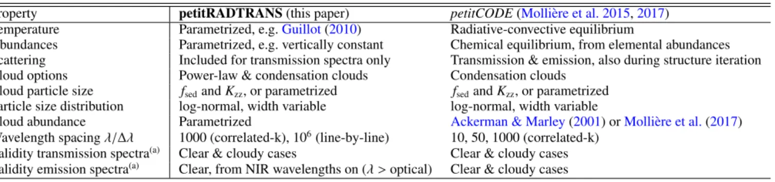
Table 1.Table summarizing and comparing the general properties ofpetitRADTRANS, the code presented in this paper, and
pe-titCODE, to whichpetitRADTRANSspectral calculations are compared in Section4.2. The fsedandKzzparameters are the
mass-averaged ratio of the cloud particle settling speed and the mixing velocity, and the atmospheric eddy diffusion coefficient, respec-tively, as described inAckerman & Marley(2001). (a):petitRADTRANSdoes not treat scattering for emission spectra, so emission spectra ofpetitRADTRANSwhere cloud scattering is expected to play an important role should be used with caution.
chemical equilibrium. Consequently, temperature profiles, abun-dance and cloud parameters are the retrievable quantities.
peti-tRADTRANS is thus different from petitCODE(Molli`ere et al.
2015, 2017), which is our model for solving for atmospheric structures and spectra self-consistently. Also see Table1for the differences in modeling philosophy between the two codes, the spectra of which will be compared in Section4.2.
Before summarizing the capabilities of petitRADTRANS, and the corresponding structure of this paper, we give a short overview of the tools and codes already publicly available:
Tau-REx (Waldmann et al. 2015a,b) is a Python radiative transfer
plus retrieval code which, similar topetitRADTRANS, allows to calculate emission and transmission spectra, at low or high reso-lution, including clouds. The code and some documentation are available on github1. TheBART code for exoplanet emission or
transmission spectral retrieval is available from github2, along
with a partial documentation, also see Section 2.2 of Blecic
et al. (2017), and Chapter 5 of Cubillos(2016). Pyrat Bayis
a Python code for synthesizing emission and transmission spec-tra, and carrying out retrievals, which is already documented3,
but not yet publicly available. The transmission spectrum part of
theCHIMERAcode (e.g.Line et al. 2013,2016, but seeBrogi &
Line 2018for its most recent description) is available on github4,
currently without documentation.HELIOS-Ris a retrieval code that was used for inferring properties of the HR 8799 planets via their emission spectra (Lavie et al. 2017). The code has been ad-vertized to be publicly available at some point5.PLATON is a
recently published Python retrieval package that calculates ex-oplanet transmission spectra (Zhang et al. 2019). It is available on github6, and now also appears to allow for the calculation of emission spectra7. ThePLATONcode is designed to maximize
computational speed, such that retrievals of transmission spectra can be carried out within minutes on a standard computer. This is done at the expense of the accuracy of the results: the opacity-sampling employed inPLATONadds white noise, making their transit depths accurate to only 100 parts per million (ppm). Due to the white-noise nature of the inaccuracies this should in first order only affect the width of their retrieved posterior
distribu-1 https://github.com/ucl-exoplanets/TauREx_public
2 https://github.com/exosports/BART
3 https://pcubillos.github.io/pyratbay/
4 https://github.com/ExoCTK/chimera/
5 https://github.com/exoclime/HELIOS-R
6 https://github.com/ideasrule/platon
7 https://platon.readthedocs.io/en/latest/
tions, and for retrievals with data of lower resolution than the intrinsic wavelength spacing of the code, opacity sampling inac-curacies are largely averaged out (Zhang et al. 2019). A detailed discussion of the effect of opacity sampling, and wavelength-averaged cross-sections, on the accuracy of spectral calculations, can be found in the recent study byGarland & Irwin(2019).
InpetitRADTRANS, spectra can be calculated at low (λ/∆λ=
1000) and high (λ/∆λ = 106) resolution, using a
correlated-k or line-by-line frameworcorrelated-k, respectively. The implementation of the radiative transfer, including the contribution functions, is described in Section 2. The high-resolution part of
petitRAD-TRANS has already been used in Molli`ere & Snellen (2018).
The opacity database, including line opacities, cloud opacities and gas quasi-continuum opacities, is described in Section 3. At low or high resolution, spectra are calculated within a few seconds, scaling linearly with the wavelength coverage.8At low resolution, this speed is lower than the fastest publicly avail-able radiative-transfer codes, for examplePLATON(Zhang et al. 2019), which takes a fraction of a second. However, as de-scribed above, the opacity sampling employed in their work adds white noise. petitRADTRANSwould be at least 16 times faster (the number of the correlated-k sub-bins is 16) if opacity sam-pling was employed. Because of the use of correlated-k,
peti-tRADTRANSlow and high-resolution spectra agree excellently,
see Section 4. In this section we also verify petitRADTRANS
by comparing to our self-consistentpetitCODE(Molli`ere et al. 2015, 2017), also using models with condensate clouds. This verification means thatpetitRADTRANSis also consistent with with theATMO(Tremblin et al. 2015) andExo-REM(Baudino
et al. 2015) codes, because petitCODE has been successfully
benchmarked against these, see Baudino et al. (2017). petit-CODE has also been used to carry out grid retrievals of self-luminous planets and brown dwarfs (Samland et al. 2017), the latter comparing well to the CHIMERA results in Line et al.
(2015). After verification, we test retrievals of synthetic JWST
emission and transmission spectra withpetitRADTRANS, carried out on a small cluster (using 30 cores), see Section5. For com-puting quantities such as the planet-to-star flux ratio, or stellar heterogeneity effects (Rackham et al. 2018), petitRADTRANS
8 For the high resolution mode this describes the computational time
also includes a library of PHOENIX (Husser et al. 2013) and
ATLAS9(Kurucz 1979,1992,1994) spectra, as described invan
Boekel et al.(2012). This library returns the stellar spectrum as
a function of the stellar effective temperature.
petitRADTRANS is available at http://gitlab.com/
mauricemolli/petitRADTRANS, and its documentation can
be found athttps://petitradtrans.readthedocs.io. Our Python retrieval implementation (see Section 5), using
peti-tRADTRANSandemcee(Foreman-Mackey et al. 2013), can be
found there as well.petitRADTRANSmakes use of the Numpy library (Oliphant 2006).
2. Code description
petitRADTRANS consists of two resolution modes. The
correlated-k mode (‘c-k’) calculates spectra making use of the correlated-k approximation (see below), at a wavelength spac-ing of λ/∆λ = 1000. The line-by-line mode (‘lbl’) calculates the radiative transfer in a line-by-line fashion, that is directly in wavelength space. The line-by-line wavelength spacing is
λ/∆λ=106.
2.1. Emission spectra
2.1.1. Radiative transfer implementation
For the calculation of the emission spectra we calculate the in-tensity along rays of different directions. For this we assume a plane-parallel atmosphere, that the atmosphere is in LTE, and neglect scattering, to speed up retrieval calculations. Neglecting scattering will mostly affect the blue part of the spectrum, and the near-infrared, if the atmospheres are cloudy, as we show in Section 4.2. Scattering is included when calculating transmis-sion spectra, see below. In a discrete-layer representation, the arising intensity in a plane-parallel atmosphere can be written as
¯
Itop=B¯(Tbot) ¯Tatmo+1
2
NL−1 X
i=0
h¯
B(Ti)+B¯(Ti+1)i T¯i−T¯i+1, (1)
see, e.g., Section 6.3.1 inMolli`ere(2017). HereNLis the num-ber of atmospheric layers and the bar on top of a symbol (e.g.
¯
B) denotes the wavelength average of that quantity, within the correlated-k spectral bin of interest.Bdenotes the Planck func-tion, and here we used that it is roughly constant across one of these bins, and replaced it with its mean value within the bin.T denotes the atmospheric transmission from a given layer to the top of the atmosphere, and Tatmo is the transmission from the
bottom to the top of the atmosphere. Equation 1is equivalent to Equation 13 inIrwin et al. (2008). For the line-by-line cal-culations at high resolution, this equation is simply evaluated at every wavelength step.
Using the correlated-k assumption, and further making the standard assumption that the opacity distribution functions be-tween given molecular species are uncorrelated (e.g. Lacis &
Oinas 1991;Fu & Liou 1992), we can write the transmission
from a layeri, at pressurePi, to the top of the atmosphere, at
pressureP=0, as
¯ Ti=
Nspec
Y
j=1
Ng
X
l=0
exp −
Z Pi
0
Xjκl j
aµ dP
!
∆gl
=
Nspec
Y
j=1
¯
Tji, (2)
see, e.g., Appendix A.5 in Molli`ere (2017). Here Nspec is the number of species,Ng the number of the Gaussian quadrature
points in g-space (whereg is the coordinate of the cumulative opacity distribution function), X the mass fraction of a given species in a given atmospheric layer, athe gravitational accel-eration within the atmosphere, and κ a given species’ opacity. The angleϑbetween the atmospheric normal and the ray is ac-counted for through the 1/µ = 1/cosϑin the exponential. In particular, from Equation1one sees that if emission is the only process of interest, and the atmospheric temperature structure is known, only the atmospheric transmissions and Planck func-tions need to be computed. The transmission of given layersi
to the top of the atmosphere themselves are the products of the transmissions ¯Tjiof the atmosphere’s individual opacity species
j. This means that the numerically expensive computation of a combined correlated-k opacity table is not necessary. This allows for a fast correlated-k application in retrieval calculations.
For the line-by-line calculations at high resolution we do not employ this ‘product of transmissions’ method. Rather, we cal-culate the total opacity by simply adding opacities of all opacity species in every spectral bin, and then calculate the transmission of the atmosphere. This conserves the wavelength correlation be-tween the opacities of all species, and is hence not subject to the classical correlated-k assumption of uncorrelated opacity distri-butions.
We solve the radiative transfer on a 3-point Gaussian grid for the angleµ=cosϑbetween rays and the atmospheric normal, for which we found only small differences when comparing to the 20-point Gaussian grid used inpetitCODE, see Section4. The flux is then calculated as
F=2π
Nµ X
k=1
µkI¯top(µk)∆µk, (3)
which follows fromF=2πR01µI(µ)dµ.
2.1.2. Contribution function implementation
The emission contribution function quantifies the relative impor-tance (contribution) of the emission in a given layer to the total atmospheric flux. Using equations1and3, one can see that the relative contribution of a given layer, at spatial coordinatei+1/2, to the total flux is
Ciem+1/2 =
PNµ
k=1c
i+1/2(µ
k)µk∆µk
PNµ
l=1
h
2 ¯B(Tbot) ¯Tatmo(µl)+PNL−1
j=1 cj+1/2(µl)
i
µl∆µl,
(4) where
ci+1/2(µk)=hB¯(Ti)+B¯(Ti+1)i hT¯i(µk)−T¯i+1(µk)i. (5)
These equations are evaluated in petitRADTRANS when the emission contribution function is calculated.
2.2. Transmission spectra
2.2.1. Radiative transfer implementation
r1 P1
r2
r3
…
r4
rN -1
rN
P2
P3
…
P4
PN -1
PN r3
r2 r1
𝜌4, 𝜅4 𝜌1, 𝜅1 𝜌2, 𝜅2 𝜌3, 𝜅3
L L
L L
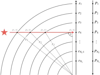
Fig. 1. Geometry of the transmission problem using the same
notation as in Section2.2. The red line shows a grazing light ray as it passes through the planetary atmosphere.
be specified. The optical depth of a ray of light, grazing the at-mosphere at impact parameterriabove the planetary center, can then be written as
τi=
i−1 X
j=1
κjρj+κj+1ρj+1
q
r2
j−r
2
i −
q
r2
j+1−r
2 i
, (6)
where ρj is the mass density of the atmospheric layer at
ra-diusrj. The geometry of the transmission problem is sketched in Figure 1. The factor 1/2 of the integrand approximation (κjρj+κj+1ρj+1)/2 cancels with the factor 2 in front of the
inte-gral, for grazing rays approaching and receding from the point of closest approach to the planet’s center.
The effective area of the planet is calculated as
A=2π
Z Rpl
0
r(1− T)dr, (7)
whereT =e−τ again denotes the transmission of light through
the atmosphere, this time in grazing geometry. As before it is possible to write the transmission as the product of the individ-ual species’ transmissions, greatly speeding up the correlated-k treatment in the process.
Again, for the line-by-line calculations at high resolution we do not employ this ‘product of transmissions’ method. Rather, we calculate the total opacity by simply adding opacities of all opacity species in every spectral bin, and then calculate the trans-mission of the atmosphere.
InpetitRADTRANS, Equation7is solved numerically,
start-ing from the bottom of the atmosphere, assumstart-ing that the planet is opaque at all wavelengths at the lowest altitude.
2.2.2. Contribution function implementation
Transmission contribution functions can be defined in multiple ways, for example by determining the pressure for which a cer-tain optical depth is reached, in transit geometry. We suggest and use different method here, which quantitatively measures the im-portance of a given layer when forming the transmission spec-trum.
For a given layeri, the transmission contribution at a given wavelength is calculated using
Citr= R
2
nom−R2(κi=0)
PNL
j=1
h
R2nom−R2(κj=0)
i , (8)
whereRnomis the planet’s nominal transmission radius at a given
wavelength, andR(κi=0) is the transmission radius one obtains when setting the opacity in theith layer to zero, and recalculating the transmission spectrum. Squared radii are used here, because transmission spectra measure the flux decrease of the star as it is transited by its planet, which is proportional to the planet’s area. Calculating the transmission function in the way presented here has the advantage that only those layers which can actually change the transmission radius are assigned a large contribution. High altitude layers will not contribute strongly, because they are optically thin, whereas low altitude layers will be negligible because they are hidden from view by the overlying layers.
3. Opacities
Below we describe the references for the various opacity sources available withinpetitRADTRANS, which encompass molecular and atomic line opacities, cloud opacities (absorption and scat-tering), Rayleigh scattering cross-sections, and quasi-continuum opacities (collision induced absorption, H−bound-free (b-f) and free-free (f-f) absorption). The opacities are published together with the code.
3.1. Line opacities
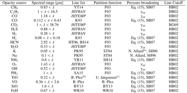
petitRADTRANSallows to include the line opacities of Na, K,
CH4, C2H2, CO, CO2, H2S, H2, HCN, H2O, NH3, O3, OH,
PH3, TiO, VO, SiO and FeH. High temperature linelists are
used when available, see Table 2 for the references. For all molecules, except for CO and TiO, only the main isotopologue opacities are used in the low-resolution mode. For CO and TiO all isotopologues where included, at telluric occurrence rates, because here we found that they add a signigcant amount of opacity already at low resolution. In the high-resolution mode, also secondary isotopologues are available, for example for H2O,
CH4 and CO. See the code documentation website athttps:
//petitradtrans.readthedocs.iofor the up-to-date list of
high-resolution species.
The documentation website also contains a short tutorial of
theExoCrosscode (Yurchenko et al. 2018), and how to convert
its resulting Exomolopacity calculations for use in
petitRAD-TRANS. This allows thepetitRADTRANSuser to calculate line
opacities of additional species, for the low and high resolution modes.
Pressure broadening is included either by using the air broad-ening coefficients ofHITRAN/HITEMP (Rothman et al. 2010,
2013), or Equation 15 ofSharp & Burrows(2007). Using the air broadening coefficientsγairmay sound like a stretch for the of-ten H2/He-dominated exoplanet atmospheres. However,
Gharib-Nezhad & Line (2018) have shown that the ratio between air
and H2/He broadening ranges from values of 1 to 2 (see their Table 1). Nonetheless, we plan to include H2/He broadening in future versions of the opacity database.Gharib-Nezhad & Line
(2018) also showed that care must be taken if the atmospheres are strongly enriched: self-broadening of water then becomes much stronger than that of H2/He, or air.
For all molecules, except for CO2, a line cutoffis included
Opacity source Spectral range [µm] Line list Partition function Pressure broadening Line Cutoff
CH4 0.83< λ YT14 F03 Eq. (15), SB07 HB02
C2H2 1< λ <16.5 HITRAN F03 γair HB02
CO 1.18< λ HITEMP F03 γair HB02
CO 0.112< λ <0.43 K93 F03 Eq. (15), SB07 HB02
CO2 1< λ <38.76 HITEMP F03 γair BG69
H2S 0.88< λ HITRAN F03 γair HB02
H2 0.28< λ HITRAN F03 γair HB02
H2 0.08< λ <0.18 K93 F03 Eq. (15), SB07 HB02
HCN 2.92< λ HT06, BS14 F03 Eq. (15), SB07 HB02
H2O 0.33< λ HITEMP F03 γair HB02
K 0.05< λ PK95 ST84 N. Allard(a), SH96 HB02
Na 0.1< λ PK95 ST84 N. Allard, SH96 HB02
NH3 0.8< λ YB11 SH14 Eq. (15), SB07 HB02
O3 1.43< λ HITRAN F03 γair HB02
OH 0.52< λ HITEMP F03 γair HB02
PH3 1< λ SA15 F03 Eq. (15), SB07 HB02
TiO 0.32< λ B. Plez(b) U. Jørgensen(c) Eq. (15), SB07 HB02
VO 0.36< λ <2.6 B. Plez B. Plez Eq. (15), SB07 HB02
SiO 1.6< λ BY13 BY13 Eq. (15), SB07 HB02
FeH 0.67< λ WR10 WR10 Eq. (15), SB07 HB02
Table 2. References for the atomic and molecular opacities available for use in petitRADTRANS. Reference codes: HITEMP
Rothman et al. (2010), HITRAN: Rothman et al. (2013), SB07: Sharp & Burrows (2007), F03: Fischer et al. (2003), ST84:
Sauval & Tatum (1984), K93: Kurucz (1993), YT14: Yurchenko & Tennyson (2014), YB11:Yurchenko et al. (2011), SH96:
Schweitzer et al. (1996), SH14:Sousa-Silva et al. (2014), SA15: Sousa-Silva et al.(2015), HT06: Harris et al. (2006), BS14:
Barber et al.(2014), PK95:Piskunov et al.(1995), HB02:Hartmann et al.(2002), BG69:Burch et al.(1969), BY13:Barton et al.
(2013), WR10:Wende et al.(2010), (a): line profile available athttp://mygepi.obspm.fr/˜allard/alkalitables.html, (b): line list available at http://www.pages-perso-bertrand-plez.univ-montp2.fr/, (c): partition function retrievable from
http://www.astro.ku.dk/˜uffegj/scan/scan_tio.pdf. If names of researchers are given without a footnote, then the data
have been obtained from private communication. For all molecules, except for CO and TiO, only the main isotopologue opacities are used in the low resolution mode. At high resolution also secondary isotopologues are available for some species, see the docu-mentation athttps://petitradtrans.readthedocs.iofor an up-to-date list. The documentation website also contains a short tutorial of theExoCrosscode (Yurchenko et al. 2018), and how to convert its resultingExomolopacity calculations for use in
peti-tRADTRANS. This allows thepetitRADTRANSuser to calculate line opacities of additional species, for the low and high resolution
modes.
Quasi-continuum Reference Clouds Reference Rayleigh Reference
H2–H2CIA BR, RG12 Al2O3 Koike et al.(1995) H2 Dalgarno & Williams(1962)
H2–He CIA BR, RG12 H2O (ice) Smith et al.(1994) He Chan & Dalgarno(1965)
H−
bound-free Gray(2008) Fe Henning & Stognienko(1996) CO Sneep & Ubachs(2005)
H−
free-free Gray(2008) KCl Palik(2012) CO2 Sneep & Ubachs(2005)
MgAl2O4 Palik(2012) CH4 Sneep & Ubachs(2005)
MgSiO3 Scott & Duley(1996), H2O Harvey et al.(1998)
Jaeger et al.(1998)
Mg2SiO4 Servoin & Piriou(1973) O2 Thalman et al.(2014,2017)
Na2S Morley et al.(2012) N2 Thalman et al.(2014,2017)
SiC P´egouri´e(1988)
Table 3. Quasi-continuum, Rayleigh and cloud opacities available inpetitRADTRANS. References BR stand for: Borysow et al.
(1988,1989);Borysow & Frommhold(1989);Borysow et al.(2001);Borysow(2002), while RG12 stands forRichard et al.(2012),
and the references therein.
broadened by H2(Hartmann et al. 2002). For CO2, the line wing
decrease is modeled using a fit to the CO2 measurements by
Burch et al.(1969). This fit was obtained from Bruno B´ezard
(private communication).
The line opacities are calculated from 110 nm to 250µm, 80-3000 K, and 10−6-103bar. In the high-resolution mode (λ/∆λ=
106), the opacities only range from 0.3 to 28 micron. The
pres-sure and temperature points are spaced equidistantly in log-space on a 10×13 point grid. If aP-Tstructure is defined that goes out-side of thePandT range mentioned here,petitRADTRANSwill use the opacities at the boundary of the grid. Given this upper temperature boundary,petitRADTRANScan calculate the fluxes of terrestrial planets, super-Earths, Neptunes, and hot Jupiters,
if their atmospheres are hydrogen-dominated. Higher tempera-ture points and species will be added in the futempera-ture, increasing the temperature resolution and range of the existing grid, and allowing to also model the class of ultra hot-Jupiters, with equi-librium temperatures Teq & 2000 K (see, e.g.,Arcangeli et al.
2018;Lothringer et al. 2018;Lothringer & Barman 2019). Thus,
for now, the results of spectral calculations and retrievals of ul-trahot Jupiters must be treated very carefully. This is because the spectrally active regions can reach temperatures larger than 3000 K for planets of equilibrium temperatures of about 2000 K and above.
100 101 Wavelength (micron)
0 1 2 3 4 5 6 7
Surface
flux
Fν
(10
−
6erg
cm
−
2s
−
1Hz
−
1)
Clear TrES-4b,petitRADTRANS radiative transfer cross-verification
petitRADTRANS, high resolution (‘lbl’ mode)
petitRADTRANS, high resolution, rebinned to low resolution
petitRADTRANS, low resolution (‘c-k’ mode)
100 101
−10 0 10
Relativ
e
deviation
(%)
petitRADTRANS low resolution - high resolution (rebinned)
100 101
Wavelength (micron) 1.80
1.85 1.90 1.95 2.00 2.05 2.10 2.15 2.20
T
ransmission
radius
(RX
)
petitRADTRANS, high resolution (‘lbl’ mode)
petitRADTRANS, high resolution, rebinned to low resolution
petitRADTRANS, low resolution (‘c-k’ mode)
100 101
−0.25 0.00 0.25
Relativ
e
deviation
(%)
petitRADTRANS low resolution - high resolution (rebinned)
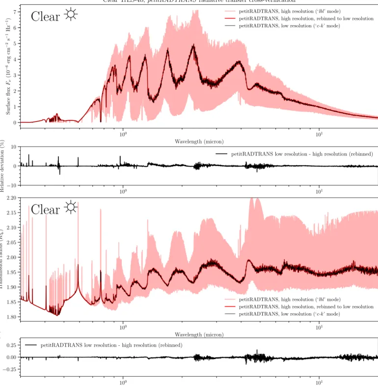
Fig. 2.Radiative transfer verification ofpetitRADTRANS. Theuppermost panelshows the comparison between the emission
spec-tra of a clear TrES-4b-like atmosphere, calculated with petitRADTRANSin high-resolution (‘lbl‘) mode (light red), and in low-resolution (‘c-k‘) mode (black, thin line). The red line denotes the re-binned high-resolution spectrum. The panel below shows the residuals between the two modes. Thesecond lowest panelshows the comparison between the transmission spectra of the same atmosphere, for both modes. Thelowest panelshows the residuals between the two modes, for the transmission spectrum.
Gaussian quadrature grid is used for thegcoordinate of the cu-mulative opacity distribution function. This g-grid is separated into an 8-point grid ranging fromg=0 tog=0.9 and a second 8-point grid ranging fromg=0.9 tog=1. At high resolution the wavelength binning of the line-by-line opacities isλ/∆λ=106.
3.2. Rayleigh Scattering
The Rayleigh cross-sections of the following atoms and molecules can be included inpetitRADTRANScalculations: H2,
He, CO, CO2, CH4, H2O, O2 and N2. See the right column of
3.3. Cloud opacities
petitRADTRANS allows for including clouds in four different
ways:
1. By defining a gray cloud deck pressure, below which the at-mosphere cannot be probed (effectively we add an absorption opacityκ=1099cm2/g at all wavelengths, there and below).
This can also be used to implement a maximum visible pres-sure in transmission spectra, due to atmospheric diffraction, see, for example, Equation 15 inRobinson et al.(2017). 2. By scaling the value of the Rayleigh scattering cross-section
of the gas
κ= f ·κRayleigh(λ), (9)
where f is the scaling factor and κRayleigh is the Rayleigh
opacity of the atmospheric gas. In this case the Rayleigh scattering opacity will hence be f times larger.
3. By introducing a scattering cross-section with two free pa-rametersκ0andγ,
κ=κ0
λ
λ0
!γ
, (10)
whereκ0 is the opacity at 0.35µm, in units of cm2/g. This is equivalent to the parametrization used in, e.g.,MacDonald
& Madhusudhan(2017).
4. By including solid Al2O3, H2O, Fe, KCl, MgAl2O4,
MgSiO3, Mg2SiO4 or Na2S clouds, for which the optical
constants given in the middle column of Table3 are used. For this mode, the altitude-dependent cloud mass fraction, mean radius of the particles, and the width of the log-normal particle size distribution, need to be specified. The particle radius can also be calculated by specifying the atmospheric eddy diffusion coefficientKzzand settling parameter fsed, as described and defined inAckerman & Marley(2001).
The four cloud modes described above can be used indepen-dently, but also in combination. For emission spectra only the absorption component of the cloud options listed above will be used, if present (that is, options 1 and 4). It is also possible to test for the importance of scattering by adding the scattering opacity as an absorption opacity.
The cloud opacities of the species listed in Table3are calcu-lated assuming either homogeneous and spherical, or irregularly shaped cloud particles. Comparing spectra using these different cloud opacity treatments could allow for the distinction between particle shapes. This holds for particles of small enough grain sizes (. 1 µm), for which the resonance features of the cloud species are most clearly visible (Min et al. 2005).
The opacity of the irregularly shaped cloud particles is ap-proximated by taking the opacities obtained for a Distribution of Hollow Spheres (DHS). For spherical and DHS cloud particles, the opacities were calculated with the code ofMin et al.(2005), which also uses software reported inToon & Ackerman(1981). Spherical particle cross-section are obtained from Mie theory, while an extended Mie formulation is assumed in the DHS case. For DHS, a porosity ofP=0.25 (as inWoitke et al. 2016) and an irregularity parameter fmax = 0.8, as defined in Min et al.
(2005), are used.
The opacities were calculated for particles of sizes between 1 nm and 10 cm. If thepetitRADTRANSuser requests opacities for particles with sizes outside this range, the returned opacity for the corresponding cloud species will be zero.9
9 It is also possible to request cloud opacities for a log-normal size
distribution. In this case all size ranges outside of the 1 nm to 10 cm interval will not contribute to the total opacity.
3.4. Other continuum opacities
petitRADTRANSallows to include H2-H2 and H2-He Collision
Induced Absorption (CIA) cross-sections, as well as the bound-free and bound-free-bound-free absorption of H–. See the left column of Table
3for the references.
4. Code verification
In Section 4.1 we compare the low-resolution (‘c-k’) mode to the high-resolution (‘lbl’) mode of petitRADTRANS. We hence verify our correlated-k (at low resolution) and line-by-line (at high resolution) implementation, because binned high-resolution spectra should be equal to the correlated-k results at lower resolution.
In Section4.2we compare the low resolution (‘c-k’) mode
of petitRADTRANSwith the radiative transfer calculations
ob-tained from petitCODE. petitCODE is a 1-d, self-consistent atmospheric code, solving for the atmospheric structure in radiative-convective and chemical equilibrium (Molli`ere et al.
2015, 2017). petitCODE radiative transfer includes scattering,
and makes use of the correlated-k assumption. InBaudino et al.
(2017), it has been successfully benchmarked with theATMO
(Tremblin et al. 2015) and Exo-REM (Baudino et al. 2015)
codes. Moreover,petitCODEresults have themselves been veri-fied by comparing to line-by-line, high-resolution (λ/∆λ=106)
calculations, which where binned to petitCODE’s wavelength sampling (Molli`ere et al. 2015). See Table 1for a comparison between the modeling approaches inpetitRADTRANSand
petit-CODE.
For the comparisons presented here, the input atmospheric temperature and abundance structures where obtained from a self-consistent petitCODE solution, assuming T∗ = 6295 K,
R∗ =1.831 R,d =0.0516 au,Tint =100 K, MP =0.494 MX, RP = 1.838 RX. We assumed a planetary metallicity of [Fe/H]
=1.1 and a solar C/O ratio (0.55). We assumed a dayside redis-tribution of the stellar flux. These parameters where taken from our TrES-4b model inMolli`ere et al.(2017).
4.1. Comparing the high (‘lbl’) and low (‘c-k’) resolution modes
Figure2shows the comparison between the high (‘lbl’) and low (‘c-k’) resolution modes ofpetitRADTRANS, for the clear TrES-4b-like atmosphere. One can see that both emission and trans-mission spectra agree very well, with the errors scattering around zero, and in the low, single-digit percentage range, as usually found for correlated-k implementations (see, e.g.,Lacis & Oinas
1991;Fu & Liou 1992;Molli`ere et al. 2015).
4.2. ComparingpetitRADTRANStopetitCODE
4.2.1. Clear atmospheres
The upper panel of Figure3shows a comparison between
petit-CODEandpetitRADTRANSemission spectra. ThepetitCODE
emission spectra are plotted with and without scattering. The
petitRADTRANS spectra do not include scattering. The diff
100 101 Wavelength (micron)
0 1 2 3 4 5
Surface
flux
Fν
(10
−
6erg
cm
−
2s
−
1Hz
−
1)
Clear TrES-4b,petitRADTRANS–petitCODE comparison
petitCODE, with scattering petitCODE, without scattering petitRADTRANS
100 101
−10 0 10
Relativ
e
deviation
(%)
petitRADTRANS - petitCODE
petitRADTRANS - petitCODE (without scattering)
100 101
Wavelength (micron) 1.800
1.825 1.850 1.875 1.900 1.925 1.950 1.975 2.000
T
ransmission
radius
(RX
)
petitCODE
petitRADTRANS, constant gravity petitRADTRANS, variable gravity
100 101
−0.25 0.00 0.25
Relativ
e
deviation
(%)
petitRADTRANS (constant gravity) - petitCODE
petitRADTRANS (constant gravity) - petitRADTRANS (variable gravity)
Fig. 3.Radiative transfer verification ofpetitRADTRANS. Theuppermost panelshows the comparison between the emission spectra
of a clear TrES-4b-like atmosphere, calculated withpetitRADTRANS(red),petitCODEwithout scattering (black) andpetitCODE
with scattering (gray). The agreement between petitCODE (with scattering) andpetitRADTRANSbreaks down for wavelengths below 0.5µm, because Rayleigh scattering becomes important (petitRADTRANSdoes not include scattering for emission spectra).
The second lowest panelshows the comparison between the transmission spectra of the same atmosphere, calculated with
peti-tRADTRANS when assuming a constant surface gravity (red), when assuming a variable gravity (purple), and with petitCODE,
which assumes a constant gravity (black). Here, the constant gravity cases agree well also in the short wavelength range, because scattering is included for transmission spectra inpetitRADTRANS. The comparison between the constant and variable gravity cases
ofpetitRADTRANShighlights the effect of varying gravity on the resulting spectra. The panels below the emission and transmission
spectra show the relative deviation of thepetitRADTRANScalculations, which are shown as red lines in the spectral plots, to the other cases.
andpetitRADTRANS. We checked multiple times and are certain
that we use the same CO opacities in both codes. Differences in the numerical radiative transfer treatment between of
petitRAD-TRANSandpetitCODEmay be responsible for these small
dif-ferences, but prove difficult to identify. We note thatpetitCODE
100 101 Wavelength (micron)
0 1 2 3 4
Surface
flux
Fν
(10
−
6erg
cm
−
2s
−
1Hz
−
1)
Cloudy TrES-4b,petitRADTRANS–petitCODEcomparison
petitCODE, with scattering petitCODE, without scattering petitRADTRANS
100 101
−10 0 10
Relativ
e
deviation
(%)
petitRADTRANS - petitCODE
petitRADTRANS - petitCODE (without scattering)
100 101
Wavelength (micron) 1.88
1.90 1.92 1.94 1.96 1.98 2.00 2.02 2.04
T
ransmission
radius
(RX
)
petitCODE
petitRADTRANS, constant gravity petitRADTRANS, variable gravity
100 101
−0.25 0.00 0.25
Relativ
e
deviation
(%)
petitRADTRANS (constant gravity) - petitCODE
petitRADTRANS (constant gravity) - petitRADTRANS (variable gravity)
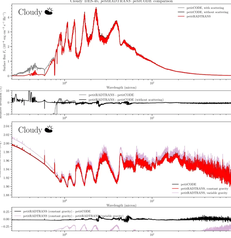
Fig. 4.Same as Figure3, but for the cloudy case.
coordinate (Molli`ere et al. 2015), whereaspetitRADTRANSuses 16 points (see Section3.1). However, we have verified in Section
4.1that the correlated-k implementation ofpetitRADTRANS re-produces the line-by-line results very accurately. Moreover, the differences in solving the radiative transfer equation for emis-sion spectra are not a likely candidate (Feautrier method in petit-CODE, Equation1inpetitRADTRANS), because the same wave-lengths show small systematic differences for the transmission spectra, see discussion below. These differences could point to a somewhat smaller accuracy of thepetitCODEopacity treatment, when compared withpetitRADTRANS. InpetitCODEthe opac-ities are combined to yield the correlated-k opacity table for the
full gas mixture, which is needed for calculating the atmospheric temperature structure, and scattering source function. For this combination we assume that the individual species’ opacities are not correlated in wavelength space. The same mathemati-cal assumption pertains to the ‘multiplication of transmissions’ treatment ofpetitRADTRANS, but it may result in a different be-havior, in terms of numerical errors.
Hot Jupiters typically have planet-to-star contrasts between 10−3 and 10−4. Flux differences of up to 4 %, as we obtain for
thepetitRADTRANS–petitCODEcomparison here, hence lead to
Because the model considered here is cloud-free, scattering does not play an important role for the majority of the spectrum. Only forλ <0.5µm significant differences betweenpetitCODE
(with scattering, here leading to reflection of the stellar light)
andpetitRADTRANS(without scattering) start to appear (up to
∼90 % relative deviation). We note that not much flux is escap-ing from the planetary atmosphere at such small wavelengths. Hence we expect that petitRADTRANScan calculate emission spectra of cloud-free hot Jupiters within the wavelength range of the upcomingJWST(Beichman et al. 2014).
There also appear to be some larger differences in the wings of the alkali lines of secondary importance (at ∼0.4 micron), which do not occur for the transmission spectrum implemen-tation, see below. Here we again tested for various effects that could likely explain this difference. We could rule out, for ex-ample, that it is the smaller number of ray angles used for calcu-lating the radiation field (20 inpetitCODEcompared to 3 in
pe-titRADTRANS), because using as many angles as inpetitCODE
did not change the results.
In the two lower panels of Figure 3 the comparison of the transmission spectra of petitRADTRANS and petitCODE
is shown. InpetitRADTRANS transmission spectra the surface gravity is varying as a function of altitude, with anr−2 depen-dence, whereris the planet’s radial coordinate. In contrast,
pe-titCODE is a code which solves for the atmospheric structure
assuming a plane-parallel atmosphere, using the pressure as its vertical coordinate. For this, the variation of the surface grav-ity is neglected, also during the calculation of the petitCODE
transmission spectra. We hence show two different
petitRAD-TRANScalculations when comparingpetitCODEand
petitRAD-TRANSspectra: one with varying surface gravity (nominal) and
one where the surface gravity is constant. The reference pres-sure for the transmission spectra was chosen to beP0=0.01 bar
forpetitCODEandpetitRADTRANS, such thatr(P0) =RPand
g(r(P0))=−GMP/R2
P.
As can be seen, the agreement betweenpetitCODEand
pe-titRADTRANS(with constant gravity) is of similar quality as in
the emission case. The optical part (λ <0.5µm) is reproduced better than in the emission case, because photon extinction due to scattering is included in thepetitRADTRANScalculations for transmission spectra.
The difference of including the effect of varying gravity is visible as well, when comparing the constant and variable gravity calculations ofpetitRADTRANS: in wavelength regions where the opacity is large, smaller pressures than the reference pressure are probed. Here the deviation from the constant surface gravity assumption is most visible.
4.2.2. Cloudy atmospheres
In this section we discuss the comparison between
petitRAD-TRANS andpetitCODE, for cloudy atmospheres. We used the
same atmospheric setup for petitCODE as for the clear case, but self-consistently included clouds of Na2S, KCl, Mg2SiO4,
and MgAl2O4 in the atmospheric structure iteration of petit-CODE. For this we used Cloud Model 6, as defined in Table 2
ofMolli`ere et al.(2017), which corresponds to clouds of single
particles size, with particle radii of 0.08µm. This particle size was chosen because it highlights how small silicate particles can lead both to strong (Rayleigh) scattering in the optical, as well as silicate resonance features in the mid-infradred. The cloud loca-tion in the atmosphere is coupled to equilibrium chemistry, that is the clouds can only exist in regions where the condensates do not evaporate. The cloud mass fraction is equal to the
con-densates’ mass fraction in chemical equilibrium, but is capped at a maximum value of 3×10⁻⁴·Z
P, whereZP is the planet’s
metal mass fraction. This upper value can thus be thought of as effectively parametrizing the particle settling strength. The value chosen here represents and intermediate choice for the cloud set-tling strength, also see Table 2 inMolli`ere et al.(2017). For the calculations shown here, irregularly shaped, crystalline particles were assumed, for which we made use of the DHS opacities (see Section3.3).
The corresponding spectra for the cloudy case are shown in Figure4. For the emission case we again see a good agreement betweenpetitCODE(including scattering) andpetitRADTRANS, with the difference that scattering (mainly leading to the reflec-tion of stellar light) now already becomes important at larger wavelengths (forλ <0.8µm), due to the added haze-like scat-tering of the clouds. It is noteworthy that the agreement at longer wavelengths is very good, although the transmission spectrum of the planet shows the significant impact of clouds (cf. clear transmission spectrum in Figure3), also the 10-micron feature of Mg2SiO4 (e.g.Wakeford & Sing 2015;Molli`ere et al. 2017)
is visible. This difference in the visibility of clouds, when com-paring emission and transmission spectra, can be explained by the different geometries when probing the atmosphere in trans-mission (Fortney 2005). For transmission, we again find a good agreement betweenpetitCODEandpetitRADTRANS.
For completeness, we also show a comparison to a model with even thicker clouds, see Figure A.1in Appendix A, cor-responding to Cloud Model 5 inMolli`ere et al.(2017). In this model the cloud mass fraction is only capped at 10−2·ZP. While
we again find a good agreement between the transmission spec-tra ofpetitCODE andpetitRADTRANS, this is not the case for emission spectra, out to wavelengths of 4.5µm, due to the strong scattering of light by cloud particles (resulting in both reflec-tion of stellar light and scattering of light originating within the planet atmosphere).
5. Retrieval examples, low resolution (‘c-k’) mode
In this section we show an exemplary use ofpetitRADTRANSfor a retrieval analysis. Here, we focus on simple, clear atmosphere scenarios.
5.1. Retrieval setup
petitRADTRANS is a radiative transfer code for Python. That
means that the retrieval needs to be implemented by the user, with Python tools such as the MCMC implementation emcee
(Foreman-Mackey et al. 2013), or the nested sampling
imple-mentationPyMultiNest (Buchner et al. 2014). In what follows below, we will construct a simple retrieval example using em-cee. This example setup is also published and documented in the manual ofpetitRADTRANS. Users ofpetitRADTRANSmay use this as a starting point for their own retrievals, or construct independent setups themselves.
The model of the retrieval example shown here is defined by the parameters listed in Table4. Note that not all of these are necessarily free parameters. For example, below the retrieval of a transiting planet is studied, for which the planetary mass MP,
as well as a white-light radiusRwl, is known. One can thus fix
g=GMP/R2PandRP=Rwl, leaving the reference pressureP0as
a free parameter, to be found by the retrieval.
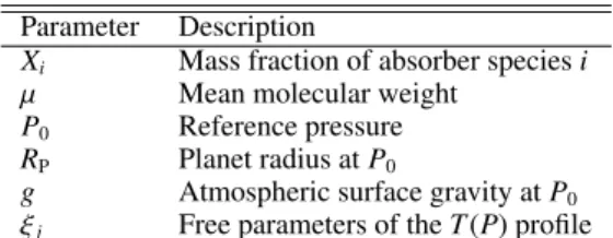
cal-Parameter Description
Xi Mass fraction of absorber speciesi
µ Mean molecular weight
P0 Reference pressure
RP Planet radius atP0
g Atmospheric surface gravity atP0
ξj Free parameters of theT(P) profile
Table 4.Parameters of the retrieval model used in this study. Not
all parameters are necessarily free parameters, see Section5.1.
Abundances Value Parameter Value
XCH4 7.71×10⁻⁹ P0 0.01 bar
XCO 5.52×10⁻³ RP 1.84 R
X
XH2O 2.46×10⁻³ g 380 cm s−2
XH2S 2.40×10⁻⁴ α(i.e.ξ1) 0.5
XK 1.52×10⁻⁶ Ptrans(i.e.ξ2) 0.001 bar
XNH3 3.80×10⁻⁸ γ(i.e.ξ3) 0.4
XNa 2.46×10⁻⁵ δ(i.e.ξ4) 10−5bar−1
XCO2 8.48×10⁻⁷ Tint(i.e.ξ5) 600 K
Teq(i.e.ξ6) 1900 K
Instrument Noise floor T∗ 6295 K
NIRISS SOSS 20 ppm R∗ 1.81 R
NIRSpec G395M 75 ppm K 10.33 mag
MIRI LRS 40 ppm ttrans 3.658 h
fbase 1
Table 5.Parameters for generating the clear TrES-4b-like model
(top) and synthetic observations (bottom). fbasedenotes the ratio of the out-of-transit and the in-transit observing time.
culating
XH and He =1−
Nmetals X
i=1
Xi, (11)
whereNmetalsis the number of metal species (all absorbers except H2and He), and using this to calculate
XH2=0.75·XH and He (12)
and
XHe=0.25·XH and He. (13)
This assumes a gas of approximately primordial composition. Molecules such as H2O are counted to belong to the metals, even
though they also contain hydrogen.
The mean molecular weightµis calculated through
1
µ =
Nspecies
X
i=1
Xi
µi
, (14)
whereNspecies =Nmetals+2, to account for H2and He. In this
ex-ample we hence assume that there are no non-absorbing chemi-cal species that carry a significant amount of mass. We note that the mean molecular weight in general should not include con-densed species, because they are not sufficiently coupled to the atmospheric gas, seeBaudino et al.(2017).
The temperature parametrization is given by
T(P)=
*
TGuillot(P)· 1−
α
1+P/Ptrans
!+
P
, (15)
with
TGuillot(P)=
3Tint4
4 2 3+δP
! +
3T4 eq
4
2 3+
1
γ√3+
γ
√ 3
− 1
γ√3
e
−γδ√3P
, (16)
which is the Guillot (2010) temperature model. In the Guillot
(2010) model the optical depth is defined as τ = PκIR/g. We defined the new parameterδ=κIR/g, such thatτ=δ·P. ThehiP
denotes a boxcar smoothing, carried out over a log(P)-width of 1.25 dex. The temperature model thus has six free parameters, namely ξ1 = α,ξ2 = Ptrans, ξ3 = γ, ξ4 = δ,ξ5 = Tint, and
ξ6=Teq.
The second term on the RHS of Equation15was introduced to allow the upper part of the atmosphere do develop a non-isothermal behavior at high altitudes, i.e. low pressures. This alleviates that the Guillot (2010) temperature model without this additional term will always lead to isothermal atmospheres at high altitudes, because it assumes a (double-)gray opacity. This is not the case for non-gray atmospheric models, (see, e.g.,
Molli`ere et al. 2015, Figure 5). The reason for this is discussed
in Chapter 6.4.2 ofMolli`ere(2017).
We have found this temperature model to be sufficiently flex-ible when fitting it to a diverse set of self-consistent temperature profiles (clear, cloudy, with and without inversions), see Figure 6.2 inMolli`ere(2017).
5.2. Retrieval of synthetic spectra generated with petitRADTRANS
In this section the results of retrieving an atmospheric structure
withpetitRADTRANSare shown. For the input spectrum to be
re-trieved, we created synthetic observations of apetitRADTRANS
spectrum, using parameters motivated by the exoplanet TrES-4b. TrES-4b should be an excellent target forJWST, likely being in the temperature range to probe the cloud properties of hot con-densates species such as silicates (Molli`ere et al. 2017). For the clear atmosphere retrieved here, the input parameters as reported in Table 5(upper part) were used. The resulting effective tem-perature of the synthetic emission spectrum is 1789 K, which is close to equilibrium temperature value of this planet, 1795 K
(Sozzetti et al. 2015).
We produced single transit/eclipse synthetic observations of
JWST’sNIRISS SOSS,NIRSpec G395M, andMIRI LRSmodes
using the PandExotool (Batalha et al. 2017). For this we used the parameters given in the lower part of Table5. The saturation level was assumed to be 80 % of the full well capacity for all in-strument modes. For the stellar spectrum necessary for calculat-ing the planet-to-star contrast we used the library ofPHOENIX
(Husser et al. 2013) andATLAS9 (Kurucz 1979, 1992, 1994)
spectra that is part of petitRADTRANS. Here, the stellar flux is returned as a function of the stellar effective temperature, using the model grid fromvan Boekel et al.(2012).
5.2.1. Emission spectra
2.5 0.0
CO = -1.41+0.88 0.89 2.5 0.0 4 2 H2 O 4 2
H2O = -2.45+0.610.52
2.5 0.0 7.5 5.0 2.5 CH 4
4 2 7.5 5.0 2.5
CH4= -6.37+1.09 2.39 2.5 0.0 7.5 5.0 2.5 NH 3
4 2 7.5 5.0 2.5 7.5 5.0 2.5
NH3= -7.58+1.951.75
2.5 0.0 7.5 5.0 2.5 CO 2
4 2 7.5 5.0 2.5 7.5 5.0 2.5 7.5 5.0 2.5
CO2= -6.08+0.81 1.20
2.5 0.0 5
H2
S
4 2 7.5 5.0 2.5 7.5 5.0 2.5 7.5 5.0 2.5 5 0
H2S = -6.19+2.26 2.56
2.5 0.0 5
Na
4 2 7.5 5.0 2.5 7.5 5.0 2.5 7.5 5.0 2.5 5 0 5 0
Na = -3.82+1.87 3.19 -3.5 -1.2 CO 5 K -3.5 -1.4 H2O
-7.2 -2.8 CH4 -7.3 -3.1 NH3 -7.5 -3.6 CO2 -7.0 -2.3 H2S
-7.0 -2.3 Na
-7.0 -2.3 K
K = -6.52+2.18 2.19
500 1000 1500 2000 2500 3000
Temperature (K) 10 6 10 5 10 4 10 3 10 2 10 1 100 101 102 103 Pressure (bar) Input profile Probing limit 5% 95% 15% 85% 25% 75% 35% 65% 1 10 1000 500 0 500 1000 1500 2000 2500 3000 FPlanet /F Star (ppm) Best-fit Synthetic observations 1 10 Wavelength (micron) 5 0 5 Residuals
(<latexit sha1_base64="OgmmF/uTRgUZiC88x4RBtPBzJJE=">AAAB6nicbVBNS8NAEJ3Ur1q/qh69LBahXkoigh6LXjxWtB/QhjLZbtqlm03Y3Qgl9Cd48aCIV3+RN/+N2zYHbX0w8Hhvhpl5QSK4Nq777RTW1jc2t4rbpZ3dvf2D8uFRS8epoqxJYxGrToCaCS5Z03AjWCdRDKNAsHYwvp357SemNI/lo5kkzI9wKHnIKRorPVTxvF+uuDV3DrJKvJxUIEejX/7qDWKaRkwaKlDrrucmxs9QGU4Fm5Z6qWYJ0jEOWddSiRHTfjY/dUrOrDIgYaxsSUPm6u+JDCOtJ1FgOyM0I73szcT/vG5qwms/4zJJDZN0sShMBTExmf1NBlwxasTEEqSK21sJHaFCamw6JRuCt/zyKmld1Dy35t1fVuo3eRxFOIFTqIIHV1CHO2hAEygM4Rle4c0Rzovz7nwsWgtOPnMMf+B8/gCIq41K</latexit><latexit sha1_base64="OgmmF/uTRgUZiC88x4RBtPBzJJE=">AAAB6nicbVBNS8NAEJ3Ur1q/qh69LBahXkoigh6LXjxWtB/QhjLZbtqlm03Y3Qgl9Cd48aCIV3+RN/+N2zYHbX0w8Hhvhpl5QSK4Nq777RTW1jc2t4rbpZ3dvf2D8uFRS8epoqxJYxGrToCaCS5Z03AjWCdRDKNAsHYwvp357SemNI/lo5kkzI9wKHnIKRorPVTxvF+uuDV3DrJKvJxUIEejX/7qDWKaRkwaKlDrrucmxs9QGU4Fm5Z6qWYJ0jEOWddSiRHTfjY/dUrOrDIgYaxsSUPm6u+JDCOtJ1FgOyM0I73szcT/vG5qwms/4zJJDZN0sShMBTExmf1NBlwxasTEEqSK21sJHaFCamw6JRuCt/zyKmld1Dy35t1fVuo3eRxFOIFTqIIHV1CHO2hAEygM4Rle4c0Rzovz7nwsWgtOPnMMf+B8/gCIq41K</latexit><latexit sha1_base64="OgmmF/uTRgUZiC88x4RBtPBzJJE=">AAAB6nicbVBNS8NAEJ3Ur1q/qh69LBahXkoigh6LXjxWtB/QhjLZbtqlm03Y3Qgl9Cd48aCIV3+RN/+N2zYHbX0w8Hhvhpl5QSK4Nq777RTW1jc2t4rbpZ3dvf2D8uFRS8epoqxJYxGrToCaCS5Z03AjWCdRDKNAsHYwvp357SemNI/lo5kkzI9wKHnIKRorPVTxvF+uuDV3DrJKvJxUIEejX/7qDWKaRkwaKlDrrucmxs9QGU4Fm5Z6qWYJ0jEOWddSiRHTfjY/dUrOrDIgYaxsSUPm6u+JDCOtJ1FgOyM0I73szcT/vG5qwms/4zJJDZN0sShMBTExmf1NBlwxasTEEqSK21sJHaFCamw6JRuCt/zyKmld1Dy35t1fVuo3eRxFOIFTqIIHV1CHO2hAEygM4Rle4c0Rzovz7nwsWgtOPnMMf+B8/gCIq41K</latexit><latexit sha1_base64="OgmmF/uTRgUZiC88x4RBtPBzJJE=">AAAB6nicbVBNS8NAEJ3Ur1q/qh69LBahXkoigh6LXjxWtB/QhjLZbtqlm03Y3Qgl9Cd48aCIV3+RN/+N2zYHbX0w8Hhvhpl5QSK4Nq777RTW1jc2t4rbpZ3dvf2D8uFRS8epoqxJYxGrToCaCS5Z03AjWCdRDKNAsHYwvp357SemNI/lo5kkzI9wKHnIKRorPVTxvF+uuDV3DrJKvJxUIEejX/7qDWKaRkwaKlDrrucmxs9QGU4Fm5Z6qWYJ0jEOWddSiRHTfjY/dUrOrDIgYaxsSUPm6u+JDCOtJ1FgOyM0I73szcT/vG5qwms/4zJJDZN0sShMBTExmf1NBlwxasTEEqSK21sJHaFCamw6JRuCt/zyKmld1Dy35t1fVuo3eRxFOIFTqIIHV1CHO2hAEygM4Rle4c0Rzovz7nwsWgtOPnMMf+B8/gCIq41K</latexit>a)
(<latexit sha1_base64="nvmtgWEx7qwPdQ+Ek+1IsFecZyE=">AAAB6nicbVBNS8NAEJ3Ur1q/qh69LBahXkoigh6LXjxWtB/QhrLZTtqlm03Y3Qgl9Cd48aCIV3+RN/+N2zYHbX0w8Hhvhpl5QSK4Nq777RTW1jc2t4rbpZ3dvf2D8uFRS8epYthksYhVJ6AaBZfYNNwI7CQKaRQIbAfj25nffkKleSwfzSRBP6JDyUPOqLHSQzU475crbs2dg6wSLycVyNHol796g5ilEUrDBNW667mJ8TOqDGcCp6VeqjGhbEyH2LVU0gi1n81PnZIzqwxIGCtb0pC5+nsio5HWkyiwnRE1I73szcT/vG5qwms/4zJJDUq2WBSmgpiYzP4mA66QGTGxhDLF7a2EjaiizNh0SjYEb/nlVdK6qHluzbu/rNRv8jiKcAKnUAUPrqAOd9CAJjAYwjO8wpsjnBfn3flYtBacfOYY/sD5/AGKMI1L</latexit><latexit sha1_base64="nvmtgWEx7qwPdQ+Ek+1IsFecZyE=">AAAB6nicbVBNS8NAEJ3Ur1q/qh69LBahXkoigh6LXjxWtB/QhrLZTtqlm03Y3Qgl9Cd48aCIV3+RN/+N2zYHbX0w8Hhvhpl5QSK4Nq777RTW1jc2t4rbpZ3dvf2D8uFRS8epYthksYhVJ6AaBZfYNNwI7CQKaRQIbAfj25nffkKleSwfzSRBP6JDyUPOqLHSQzU475crbs2dg6wSLycVyNHol796g5ilEUrDBNW667mJ8TOqDGcCp6VeqjGhbEyH2LVU0gi1n81PnZIzqwxIGCtb0pC5+nsio5HWkyiwnRE1I73szcT/vG5qwms/4zJJDUq2WBSmgpiYzP4mA66QGTGxhDLF7a2EjaiizNh0SjYEb/nlVdK6qHluzbu/rNRv8jiKcAKnUAUPrqAOd9CAJjAYwjO8wpsjnBfn3flYtBacfOYY/sD5/AGKMI1L</latexit><latexit sha1_base64="nvmtgWEx7qwPdQ+Ek+1IsFecZyE=">AAAB6nicbVBNS8NAEJ3Ur1q/qh69LBahXkoigh6LXjxWtB/QhrLZTtqlm03Y3Qgl9Cd48aCIV3+RN/+N2zYHbX0w8Hhvhpl5QSK4Nq777RTW1jc2t4rbpZ3dvf2D8uFRS8epYthksYhVJ6AaBZfYNNwI7CQKaRQIbAfj25nffkKleSwfzSRBP6JDyUPOqLHSQzU475crbs2dg6wSLycVyNHol796g5ilEUrDBNW667mJ8TOqDGcCp6VeqjGhbEyH2LVU0gi1n81PnZIzqwxIGCtb0pC5+nsio5HWkyiwnRE1I73szcT/vG5qwms/4zJJDUq2WBSmgpiYzP4mA66QGTGxhDLF7a2EjaiizNh0SjYEb/nlVdK6qHluzbu/rNRv8jiKcAKnUAUPrqAOd9CAJjAYwjO8wpsjnBfn3flYtBacfOYY/sD5/AGKMI1L</latexit><latexit sha1_base64="nvmtgWEx7qwPdQ+Ek+1IsFecZyE=">AAAB6nicbVBNS8NAEJ3Ur1q/qh69LBahXkoigh6LXjxWtB/QhrLZTtqlm03Y3Qgl9Cd48aCIV3+RN/+N2zYHbX0w8Hhvhpl5QSK4Nq777RTW1jc2t4rbpZ3dvf2D8uFRS8epYthksYhVJ6AaBZfYNNwI7CQKaRQIbAfj25nffkKleSwfzSRBP6JDyUPOqLHSQzU475crbs2dg6wSLycVyNHol796g5ilEUrDBNW667mJ8TOqDGcCp6VeqjGhbEyH2LVU0gi1n81PnZIzqwxIGCtb0pC5+nsio5HWkyiwnRE1I73szcT/vG5qwms/4zJJDUq2WBSmgpiYzP4mA66QGTGxhDLF7a2EjaiizNh0SjYEb/nlVdK6qHluzbu/rNRv8jiKcAKnUAUPrqAOd9CAJjAYwjO8wpsjnBfn3flYtBacfOYY/sD5/AGKMI1L</latexit>b)
(<latexit sha1_base64="wRjF1YNS+iQEo080jDUCrfP6d/Q=">AAAB6nicbVBNS8NAEJ3Ur1q/qh69LBahXkoigh6LXjxWtB/QhrLZTtqlm03Y3Qgl9Cd48aCIV3+RN/+N2zYHbX0w8Hhvhpl5QSK4Nq777RTW1jc2t4rbpZ3dvf2D8uFRS8epYthksYhVJ6AaBZfYNNwI7CQKaRQIbAfj25nffkKleSwfzSRBP6JDyUPOqLHSQ5Wd98sVt+bOQVaJl5MK5Gj0y1+9QczSCKVhgmrd9dzE+BlVhjOB01Iv1ZhQNqZD7FoqaYTaz+anTsmZVQYkjJUtachc/T2R0UjrSRTYzoiakV72ZuJ/Xjc14bWfcZmkBiVbLApTQUxMZn+TAVfIjJhYQpni9lbCRlRRZmw6JRuCt/zyKmld1Dy35t1fVuo3eRxFOIFTqIIHV1CHO2hAExgM4Rle4c0Rzovz7nwsWgtOPnMMf+B8/gCLtY1M</latexit><latexit sha1_base64="wRjF1YNS+iQEo080jDUCrfP6d/Q=">AAAB6nicbVBNS8NAEJ3Ur1q/qh69LBahXkoigh6LXjxWtB/QhrLZTtqlm03Y3Qgl9Cd48aCIV3+RN/+N2zYHbX0w8Hhvhpl5QSK4Nq777RTW1jc2t4rbpZ3dvf2D8uFRS8epYthksYhVJ6AaBZfYNNwI7CQKaRQIbAfj25nffkKleSwfzSRBP6JDyUPOqLHSQ5Wd98sVt+bOQVaJl5MK5Gj0y1+9QczSCKVhgmrd9dzE+BlVhjOB01Iv1ZhQNqZD7FoqaYTaz+anTsmZVQYkjJUtachc/T2R0UjrSRTYzoiakV72ZuJ/Xjc14bWfcZmkBiVbLApTQUxMZn+TAVfIjJhYQpni9lbCRlRRZmw6JRuCt/zyKmld1Dy35t1fVuo3eRxFOIFTqIIHV1CHO2hAExgM4Rle4c0Rzovz7nwsWgtOPnMMf+B8/gCLtY1M</latexit><latexit sha1_base64="wRjF1YNS+iQEo080jDUCrfP6d/Q=">AAAB6nicbVBNS8NAEJ3Ur1q/qh69LBahXkoigh6LXjxWtB/QhrLZTtqlm03Y3Qgl9Cd48aCIV3+RN/+N2zYHbX0w8Hhvhpl5QSK4Nq777RTW1jc2t4rbpZ3dvf2D8uFRS8epYthksYhVJ6AaBZfYNNwI7CQKaRQIbAfj25nffkKleSwfzSRBP6JDyUPOqLHSQ5Wd98sVt+bOQVaJl5MK5Gj0y1+9QczSCKVhgmrd9dzE+BlVhjOB01Iv1ZhQNqZD7FoqaYTaz+anTsmZVQYkjJUtachc/T2R0UjrSRTYzoiakV72ZuJ/Xjc14bWfcZmkBiVbLApTQUxMZn+TAVfIjJhYQpni9lbCRlRRZmw6JRuCt/zyKmld1Dy35t1fVuo3eRxFOIFTqIIHV1CHO2hAExgM4Rle4c0Rzovz7nwsWgtOPnMMf+B8/gCLtY1M</latexit><latexit sha1_base64="wRjF1YNS+iQEo080jDUCrfP6d/Q=">AAAB6nicbVBNS8NAEJ3Ur1q/qh69LBahXkoigh6LXjxWtB/QhrLZTtqlm03Y3Qgl9Cd48aCIV3+RN/+N2zYHbX0w8Hhvhpl5QSK4Nq777RTW1jc2t4rbpZ3dvf2D8uFRS8epYthksYhVJ6AaBZfYNNwI7CQKaRQIbAfj25nffkKleSwfzSRBP6JDyUPOqLHSQ5Wd98sVt+bOQVaJl5MK5Gj0y1+9QczSCKVhgmrd9dzE+BlVhjOB01Iv1ZhQNqZD7FoqaYTaz+anTsmZVQYkjJUtachc/T2R0UjrSRTYzoiakV72ZuJ/Xjc14bWfcZmkBiVbLApTQUxMZn+TAVfIjJhYQpni9lbCRlRRZmw6JRuCt/zyKmld1Dy35t1fVuo3eRxFOIFTqIIHV1CHO2hAExgM4Rle4c0Rzovz7nwsWgtOPnMMf+B8/gCLtY1M</latexit>c)
(<latexit sha1_base64="bXicP2nGNROAv+trs0HocMOf6AY=">AAAB6nicbVBNS8NAEJ3Ur1q/qh69LBahXkoigh6LXjxWtB/QhrLZTNqlm03Y3Qil9Cd48aCIV3+RN/+N2zYHbX0w8Hhvhpl5QSq4Nq777RTW1jc2t4rbpZ3dvf2D8uFRSyeZYthkiUhUJ6AaBZfYNNwI7KQKaRwIbAej25nffkKleSIfzThFP6YDySPOqLHSQzU875crbs2dg6wSLycVyNHol796YcKyGKVhgmrd9dzU+BOqDGcCp6VepjGlbEQH2LVU0hi1P5mfOiVnVglJlChb0pC5+ntiQmOtx3FgO2NqhnrZm4n/ed3MRNf+hMs0MyjZYlGUCWISMvubhFwhM2JsCWWK21sJG1JFmbHplGwI3vLLq6R1UfPcmnd/Wanf5HEU4QROoQoeXEEd7qABTWAwgGd4hTdHOC/Ou/OxaC04+cwx/IHz+QONOo1N</latexit><latexit sha1_base64="bXicP2nGNROAv+trs0HocMOf6AY=">AAAB6nicbVBNS8NAEJ3Ur1q/qh69LBahXkoigh6LXjxWtB/QhrLZTNqlm03Y3Qil9Cd48aCIV3+RN/+N2zYHbX0w8Hhvhpl5QSq4Nq777RTW1jc2t4rbpZ3dvf2D8uFRSyeZYthkiUhUJ6AaBZfYNNwI7KQKaRwIbAej25nffkKleSIfzThFP6YDySPOqLHSQzU875crbs2dg6wSLycVyNHol796YcKyGKVhgmrd9dzU+BOqDGcCp6VepjGlbEQH2LVU0hi1P5mfOiVnVglJlChb0pC5+ntiQmOtx3FgO2NqhnrZm4n/ed3MRNf+hMs0MyjZYlGUCWISMvubhFwhM2JsCWWK21sJG1JFmbHplGwI3vLLq6R1UfPcmnd/Wanf5HEU4QROoQoeXEEd7qABTWAwgGd4hTdHOC/Ou/OxaC04+cwx/IHz+QONOo1N</latexit><latexit sha1_base64="bXicP2nGNROAv+trs0HocMOf6AY=">AAAB6nicbVBNS8NAEJ3Ur1q/qh69LBahXkoigh6LXjxWtB/QhrLZTNqlm03Y3Qil9Cd48aCIV3+RN/+N2zYHbX0w8Hhvhpl5QSq4Nq777RTW1jc2t4rbpZ3dvf2D8uFRSyeZYthkiUhUJ6AaBZfYNNwI7KQKaRwIbAej25nffkKleSIfzThFP6YDySPOqLHSQzU875crbs2dg6wSLycVyNHol796YcKyGKVhgmrd9dzU+BOqDGcCp6VepjGlbEQH2LVU0hi1P5mfOiVnVglJlChb0pC5+ntiQmOtx3FgO2NqhnrZm4n/ed3MRNf+hMs0MyjZYlGUCWISMvubhFwhM2JsCWWK21sJG1JFmbHplGwI3vLLq6R1UfPcmnd/Wanf5HEU4QROoQoeXEEd7qABTWAwgGd4hTdHOC/Ou/OxaC04+cwx/IHz+QONOo1N</latexit><latexit sha1_base64="bXicP2nGNROAv+trs0HocMOf6AY=">AAAB6nicbVBNS8NAEJ3Ur1q/qh69LBahXkoigh6LXjxWtB/QhrLZTNqlm03Y3Qil9Cd48aCIV3+RN/+N2zYHbX0w8Hhvhpl5QSq4Nq777RTW1jc2t4rbpZ3dvf2D8uFRSyeZYthkiUhUJ6AaBZfYNNwI7KQKaRwIbAej25nffkKleSIfzThFP6YDySPOqLHSQzU875crbs2dg6wSLycVyNHol796YcKyGKVhgmrd9dzU+BOqDGcCp6VepjGlbEQH2LVU0hi1P5mfOiVnVglJlChb0pC5+ntiQmOtx3FgO2NqhnrZm4n/ed3MRNf+hMs0MyjZYlGUCWISMvubhFwhM2JsCWWK21sJG1JFmbHplGwI3vLLq6R1UfPcmnd/Wanf5HEU4QROoQoeXEEd7qABTWAwgGd4hTdHOC/Ou/OxaC04+cwx/IHz+QONOo1N</latexit>d)
2.5 0.0
CO = -1.41+0.88 0.89 2.5 0.0 4 2 H2 O 4 2
H2O = -2.45+0.610.52
2.5 0.0 7.5 5.0 2.5 CH 4
4 2 7.5 5.0 2.5
CH4= -6.37+1.09 2.39 2.5 0.0 7.5 5.0 2.5 NH 3
4 2 7.5 5.0 2.5 7.5 5.0 2.5
NH3= -7.58+1.951.75
2.5 0.0 7.5 5.0 2.5 CO 2
4 2 7.5 5.0 2.5 7.5 5.0 2.5 7.5 5.0 2.5
CO2= -6.08+0.81 1.20
2.5 0.0 5
H2
S
4 2 7.5 5.0 2.5 7.5 5.0 2.5 7.5 5.0 2.5 5 0
H2S = -6.19+2.26 2.56
2.5 0.0 5
Na
4 2 7.5 5.0 2.5 7.5 5.0 2.5 7.5 5.0 2.5 5 0 5 0
Na = -3.82+1.87 3.19 -3.5 -1.2 CO 5 K -3.5 -1.4 H2O
-7.2 -2.8 CH4 -7.3 -3.1 NH3 -7.5 -3.6 CO2 -7.0 -2.3 H2S
-7.0 -2.3 Na
-7.0 -2.3 K
K = -6.52+2.18 2.19 Re si dua ls (fl ux e rror)
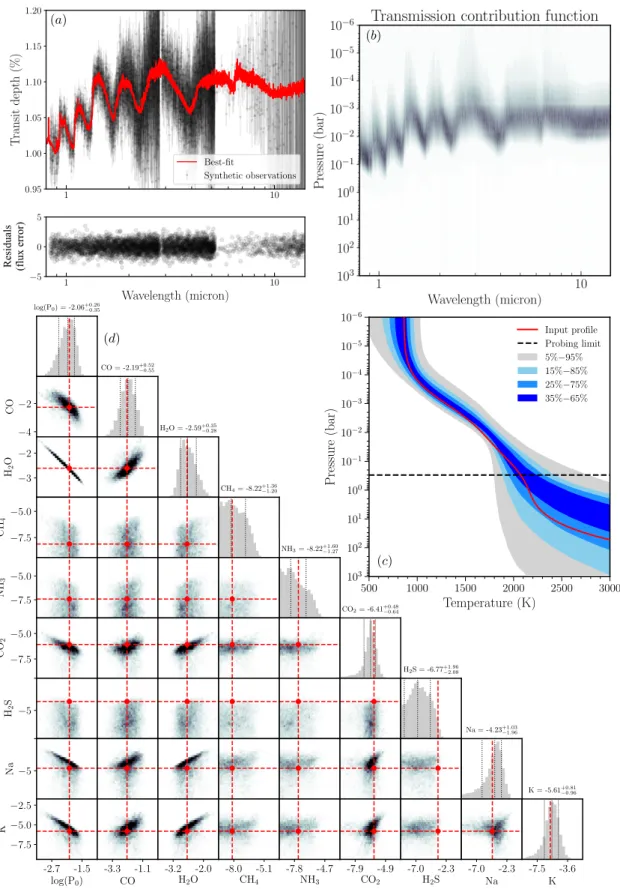
Fig. 5.Retrieval using mockJWSTemission spectra of a TrES-4b-like planet. Panel (a), top: synthetic observations (black circles)
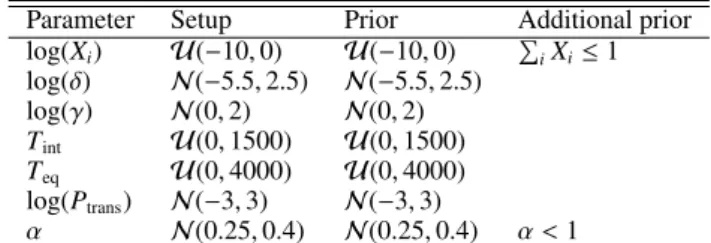
Parameter Setup Prior Additional prior
log(Xi) U(−10,0) U(−10,0) PiXi≤1
log(δ) N(−5.5,2.5) N(−5.5,2.5)
log(γ) N(0,2) N(0,2)
Tint U(0,1500) U(0,1500)
Teq U(0,4000) U(0,4000)
log(Ptrans) N(−3,3) N(−3,3)
α N(0.25,0.4) N(0.25,0.4) α <1
Table 6.Distributions used to sample the walker positions and
prior choice.U stands for a uniform distribution, with the two parameters being the range boundaries.N stands for a normal distribution, with the two parameters being the mean value and standard deviation. The unit ofδis bar−1, the unit ofTintandTeq
is K, and the unit ofPtransis bar.
setup. The parameter values of the temperature profile priors were guided by fitting our temperature model (Equation15) to the temperature structures published inMolli`ere et al. (2017).
Molli`ere et al.(2017) contains a selection of self-consistent
mod-els (clear and cloudy) for transiting planets.
We note that we allow maximum values of 4000 K for theTeq
parameter of the temperature model (Equation15), even though the line opacity database only goes up to 3000 K, after which the respective opacities are taken to be constant at their 3000 K value. However, in the retrieval example of the hot Jupiter pre-sented in this study (TrES-4b, withTeq ∼1800 K), the deepest atmospheric layers, which are hotter than 3000 K, are not probed by outgoing radiation or the grazing stellar rays (see contribu-tion plots and probing limits in Panels b and c in Figures5and
6below). In addition, keeping the parameters of the temperature model flexible (e.g.Teq up to 4000 K) is useful for letting the
retrieval find the P-T parameters that best describe the data. If the αparameter (see Equation15) is very large (but less than one), for example, it can strongly decrease the atmospheric tem-perature, even at highTeqvalues. Lastly, while the line opacities are constant forT >3000 K, the radiative source function, and the atmospheric scale height, are not. So if the Teq > 3000 K choice may lead to situations where regions hotter than 3000 K are sampled by the outgoing flux, this flux will still be high, and the transit radius large. Thus, the retrieval may ‘tell’ the user that it retrieves temperatures in excess of 3000 K, from which point on one would have to be extremely careful in one’s interpretation of the retrieval results.
100,000 samples were drawn for the pre-burn run, then a chain was started to draw 1,000,000 samples, with the walker positions initialized in a Gauss ball around the best-fit positions of the pre-burn. As a second test we reran the retrieval starting around the median position of the first chain, and drew 1,000,000 samples, with the same outcome.
Figure 5 summarizes the results from retrieving the prop-erties of the TrES-4b-like planet with a mock JWST emission spectrum. Panel (a) shows the input synthetic observations and the best-fit spectrum. The fit is excellent, this is further corrob-orated by the residual plot of Panel (a), which shows that the residuals scatter about zero, with most values within 2σ.
Panel (b) of Figure 5 shows the emission contribution function of the best-fit spectrum, which was calculated using Equation4. One can see that pressures larger than 4 bar cannot be probed. The temperature distribution at lower altitudes arises from the analytic shape of the temperature profile.
Panel (c) shows the distribution of retrieved temperature pro-files and the input profile. It also displays the probing limit
(4 bar), as derived from Panel (b). Between 10−3 and 4 bar, the
P-T envelopes closely follow the position and slope of the in-put profile. This is also where most of the spectrum contributes, see Panel (b). At lower pressure the retrieval fails to derive the temperatures correctly; here the emission contribution function is very small. At larger pressures the temperature appears to be well constrained. Because this high pressure region cannot be probed, its retrieved temperature is fully determined by the pre-dictions of the temperature model.
Panel (d) displays the 2-d and 1-d projections of the pos-terior distribution. The abundances of the major absorbers CO and H2O are retrieved within the 16-84 % percentile boundaries
of the 1-d posteriors. If the 1-d posteriors were identical to a Gaussian distribution these percentile boundaries would corre-spond to the 1-σerror bars.
For all the other species, that is for CH4, NH3, CO2, H2S, Na
and K, only upper limits can be retrieved. The peak value of the CO2mass fraction is almost identical to the input value, but there
exists a signifiant probability tail towards lower abundances. For Na and K quite large upper limits are retrieved for the mass frac-tions, which is possible especially as they can only affect the spectrum at the blue end of the spectrum at 0.8 micron, where only little flux escapes the planet. Moreover, the strong doublet lines of Na and K do not fall within the wavelength range of the synthetic JWST observations, and hence they can only affect the spectrum by virtue of their line wings.
5.2.2. Transmission spectra
In this section we describe the results from retrieving the prop-erties of the TrES-4b-like planet with a mock JWST transmis-sion spectrum. We again used 240 walkers, a pre-burn run with 100,000 samples, and then drew 1,000,000 samples, initializing the walkers around the best-fit position of the pre-burn. Figure6
summarizes the results of the retrieval.
In Panel (a) the input synthetic observations are shown and the best-fit spectrum of the retrieval. The fit appears to be excel-lent, just as in the case of the emission spectrum retrieval. The residuals scatter about zero again (see lower panel of Panel a), with most values within 2σ.
Panel (b) of Figure 6 shows the transmission contribution function for the best-fit spectrum, calculated using Equation8. One sees that pressures larger than 0.3 bar cannot be probed, and that all temperature information at lower altitudes arises from the analytic shape of the temperature profile, and the parame-ter distribution of the temperature profile, which is sensitive to pressures smaller than 0.3 bar.
Panel (c) shows the distribution of retrieved temperature pro-files, the input profile, as well as the probing limit (0.3 bar), which is derived from Panel (b). TheP-T envelopes closely fol-low the position and slope of the input profile. The largest devi-ation is atP∼0.01 bar, where the input temperature profile only falls within the 15 to 85 % envelope (i.e. still within the ‘1-σ range’).
Finally, the 2 and 1-d projection of the full posterior is shown in Panel (d) of Figure 6, for all other parameters of interest; namely the reference pressureP0, which is retrieved very well, and the log-mass fractions of all atmospheric absorbers.
For the absorbers with high abundance in the input model, i.e. CO and H2O, the abundances are correctly retrieved, that
is the input value falls within the 15 to 85 % percentile val-ues (“1-σ range”) of the retrieved values. This also holds for CO2, Na, and K, although they are of much lower abundance.