COMPUTATIONAL TOOLS TO AID THE DESIGN AND DEVELOPMENT OF A GENETIC REFERENCE POPULATION
Catherine E. Welsh
A dissertation submitted to the faculty of the University of North Carolina at Chapel Hill in partial fulfillment of the requirements for the degree of Doctor of Philosophy in the Department
of Computer Science.
Chapel Hill 2014
Approved by:
Leonard McMillan
Wei Wang
Jan Prins
ABSTRACT
CATHERINE E. WELSH. COMPUTATIONAL TOOLS TO AID THE DESIGN AND DEVELOPMENT OF A GENETIC REFERENCE POPULATION.
(Under the direction of Leonard McMillan.)
Model organisms are important tools used in biological and medical research. A key com-ponent of a genetics model organism is a known and reproducible genome. In the early 1900s, geneticists developed methods for fixing genomes by inbreeding. First generation genetic models used inbreeding to create disease models from animals with spontaneous or stimulated mutations. Recently, geneticists have begun to develop a second generation of models which better represent the human population in terms of diversity. One such model is the Collaborative Cross (CC), which is a mouse model derived from 8 founders. I have been involved in developing the CC since its early stages. In particular, I am interested in speeding up the inbreeding process, since it currently takes an average of thirty-six generations to achieve complete fixation.
In loving memory of my mother,
ACKNOWLEDGEMENTS
I would like to thank my advisor, Leonard McMillan, for his patience, his encouragement to pursue these ideas, for continually asking me to do a little more or a little better, and for his new perspectives that often seemed wrong to me at first but never were.
To my other committee members, thank you for your wonderful insights and ideas that have enriched this research and encouraged me to pursue angles and projects that I would not have otherwise. They are Wei Wang, Fernando Pardo-Manuel de Villena, Jan Prins and William Valdar.
I am also grateful for my truly supportive lab members throughout this experience. Thank you to Ping Fu, Jeremy Wang, James Holt, Katy Kao, and many others throughout the years with whom I interacted.
For my Bandidos crew over the years, Tabitha Peck, Laura Kassler, David Millman, Darrell Bethea, Alana Libonati, Robby Cochran, and the occasional guest appearances by Brittany Fasy, I am very thankful. These Friday lunchtime sessions kept me sane throughout graduate school and were often the highlights of my week!
TABLE OF CONTENTS
LIST OF FIGURES . . . xi
LIST OF TABLES . . . xvi
1 INTRODUCTION . . . 1
1.1 Selective Breeding . . . 2
1.2 Isogenics . . . 2
1.3 Combining Inbreeding and Selection . . . 3
1.4 Thesis Statement . . . 4
1.5 Organization . . . 5
2 BACKGROUND . . . 6
2.1 Genomic Data . . . 6
2.1.1 SNPs . . . 7
2.1.2 Microarrays . . . 7
2.1.3 High-throughput sequencing . . . 8
2.2 Recombination and Breeding . . . 9
2.2.1 Genetic Reference Populations . . . 10
2.2.2 Collaborative Cross . . . 11
2.2.3 Diversity Outbred . . . 12
3 MARKER-ASSISTED INBREEDING THEORETICAL ANALYSIS . . . 16
3.1 Approach . . . 17
3.2 Experiments and Results . . . 24
3.2.1 Nonmarker-assisted breeding schemes . . . 25
3.2.2 Marker-assisted inbreeding . . . 28
3.2.3 Selected advanced intercrosses . . . 31
3.2.4 Low-resolution sampling . . . 32
3.3 Conclusion . . . 34
4 DESIGNING MICRO-ARRAYS FOR MAXIMUM INFORMATIVENESS . . . 36
4.1 MUGA . . . 37
4.1.1 Database of Available Probes . . . 38
4.1.2 Design . . . 39
4.1.3 Samples Run on MUGA . . . 41
4.1.4 Performance on MUGA . . . 41
4.2 MegaMUGA . . . 48
4.2.1 Design . . . 48
4.2.2 Samples Run on MegaMUGA . . . 54
4.2.3 Performance on MegaMUGA . . . 54
4.3 Conclusion . . . 54
5 MAI IN PRACTICE . . . 57
5.1 Analysis Tools . . . 57
5.1.1 Haplotype Reconstructions . . . 57
5.1.2 Line Quality Control . . . 59
5.1.3 Breeder Selection . . . 65
5.2 Conclusion . . . 70
6 HIGH-THROUGHPUT SEQUENCING DATA . . . 75
6.1 Sequence Data . . . 76
6.2 HMM Algorithm . . . 77
6.2.1 Variants . . . 77
6.2.2 Emission Probabilities . . . 77
6.2.3 Transition Probabilities . . . 80
6.2.4 Viterbi Solution . . . 81
6.3 Founder-pair Resolution . . . 83
6.4 Breakpoint Mapping of HTS data . . . 84
6.4.1 Comparison with Refined Breakpoint Solution . . . 84
6.4.2 Comparison to Genotype Solutions . . . 88
6.4.3 Read Coverage Analysis . . . 95
6.5 Conclusion . . . 101
7 CONCLUSION AND FUTURE WORK . . . 102
7.1 Theoretical Marker-Assisted Techniques . . . 102
7.1.1 Future Work . . . 103
7.2 Tools for Analysis of Live Mice . . . 103
7.2.1 Future Work . . . 104
7.3 High-Throughput Sequencing Data . . . 104
7.3.1 Future Work . . . 105
APPENDIX A SEQUENCE SIMILARITY MAPS . . . 107
LIST OF FIGURES
2.1 Depiction of a SNP. . . 7 2.2 Collaborative Cross breeding scheme. . . 12 2.3 Diversity Outbred breeding explanation. . . 14 3.1 The average number of founder segments in eight-way RILs
at various generations of inbreeding. . . 17 3.2 The number of generations to complete fixation (A) and the
number of resulting founder segments (B) in two-way and
eight-way RILs. . . 18 3.3 This image shows all possible JH states between a potential
mating-pair and illustrates my notion of a genomic segment. . . 19 3.4 A state diagram showing the transitions between all JH states
in a single generation. . . 21 3.5 A histogram of segments colored according to their JH state
as a function of generation. . . 22 3.6 This figure shows the pedigree diagrams for the alternating
backcrosses: father-daughter backcross with the mother-son backcross (A) and the father-daughter with the random
sib-mating (B). . . 26 3.7 A comparison of five breeder selection alternatives for
gener-ating an eight-way RIL, showing the number of generations to reach complete fixation (A) and the total number of segments
(B) found in the final inbred lines. . . 27 3.8 Compares the number of generations it takes to achieve
com-plete fixation for 5 breeding schemes that make different
as-sumptions about the available pool of breeders. . . 30 3.9 CHF as a function of number of generations. . . 31 3.10 Histogram of size of segments missed when conducting low
4.2 Distribution of the original 9,000 SNPs on MUGA in terms of
location on chromosomes. . . 42
4.3 Distribution of the final 7,541 MUGA SNPs in terms of lo-cation on chromosomes (left plot) and spacing between SNPs (right plot). . . 43
4.4 Intensity plots of four markers, colored by genotype calls from Illumina. . . 47
4.5 Recombination events on a chromosome basis. . . 51
4.6 Distribution of the final 77,808 MegaMUGA SNPs in terms of location on chromosomes. . . 52
4.7 Break down of the final distribution of SNPs by type for which they were originally chosen. . . 53
5.1 Haplotype reconstruction of a CC mouse sample. . . 60
5.2 Quality Control Report screenshot. . . 61
5.3 Distribution of shared recombination events before and after identifying related samples. . . 63
5.4 Comparison table created by Choose Breeders tool. . . 66
5.5 Combined haplotype reconstruction images of proposed breed-ers as created by the Choose Breedbreed-ers tool. . . 67
5.6 Simulate Matings tool output. . . 69
5.7 Partial view of the pedigree of the OR3252 CC line as well as the genome of obligate ancestors and the genome of the line based on MUGA genotypes. . . 71
5.8 Residual heterozygosity in distributable lines. . . 72
5.9 The UNC Systems Genetics Core web site. . . 73
6.1 HMM emission probabilities diagram for one bin. . . 79
6.2 HMM transition probabilities. . . 81
6.4 Sequence similarity maps for three founder-pairs and histogram
of spacing between informative SNPs for all founder-pairs. . . 85
6.5 Histogram of distance between HMM solution and refined re-combination breakpoint. . . 87
6.6 Depiction of all informative SNPs between A/J and NOD/ShiLtJ on Chromosome 13 from 101.5Mb to 104.0Mb. . . 88
6.7 Histogram of distance between informative SNPS in the re-fined breakpoint solution. . . 89
6.8 Comparison of HTS full coverage solutions with MUGA and MegaMUGA solutions for OR867m532. . . 92
6.9 Comparison of HTS full coverage solutions with MUGA and MegaMUGA solutions for OR1237m224. . . 93
6.10 Comparison of HTS full coverage solutions with MUGA and MegaMUGA solutions for OR3067m352. . . 94
6.11 Comparison of HTS full coverage solution for OR867m352 with 4x and 0.25x coverage solutions. . . 98
6.12 Comparison of HTS full coverage solutions for OR1237m224 with 4x and 0.25x coverage solutions. . . 98
6.13 Comparison of HTS full coverage solutions for OR3067m352 with 4x and 0.25x coverage solutions. . . 99
6.14 Histograms of the delta between the maximum position and minimum position found at each recombination among the 10 runs at each coverage level. . . 100
A.1 Sequence similarity map for CC founders A (A/J) and B (C57BL/6J). . . 108
A.2 Sequence similarity map for CC founders A (A/J) and C(129S1/SvImJ). . . 108
A.3 Sequence similarity map for CC founders A (A/J) and D (NOD/ShiLtJ). . . 109
A.4 Sequence similarity map for CC founders A (A/J) and E (NZO/HlLtJ). . . 109
A.5 Sequence similarity map for CC founders A (A/J) and F (CAST/EiJ). . . 110
A.7 Sequence similarity map for CC founders A (A/J) and H (WSB/EiJ). . . 111 A.8 Sequence similarity map for CC founders B (C57BL/6J) and C (129S1/SvImJ). 111 A.9 Sequence similarity map for CC founders B (C57BL/6J) and
D (NOD/ShiLtJ). . . 112 A.10 Sequence similarity map for CC founders B (C57BL/6J) and E (NZO/HlLtJ). . 112 A.11 Sequence similarity map for CC founders B (C57BL/6J) and F (CAST/EiJ). . . 113 A.12 Sequence similarity map for CC founders B (C57BL/6J) and
G (PWK/PhJ). . . 114 A.13 Sequence similarity map for CC founders B (C57BL/6J) and
H (WSB/EiJ). . . 114 A.14 Sequence similarity map for CC founders C (129S1/SvImJ)
and D (NOD/ShiLtJ). . . 115 A.15 Sequence similarity map for CC founders C (129S1/SvImJ)
and E (NZO/HlLtJ). . . 115 A.16 Sequence similarity map for CC founders C (129S1/SvImJ)
and F (CAST/EiJ). . . 116 A.17 Sequence similarity map for CC founders C (129S1/SvImJ)
and G (PWK/PhJ). . . 116 A.18 Sequence similarity map for CC founders C (129S1/SvImJ)
and H (WSB/EiJ). . . 117 A.19 Sequence similarity map for CC founders D (NOD/ShiLtJ)
and E (NZO/HlLtJ). . . 117 A.20 Sequence similarity map for CC founders D (NOD/ShiLtJ)
and F (CAST/EiJ). . . 118 A.21 Sequence similarity map for CC founders D (NOD/ShiLtJ)
and G (PWK/PhJ). . . 118 A.22 Sequence similarity map for CC founders D (NOD/ShiLtJ)
and H (WSB/EiJ). . . 119 A.23 Sequence similarity map for CC founders E (NZO/HlLtJ) and
A.24 Sequence similarity map for CC founders E (NZO/HlLtJ) and
G (PWK/PhJ). . . 120 A.25 Sequence similarity map for CC founders E (NZO/HlLtJ) and
LIST OF TABLES
2.1 Letter and color codes for CC Founders. . . 13
4.1 Comparison of biological replicate samples run on MUGA. . . 44
4.2 Entropy scores for micro-array comparison. . . 45
4.3 Comparison of biological replicate samples run on MegaMUGA. . . 55
5.1 Genome-wide CC founder contribution. . . 65
6.1 Comparison of HTS to genotype solutions. . . 90
CHAPTER1: INTRODUCTION
The rediscovery of Gregor Mendel’s Laws of Inheritance in 1900 launched a new wave of genetic studies. In particular, scientists wished to verify Mendel’s laws in organisms other than plants since it was unknown if the laws would hold true for animals[40]. The mouse was chosen for these particular studies as it is ideally suited for genetic analysis since it has a relatively short generation time (about 10 weeks from birth to giving birth), it breeds easily in captivity and mice are easily housed in small cages[53]. An additional benefit is that due to mouse fanciers in the 1800s, numerous variants of mice had been derived which had visible phenotypes. A system-atic analysis of inheritance and genetic variation in mice as well as other mammals ensued[53]. These early studies utilized selective breeding to verify recessive and dominant trait inheritance patterns. They also brought to light the existence of more than two alleles at a locus, recessive lethal alleles, and interactions among unlinked genes[53].
1.1 Selective Breeding
Quantitative genetics deals with the inheritance of complex traits that are controlled by many loci, each with relatively small effects, and by environmental influences such as diet and exercise[22]. In order to study quantitative genetics, selective breeding, which refers to the sys-tematic breeding of animals in order to choose certain qualities in them, is often used. Breeders will select for quantitative phenotypes such as body weight, growth rate, feed efficiency, feed intake, body composition and litter size. By selecting for these traits, scientists can then see how far artificial selection can change a trait and how many generations are needed to reach a limit, if a limit can be reached[53]. During the selection process targeted traits are chosen intention-ally, however, without specific controls, other traits may also be selected inadvertently, such as fertility and docility.
As technology advanced, it was possible to select for particular genotypes or genes. Through selection for quantitative traits, a number of mutations and variants were formed. In the analysis of these mutants, it is often not possible to distinguish between subtle effects due to the mutation itself and effects due to other genes within the background of the mutant strain. To make this distinction, it is essential to be able to compare animals in which differences in the genetic background have been eliminated as a variable in the experiment. This is accomplished through the placement of the mutation into a genome of another mouse strain. To do this, genotyping of the area surrounding the gene is done at each level of breeding and offspring with the gene of interest are selected for further breeding[53].
1.2 Isogenics
to as selfing. However, in laboratory animals, inbred strains are either achieved through a series of backcrossing, mating offspring back to their parent (or genetic equivalent), or through sibling matings. In mice, to create a new inbred strain from two outbred strains, repeated brother-sister matings are made for several generations to achieve fixation. A classic rule-of-thumb is that at least 20 generations are necessary to reach homozygosity for nearly all genetic loci[22]. These inbred strains are said to be isogenic because all individuals are genetically identical.
Since isogenic animals have fixed genomes, they are easily reproducible. Mating together two isogenic animals will always produce another isogenic animal, which enables reproducible studies and the integration of data over both time and space. The only way an inbred strain can change genetically is as a result of new mutations, which are relatively rare. Another advantage of inbred strains is that many can serve as disease models due to their lack of buffering alleles, which makes them susceptible to cancer, diabetes, obesity and other diseases. Therefore, inbred strains can be studied as models of these conditions.
1.3 Combining Inbreeding and Selection
the donor strain DNA in the specified regions. This genotyping was done on a small scale, usually with a few loci chosen at points of interest.
Through advances in technology, it now costs about the same amount to get full-genome genotypes as the small scale genotyping used to cost. Full-genome genotyping allows us to have better control over the final inbred strains. In congenics, this means less donor strain in the genomic regions outside the chromosomal fragment of interest. By utilizing full-genome geno-types, marker-assisted or speed congenics were created, which only require about 5 generations of backcrossing. This is achieved by selecting offspring at each generation that not only retain the desired chromosomal fragment, but that also have a minimal amount of background genetic information from the donor strain in the other genomic regions. In the creation of new inbred strains, genotyping allows us to more closely track the amount of residual heterozygosity (loci that are still segregating).
1.4 Thesis Statement
Through monitoring of genome-wide genotypes over multiple generations, one can engineer
user-specified genomic structures. This can be made more efficient, in terms of the number of
generations, with accurate computational models. These computational models will lead to new
breeding techniques, better breeder selection, and techniques for monitoring genomic structure.
breeder selection in the end-goal of creating a panel of inbred strains. To utilize these computa-tional models on a live mouse population, techniques for monitoring the genomic structure of the population were developed, as described in Chapters 4 and 5 of this thesis. Chapter 6 discusses the process of validating the results from Chapters 4 and 5.
1.5 Organization
The rest of this thesis is organized as follows:
• Chapter 2presents biological background such as the basics of genetics and a description of the breeding population used throughout the studies in this thesis.
• Chapter 3 presents a computational simulation model used to study various breeding schemes and examine techniques for speeding up the process of inbreeding through the use of marker-assisted techniques.
• Chapter 4presents the design and development of low-cost, low-density genotyping ar-rays for monitoring the genomes of a breeding population and includes analysis of the performance of these arrays.
• Chapter 5presents the application of our theoretical results from Chapters 3-4.
• Chapter 6presents a method for determining the underlying genomic structure of a breed-ing population usbreed-ing high-throughput sequencbreed-ing data and compares those results to sim-ilar results obtained through the use of the genotyping platforms discussed in Chapter 4 and the results discusssed in Chapter 5.
CHAPTER2: BACKGROUND
2.1 Genomic Data
A gene is a molecular unit of heredity of a living organism. Genes hold the information to build and maintain an organism and pass its traits to its offspring. All organisms have genes cor-responding to various biological traits, some of which are instantly visible, such as eye color and coat colors, and some of which are not, such as blood type, increased risk for specific diseases, or the thousands of basic biochemical processes that comprise life.
An organism’s genome is comprised of the complete set of all its genes as well as the intergenic regions. Generally members of a species have a common set of genes and every cell within the organism carries the same genome. Each gene is a segment of deoxyribonucleic acid (DNA) and the genes are joined together to make up a set of very long DNA molecules called chromosomes. In diploid organisms like humans and mouse, there are two copies of each chromosome. One copy is inherited from each parent.
DNA is comprised of a sequence of nucleotides and the four primary DNA bases found in nucleotides are Adenine(A), Cytosine(C), Guanine(G), and Thymine(T). Each base binds with another specific base (T with A and C with G). A DNA molecule is comprised of a primary sequence and a “complementary” copy that allows it to self replicate, as each acts like a template for the other sequence.
Figure 2.1: Depiction of a SNP. This image shows a subset of DNA from three different organ-isms. While the majority of base pairs for these three organisms are identical, at the denoted SNP there are three possible combinations of G/A alleles.
2.1.1 SNPs
A SNP is a DNA sequence variation occurring when a single nucleotide differs between two sequences, resulting from a substitution of one nucleotide for another. For example, two sequenced DNA fragments from different individuals, AAGCCTA and AAGCTTA, contain a difference in a single nucleotide. In this case we say that there are two alleles. Almost all common SNPs have only two alleles or are biallelic. Figure 2.1 is depicting a SNP, and shows a subset of the DNA from three different organisms. While the majority of base pairs for these three organisms are identical, at the denoted SNP there are three possible combinations of G/A alleles. To determine the allele at a SNP location for a particular sample, genotyping needs to be done. In genome-wide studies, often a DNA microarray is used for this purpose.
2.1.2 Microarrays
to build two genome-wide SNP arrays. In a popular model organism like the mouse, designing an array consists of selecting a subset of known and reliable SNPs at specified genomic locations that segregate between strains of interest.
A number of companies including Affymetrix and Illumina offer the ability to design custom arrays. While both companies use slightly different technologies, the basic idea is the same. The customer selects known SNPs and reports the surrounding DNA sequence for that SNP. Since a complementary strand of DNA will be created for each of the chosen SNP locations, it is important that the area surrounding the SNP has a unique DNA sequence. A complementary strand of DNA is then designed for each of the SNPs and placed on the microarray. A sample’s DNA is then washed over the plate and the complementary DNA strands will hybridize or “stick” to the sample DNA in the correct locations. Fluorescently labeled target sequences that bind to a probe sequence generate a signal and the total strength of the signal depends upon the amount of target sample binding to the probes present on that spot. Microarrays use relative quantitation in which the intensity of a feature is compared to the intensity of the same feature under a different condition, and the identity of the feature is known by its position. This intensity ratio is then normalized and used to determine the genotype (A, T, C, or G) for a particular SNP location.
2.1.3 High-throughput sequencing
Before a sample is sequenced, its DNA is replicated and cleaved into small pieces (about 50-1000 base pairs). Each of these DNA pieces is then run through the sequencer and the nucleotides are determined. Once the nucleotide sequences are determined, it is necessary to assemble the short reads in their correct order to determine the whole genome DNA sequence. This can be done using de novo alignment (meaning the DNA sequence is not previously known) or the reads can be aligned to a known reference genome. The coverage level of the HTS data is determined by the number of times the DNA was replicated before being sequenced. The coverage refers to the average number of reads that should pileup at each genomic position. Areas of the genome that are highly repetitive often have very high pileups. Since HTS samples the genome randomly, occasionally no reads will align to particular areas of the genome making it difficult to resolve the genotypes for certain regions. However, once HTS data has been properly aligned, it can be used to ascertain genotypes, determine recombination event locations, and accurately infer ancestry as I show in Chapter 6.
2.2 Recombination and Breeding
can also occur during mitosis, this process does not create new allele combinations except by mutation. Moreover, recombinations during mitosis do not impact future generations (i.e. the germ line).
The main impact of meiosis is the creation of genetic diversity by allowing offspring to inherit different allele combinations from their parents. Organized breeding schemes are utilized in biological experiments to create desired allele combinations in offspring. Often the desired result are isogenics or inbred strains, which can be replicated indefinitely as both parents will have identical copies of all chromosomes (except for X and Y). When a panel of such animals are derived from the same founder strains, this is referred to as a genetic reference population.
2.2.1 Genetic Reference Populations
Genetic reference populations (GRPs) are defined as sets of individuals with fixed and known genomes that can be replicated indefinitely. Typically they consist of dozens to hundreds of inbred lines derived from a set of common ancestors (founders). GRPs have been developed for many organisms, including yeast, plants, flies, and mammals [4, 18, 11, 3, 31, 19]. GRPs are popular for the study of complex traits and biological systems in both medical and life sci-ence applications because genotyping is required only once (described as the “genotype once, phenotype many times” paradigm); replicate individuals can be produced with the same geno-type allowing for optimal case/control and gene-by-environment designs, and custom analysis tools[59, 13, 29]. GRPs are also attractive because the phenotypic, genetic, and genomic data associated with each line can be integrated across labs, experiments, and time.
Project [41] and combinations of diversity panels and pairwise panels [6]. Key parameters that determine the usefulness of GRPs for the analysis of complex traits are the number of lines; the density, distribution, and functional significance of the genetic variation present in the GRP; the number and distribution of unique recombination sites; the presence of population structure; and the level of inbreeding and genetic drift.
2.2.2 Collaborative Cross
An example of a mouse GRP is the Collaborative Cross (CC)[17]. The CC is a multi-parental recombinant inbred panel derived from a set of eight genetically diverse inbred labora-tory mouse strains. The set of founders consists of five classical inbred strains (A/J, C57BL/6J, 129S1/SvImJ, NOD/ShiLtJ, NZO/HlLtJ) and three wild-derived inbred strains which were se-lected to represent three Mus musculus subspecies(CAST/EiJ, PWK/PhJ, WSB/EiJ). They were chosen to capture a high level of genetic diversity, representing on average 90% of known genetic variation in laboratory stocks across all 1-Mb intervals[49].
The CC lines were generated via a funnel breeding scheme that combined the eight founder genomes in three intercross generations prior to repeated generations of inbreeding through sib-ling mating (Figure 2.2).The eight founder strains capture a much greater level of genetic di-versity than existing RIL panels or other extant mouse GRPs, and the genetic variants are more uniformly distributed across the genome than in other GRPs [49, 30, 63, 65]. As seen in Figure 2.2, the eight CC founders have been assigned letters A-H as well as a color. These letter and color codes are used consistently throughout all publications about the CC, including this thesis, and are shown in Table 2.1.
Figure 2.2: Collaborative Cross breeding scheme. Each independent CC strain begins with a funnel breeding stage that mixes eight founders, which are crossed for two generations, G1 and G2. The lines are then inbred for at least 20 generations to obtain recombinant inbred lines. CC lines are regularly genotyped after their 6th generation of inbreeding to monitor their residual heterozygosity, detect breeding errors, and to accelerate the inbreeding of selected lines.
CC lines[17]. Of those 350, about 70 of these lines are currently considered completed and are available for distribution. As reported[17], there is little long-range linkage disequilibrium in the CC population and the recombinations are independent.
2.2.3 Diversity Outbred
CC Founder Letter Color
A/J A Yellow
C57BL/6J B Black
129S1/SvImJ C Pink NOD/ShiLtJ D Dark Blue
NZO/HlLtJ E Light Blue CAST/EiJ F Green
PWK/PhJ G Red
WSB/EiJ H Purple
Table 2.1: Letter and color codes for CC Founders.
occurred in the early generations of CC breeding to effectively jump-start recombination density in the DO population.
Since the DO and CC populations are derived from a common set of eight founder strains, they both capture, in theory, the same set of alleles. However, while each CC inbred strain represents a fixed and reproducible genotype, each DO animal is a unique individual with one of an effectively limitless combination of the segregating alleles. This makes the DO an ideal resource for high-resolution genetic mapping.
2.3 Related Work
Figure 2.3: Diversity Outbred (DO) breeding explanation[55].
mice, this requires, on average, a minimum of 20 generations [22] and assuming an average of four generations per year, it takes a minimum of 5 years to create a new RIL. Moreover, a large fraction of the started RILs fail, presumably as the result of genetic incompatibilities affecting survival and reproduction [53].
Many recent efforts to generate RILs have focused on multiway crosses where more than two parental lines are initially mixed before inbreeding. In 2005, Broman [8] ran simulations to determine the average number of generations required for two-way and eight-way RILs to reach 99% fixation and complete fixation. He also tracked the number of segments generated through recombination in inbred lines and used it as a comparison between the genetic diversity of two-way and eight-way sib-mating RILs.
have demonstrated a reduction in the number of generations of backcrossing from 10 genera-tions to five. This reduction was achieved by selecting the progeny with the lowest residual het-erozygous fraction to cross back to the background strain. These selection criteria have evolved overtime, as technology has allowed for more rapid and specific genotyping [23].
CHAPTER3: MARKER-ASSISTED INBREEDING THEORETICAL ANALYSIS
Broman [8] showed through simulation that eight-way RILs take on average 26.7 genera-tions of sib-mating to reach 99% fixation, and 38.9 generagenera-tions, on average, to reach complete fixation. Although a major source of genetic variation in a RIL is derived from the choice of founder strains, I focus on the additional genetic variations introduced by mixing of allele com-binations via recomcom-binations between founder genomes. This is the primary source of genetic variation between RILs. Therefore, the number of distinct founder segments, defined as the re-gions between recombination breakpoints on the RIL chromosomes, can be used as a measure of genetic diversity. From now on, I refer to these distinct founder segments simply as segments.
Recombinations in early generations increase diversity, but eventually diversity peaks and the process of inbreeding leads to a loss of segments. To verify this, I simulated 100,000 eight-way RILs and tracked the number of segments in each line at every generation until the simulated lines reached complete fixation. In an eight-way cross, the peak in diversity is reached at the seventh generation of inbreeding on average and before 10 generations of inbreeding for 75% of line starts (Figure 3.1). Therefore, I will consider 10 generations of inbreeding as past the point of peak diversity. If inbreeding acceleration is started before this peak is reached, the resulting inbred lines are likely to see a reduction in the number of segments. Therefore, unless otherwise specified, I use traditional methods for constructing RILs in the first 10 generations, after which I apply various methods for accelerating the inbreeding process.
Figure 3.1: The average number of founder segments in eight-way RILs at various generations of inbreeding. This figure is based on 100,000 simulations, and the number of segments was tracked until they reached complete fixation. The average peak in the number of segments occurs at generation 7 and before generation 10 for 75% of all lines. Therefore, I consider generation 10 to be past the point of peak diversity.
without substantially impacting the overall genetic architecture of the inbred lines.
In this chapter, I address accelerating the inbreeding process of RIL creation by using a combination of alternative breeding strategies and marker-assisted inbreeding (MAI) techniques. 3.1 Approach
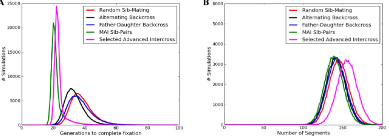
Figure 3.2: The number of generations to complete fixation (A) and the number of resulting founder segments (B) in two-way and eight-way RILs. On average, two-way RILs take 35.92 generations to reach complete fixation and have 91.95 segments. Eight-way RILs take 38.21 gen-erations and have 145.12 segments on average. These figures are based on 100,000 simulations and are consistent with previous simulations [8].
Despite the differences in the underlying representation, my simulator produces results nearly indistinguishable from those presented by Broman [8]. Figure 3.2 shows the distribution of the number of generations to complete fixation and number of segments for both the two-way and eight-way sib-mating RILs based on the simulation of 100,000 RILs. For a randomized eight-way RIL my simulations show that it takes an average of 38.21±7.1 (SD) generations of sib-matings to reach complete fixation. The genomes of the resultant inbred lines have an aver-age of 145.1±12.48 segments in their mosaic structure. Furthermore, 25.72±3.16 generations of sib-mating on average are needed to reach 99% fixation. These baseline metrics are used for comparison against my accelerated inbreeding simulations. My analysis is based on an initial funnel-breeding scheme like that used in the eight-way Collaborative Cross (CC) [16, 17], where the mixing of eight inbred lines occurs in three initial crossing stages, followed by successive generations of sib-matings until the line becomes fully inbred.
from each parent of a potential breeding pair and depicts all possible JH states. The inbred state is achieved when both male and female samples are homozygous for the same founder state. I call this state same-same (SS). Another possible state involves a breeding pair that is heterozygous with alleles from two founders while the mate is homozygous. I call this different-same (DS). This state occurs in two forms,DS2when the heterozygous gene shares a founder allele with the homozygous allele of its mate, andDS3, when the heterozygous gene shares no founder alleles with its mate. The third state is opposite-same (Ss), where the male is homozygous for one founder and the female is homozygous for another. The final state is different-different (DD), where both male and female are heterozygous. This state comes in three variations, involving, two, three, and four founders, respectively. The two-founder state, calledDD2, occurs when both male and female are heterozygous between the same founder alleles. DD3 refers to when both male and female are heterozygous but share one common founder allele. DD4 occurs when the male and female are heterozygous and do not share any founder alleles. Figure 3.4 shows a state diagram with these four states and their forms depicting all possible transitions between them in a single generation. The directed edge weights represent the probability of transitioning between JH states. A similar transition matrix, which uses thirteen states instead of my seven, has also been derived by Broman [9]. It is a simple matter to extend our JH model to two generations by finding every path of length two within the graph and inserting an edge with weight equal to the product of the two edges along its path. The weights of edges from a common source to a common destination, but passing through different intermediate states, can be added and combined into a single edge. This approach can be extended to n generations, and as n increases all of the heaviest edges eventually lead to the inbred (SS) state. For analytical expressions for extending our JH model for n generations, see [9, 17].
Figure 3.4: A state diagram showing the transitions between all JH states in a single generation. The directed edges are labeled with the transition probability. The grayed-out nodes represent transient states; once a segment moves away from these three states, there are no returning edges. Transient states tend to go away after a few generations and are rarely seen past the point of peak diversity (as shown in Figure 3.5). CC lines begin inbreeding in one of the states,DD4, DD3,, andDD2. The desired inbred state for all intervals is SS.DS2 is the most likely to become SS.
DD2is the next most likely state to become fixed. It takes at least two generations to transit from Ss to SS, as there is no direct path between these two states.
I simulated 100,000 eight-way crosses and tracked the JH states between breeder pairs at each generation, as shown in Figure 3.5. By generation 10 (after the point of peak diversity), all segments have contributions from two or fewer founders. DD4, DD3, and DS3 are transient states (see Figure 3.4), meaning that once this group of three states is left, there are no returning edges. In two-way RILs, the three transient states do not occur because there are at most two founders present. When selfing, the model further reduces to only two JH states,DD2 and SS. The transition probabilities to reach the inbred state are incorporated into my metric for selecting the best mating pair at each generation, which is discussed later in this section.
to fully inbred.
I choose the “best” breeding pair, by considering a weighted genomic mix of the JH types of all candidate mating pairs. The best pair is selected as the maximum of a weighted combination of transition probabilities for all JH segments of a given mating pair considering all chromo-somes. For each distinct JH segment of a chromosome the probability that it will become inbred in the next generation (i.e., the weight of the edge from the current JH state to the SS state) is multiplied by the chromosome fraction of the segment, and the sum is accumulated over all seg-ments on the chromosome. This calculation results in a chromosome score ranging from 0, when the entire chromosome is Ss,DD3,DD4, orDS3, to 1 when the entire chromosome is SS. This approximation ignores the relative ordering of segments, and, therefore, does not consider link-age. The individual chromosome scores are then multiplied together, modeling their independent segregation, to arrive at the total pair score. Therefore, I assign a score for a given mating pair as:
Score(n, m) =
N Y
i=1
X
J HSeqn,m∈Chri
p(J HSeqn,m →SS)
kJ HSeqn,mk kChrik
(3.1)
This score is an approximation of the actual likelihood that the entire genome will become inbred in the next generation. I refer to this score as the weighted state metric (WSM).J HSeqn,m represents a JH segment on the specified chromosome i induced by the pairing n,m, and the best pair is the maximum of this score over all possible pairs n,m. In self-pollinated species, my score simplifies to a scaled version of the FGF because the only relevant states areDD2and SS, which has been described previously [7].
3.2 Experiments and Results
marker-assisted advanced intercross, which modifies the breeding scheme to choose sib-pairs to increase segments until either a specified generation or a desired number of segments is reached; it then reverts to choosing sib-pairs to accelerate inbreeding. Through simulations, I track the average number of generations to fully inbred and to 99% inbred as well as the average number of segments present in the inbred lines to compare the different breeding schemes.
The simulator is written in Python and runs on a Dell Studio XPS with 8GB RAM, with dual-threaded quad-core processors. It takes approximately 5.5 hours to complete 100,000 sim-ulations of eight-way RILs.
For the purposes of this analysis, the eight-way CC funnel breeding scheme was used, but my simulator also supports the input of any breeding scheme using pedigree files. It has also been used to simulate two-way RILs, F2 crosses, and outbred populations.
To test my MAI methods, I used the developing CC [17] and a low-density genotyping plat-form I codesigned, referred to as the Mouse Universal Genotyping Array (MUGA)(see Chapter 4). The SNPs on MUGA are uniformly distributed with an average spacing of 325 Kb and a standard deviation of 191 Kb. In an eight-way cross, the genotypes at multiple markers (at a minimum three) are needed to distinguish among the founders. The founder assignments and re-combination breakpoints are inferred from the genotypes using a hidden Markov model similar to the ones described by Mott et al. [38], Zhang et al. [47], and Liu et al. [36]. Because multiple markers are needed to distinguish each founder, the effective founder-ascertainment resolution of MUGA is approximately 1 Mb.
3.2.1 Nonmarker-assisted breeding schemes
analysis of Broman [8], which identified a substantial advantage for selfing when compared to sib-mating. Selfing in two-way plant RILs takes on average 10.5 generations to reach complete fixation, which is a substantial reduction from the 35 generations needed for two-way sib-mating. Since offspring are exactly 50% related to their parents, but only on average 50% related to their siblings, when selecting breeders at random, a backcross guarantees a level of similarity that sib-matings cannnot. A second motivation for using backcrosses is that loss of fertility in the creation of RILs is a major issue. Valuable time can be lost when unproductive sib-matings are set up. Therefore, backcrossing allows the use of known-fertile samples and has been a useful fallback for preserving lines.
The first breeding scheme examined was alternating backcrosses in successive generations, father-daughter in one generation followed by mother-son in the next (Figure 3.6A). This scheme has many practical advantages in that it leverages known-fertile samples. Furthermore, this strat-egy also serves as a useful fallback for preserving lines. I simulated this approach starting after the point of peak diversity, with a backcross between a father and daughter followed by a back-cross between a mother and son in the next generation (each breeder is used in two successive generations, alternating dam and sire). This process was repeated for each subsequent generation until complete fixation was achieved. Alternating backcrosses achieves a reduction in the num-ber of generations to complete fixation with an average numnum-ber of generations of 33.45±5.88 (Figure 3.7). This represents a reduction of nearly five generations over randomized mating and a substantial reduction in variance. It decreases the number of segments in the resulting inbred lines to 141.21, a loss of about four segments on average. The alternating backcross also reduces the number of generations to 99% fixation to 23.45±3.11, a reduction of two generations.
backcross is followed in the next generation by a random sib-mating. This breeding scheme (Figure 3.6B) is repeated for each subsequent generation until complete fixation is achieved. The father-daughter backcross takes 37.06±7.55 generations to reach complete fixation, and the in-bred lines contain on average 142.39±12.24 segments (Figure 3.7). This breeding scheme also takes 24.70±3.54 generations to 99% fixation. Although the benefits of father-daughter mating are modest relative to random sib-mating, in practice they are compensated for by a reduction in generation time resulting from a mature and known fertile sire.
3.2.2 Marker-assisted inbreeding
The steadily decreasing cost of full-genome genotyping combined with the advantages of considering each sample’s individual full genetic makeup motivated the decision to also explore MAI techniques. The ability to compare potential breeding pairs based on full-genome genotypes allows one to choose breeding pairs with the greatest likelihood of producing inbred offspring. The Ss (opposite same) is the least-preferred state in a breeding pair because it has no chance of becoming inbred in the next generation, as shown in Figure 3.4. In contrast, of the noninbred states, DS2 has the greatest probability of becoming fixed in the next generation, and DD2 is the next most likely. For all MAI techniques, random sib-matings were simulated until the point of peak diversity was passed. This was followed by subsequent generations of selecting the best breeding pair, until the line reached complete fixation.
(offspring from different mating pairs of the same generation) were the next most likely, being selected 6.9%. The remaining 7.1% included mating combinations such as aunt-nephew, uncle-niece, or grandparent-grandchild. I concluded that non-sib, non-backcross matings should be used sparingly, except in the case of preserving a line.
Because sib-pairs were most often the best option, I limited subsequent simulations to se-lecting the best pair and report those statistics in Figure 3.7 and Table 1. For the MAI sib-pairs breeding scheme, random sib-matings were simulated until the point of peak diversity was reached. After this point, four female and four male offspring were simulated (4-4), all pairs were considered, and the best pair was chosen as the breeders. This process was continued until the line reached complete fixation. My model is based on generation number and may require multiple litters to achieve the four females and four males assumed in simulation.
A potential shortcoming of my model is that I report the time to inbred as a function of gen-erations, not the number of litters or calendar time required to produce enough viable offspring. However, I did perform additional simulations assuming smaller litter sizes (two females, two males), and unbalanced sex-ratio (eight total offspring with one to seven females), and compared all three sets of assumptions (4-4, 2-2, 8) to the greedy approach of setting up breeders as soon as any sibling mating pairs are available(Figure 3.8). Each of these forms of MAI was able to con-siderably reduce the number of generations to achieve inbred status regardless of sex balance or litter size. Moreover, waiting for a sufficiently large breeder-candidate set always outperformed the greedy approach of setting up matings as soon as any pair was available. These tests were done by simulating each of the above breeding schemes 100,000 times and plotting the results in terms of number of generations to complete fixation as well as the number of intervals in the final inbred lines.
Figure 3.9: CHF as a function of number of generations. This plot shows that MAI reduces the CHF among breeding pairs much faster than random sib-matings. We can see the effect as soon as the breeding scheme is modified (at the point of peak diversity).
3.9 shows that MAI reduces the CHF among mating pairs much faster than random sib-matings. As soon as the breeding scheme is altered at the point of peak diversity, the effect is apparent.
3.2.3 Selected advanced intercrosses
techniques as discussed previously are used to select the breeding-pairs until the line is fixed. I found that it took on average 23.5 ±3.82 generations to become inbred. At the point of peak diversity, the lines had an average of 196.1 ± 15.44 segments, compared with 167 segments in randomized sib-pair matings. The average number of segments in the final inbred animals was 155.6±12.53. On the basis of my analysis, if genotyping is done at every generation, the lines will become inbred in approximately the same number of generations as the MAI breeding strategy but will have approximately 17 more segments per animal. This could lead to increased mapping resolution in the final population.
3.2.4 Low-resolution sampling
In my MAI analysis, I assumed that one is able to accurately assign genomic regions to founders at single base-pair resolution. In reality, genotyping platforms have a limited resolution with which they can ascertain a founder’s genomic sequence. This limited resolution creates two main obstacles to the use of MAI methods: the possibility that small recombination intervals might escape detection, and the imprecision with which the cross-over points of recombination can be detected. The impact of both of these limitations can, however, be modeled in a simula-tion.
Figure 3.10: Histogram of size of segments missed when conducting low resolution sampling.
generations earlier than MAI with complete observability. This finding implies that the inability to detect small recombinants might require additional inbreeding generations to attain the desired level of fixation.
3.3 Conclusion
In simulation I also have the luxury of assuming uniform litter sizes and equal sex ratios, but in reality the fecundity of a RIL and the sex-balance of litters are complicating issues. As lines become more inbred, fertility generally decreases [53]. One way to address this is to use backcrosses as discussed previously. However fertility issues might override the choice of “best breeding pair”. To address this problem I calculate backups that, when used, may extend the number of generations required to achieve fixation.
Taking fertility into account and prioritizing for the preservation of the lines, how do I select the final breeders? WSM optimizes for becoming inbred in one generation, but it might be more advantageous in the early MAI generations to select for animals whose probability to become inbred in two or more generations is maximized. However, in simulations, the two-generation metric generally chooses the same breeding pairs as the single-generation model, leading to the same number of generations to achieve fixation. Once lines reach small levels of residual heterozygosity, it might also be advantageous to maintain multiple breeding pairs selected to produce compatible offspring, which are more like sib-pairs than cousin-pairs. This provides more pair options, as well as a chance to compensate for uneven sex ratios or small litter sizes. Although it seems best to choose the optimal breeding pairs early on, finding good pairs near the end-game (in order to fix the last 1%-2% of the genome) is a harder problem. The last few heterozygous regions can take several generations to fix if compatible breeding pairs do not exist. Trying to fix the last 1%-2% of the genome is difficult since it may take 1-2 generations for each residual heterozygous region to become fixed. It is unlikely that two compatible breeders will exist that are able to produce offspring in which each of the remaining regions is fixed.
The simulation software used in this analysis is available for download from http://sourceforge.net/p/breedingsim/. It has been adapted for many uses other than marker as-sisted inbreeding such as estimating the significance of measured statistics in the developing CC [17].
CHAPTER4: DESIGNING MICRO-ARRAYS FOR MAXIMUM INFORMATIVENESS
Genotyping arrays have long been used to characterize the underlying DNA within partic-ular regions of interest in model organisms. More recently, it has become cost-effective to use full-genome genotyping arrays, rather than targeted arrays. These microarrays have the benefit of only needing to be designed once, but can be used for many experiments. When designed properly, these genotyping arrays can be used to distinguish between most population diversity within each area of the genome. However, to make these arrays useful in most experiments they need to be cost-effective and widely-available as well as informative. To be cost-effective, these arrays can only contain a set amount of SNPs based on the cost of the technology at the time of design.
The laboratory mouse is a popular model organism in biomedical research that complements the strengths of many human studies. As a result, a number of these arrays have been designed for use with mouse[64, 14, 52, 34]. However these arrays have either too few markers to be infor-mative genome-wide [14, 52], too many markers to be cost-effective for large experiments[64] or are not widely available [34]. In each case, one of the crucial components for an ideal genotyping platform was missing.
In response to this need for a genotyping platform to use with the CC, two cost-effective, maximally informative, widely available full-genome genotyping arrays were designed. At the time of the original design in 2010, it was determined that cost effective meant a price point of $100/sample, which allowed for the selection of 9,000 SNPs. Two years later when the second generation genotyping array was designed, it was determined that for the same cost, 80,000 SNPs could now be chosen. The first generation genotyping array is called the Mouse Universal Genotyping Array (MUGA) and the second generation array is called MegaMUGA, as it has 10x more SNPs on it than MUGA. Both custom arrays were developed using the Illumina iSelect platform for the Infinium system. In this chapter, I describe the design criteria for each of these two genotyping arrays, as well as the number of samples genotyped on each and the performance of the arrays on these samples.
4.1 MUGA
all other strains were either a 0 or a 1 depending if they were the same allele as the first strain (0) or not (1). Since there are eight founder strains, there is always a binary string or SNP di-versity pattern (SDP) of exactly eight characters per SNP. This creates 74or thirty-five unique SDPs (since the first strain is always a 0). In order to divide groups of SNPs into eight unique patterns, at least three SNPs are required. The eight unique haplotypes are then 000, 001, 010, 011, 100, 101, 110, and 111. Sets of three SDPs that create eight unique haplotypes are referred to as compatible triples, and there exist 5040 compatible triples. For any two SDPs that create exactly four equal groups of haplotypes (00,01,10,11), there exist eight unique SDPs that will divide the pair into exactly eight unique haplotypes. This can be shown by noting that the first two SDPs must break into four unique haplotypes, with exactly two of each type of haplotype. Since all binary codes begin with a 0 in this case, the other three binary codes (01, 10, 11) can be divided up in 2 different ways each, creating23 unique SDPs that will create compatible triples with the given beginning two SDPs. By linking together compatible triples, such that the last two SDPs of the previous triple match the first two SDPs of the next triple, one can achieve maximum informativeness in any window of three SNPs genome wide. Figure 4.1 depicts a subset of the compatible triples graph. You can see from this image that the indegree and outdegree of any node in the compatible triples graph is eight.
4.1.1 Database of Available Probes
Figure 4.1: Subset of all compatible triples and the chaining of compatible triples. One can get to a compatible triple in one of eight ways, and one can choose the next SNP in the sequence from one of eight SDPs.
in September 2009, and the array verification and subsequent analysis were based on the final sequencing data published in September 2011.
4.1.2 Design
In practice, despite having 8.27 million SNPs to choose from, it was not possible to evenly cover the entire genome using only compatible triples. There are a number of areas of the genome with few or no segregating SNPs among the eight founders, and also a number of areas of se-quence identity among founders, which creates areas of ambiguity between particular founder strains. Therefore, when designing MUGA, at times SNPs were chosen with minor allele fre-quencies of 3/5 as well as the 4/4 SNPs. However, the goal of maximizing the information content remained intact and the greedy algorithm utilized attempted to differentiate among the eight founders in as few SNPs as possible. The segregation pattern of each chosen SNP was also required to be different than its immediate neighbors, so that in the ideal case, three continuous SNPs can differentiate between each of the eight CC founders.
on either side of a variant were filtered out to remove potential off-target effects. The genetic sequence of each CC founder was obtained from the Wellcome Trust/Sanger Institute, and at the time of array creation, none of the selected SNPs had other known variants within 50 bps. A final SNP filter was conducted to remove all markers that segregate between C/G and A/T alleles since the Illumina Infinium genotyping array technology requires the construction of two beads to correctly differentiate between these allele combinations, rather than one bead as needed for all other allele combinations. This means that a single SNP would cost two beads, so that less locations in the genome could be genotyped overall.
As the total mouse genome is about 2.7 billion base pairs long and 9,000 total SNPs were allotted for the design, the final filtered set of SNPs was then binned into 300Kb bins. A SNP was selected from each non-empty bin so that it maximized the number of founders that could be differentiated when combined with previously selected SNPs. Using the selection technique described, 9,000 SNPs were selected and run through the Illumina scoring software. All SNPs that received low quality scores from Illumina were replaced with another SNP from the same bin with the same SDP. The final score file was submitted to Illumina by GeneSeek.
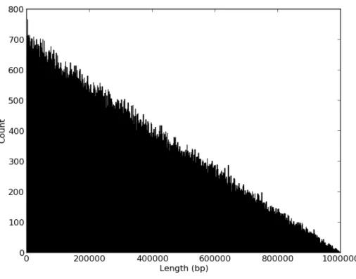
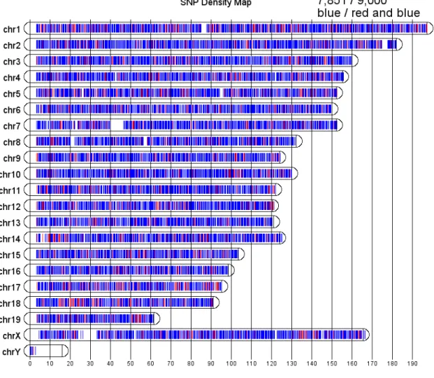
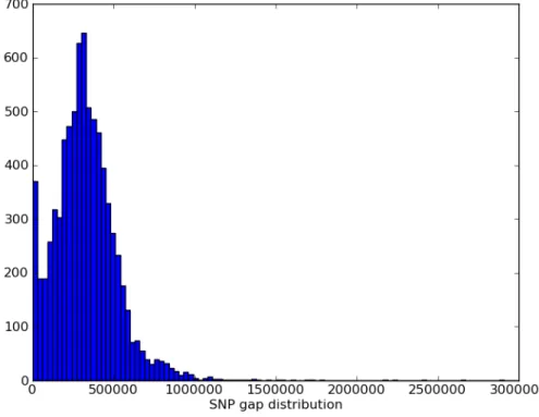
Of the original 9,000 SNPs selected, 7,851 were converted and placed on the Illumina In-finium platform (see Figure 4.2). The SNP markers have an average spacing of 325Kb (SD 191Kb); the distribution of the gaps between consecutive SNPs is shown in Figure 4.3. In geno-typing array design, it is fairly typical that some of the SNPs will not be included on the final array for various reasons. Illumina guarantees a success rate of converting SNPs in the design file to beads in the final array of at least 80%. Therefore, the conversion rate of 87% on MUGA was acceptable.
it was observed that many SNPs had unexpected intensity clusters outside the traditional AA, BB, or AB clusters. Many of these additional clusters are believed to be caused by previously unannotated SNPs within the probe sequence and with the most recently published SNPs from the Sanger Institute[30, 63], this hypothesis was confirmed. The final distribution of included SNPs can be seen in blue in Figure 4.2.
4.1.3 Samples Run on MUGA
Due to the CC founders’ genetic diversity and MUGA’s maximally informative design, MUGA’s utility extends beyond CC animals. To date, 8,265 samples have been genotyped on MUGA, including a large number of mice from the Collaborative Cross (CC), the Diversity Out-bred population (DO)[55], mice from the Mutant Mouse Regional Resource Centers (MMRRC), and wild mice. MUGA’s design allows for accurate ancestry inference of not only mice from developing CC lines but also mice with non-CC ancestors, such as those from the MMRRC repository. MUGA and its accompanying multiallelic genotyping algorithm provide a versatile and low-cost genotyping platform for laboratory mice from the CC population and beyond.
Included in the 8,265 samples genotyped on MUGA were eight copies of each CC founder, at least two copies of all viable F1 crosses between the CC founders, and 1,833 CC samples genotyped at various stages of inbreeding. There were also about 1,100 DO mice as well as some F2 crosses of inbred strains, congenics, consomics and wild mice. Performance tests were done on MUGA using a panel of controls to ensure that it was producing quality genotype calls.
4.1.4 Performance on MUGA
Sample 1 Sample 2 N=N H=H A=A # Discordant Calls
A/Jm111 A/J 127 91 7595 41
C57BL/6J C57BL/6J 30 87 7612 125
129S1/SvImJm212 129S1/SvImJ 145 75 7581 53 NZO/HlLtJ NZO/HlLtJm51 162 80 7572 40 CAST/EiJm42 CAST/EiJ 282 93 7398 81 PWK/PhJ-F11 PWK/PhJm175-C08 291 95 7368 100 WSB/EiJ-H06 WSB/EiJ-F09 168 85 7555 46 WSBxPWKf003 WSBxPWKm001 108 2737 4841 168 NODxPWKm004 NODxPWKm003 112 3438 4286 18 CASTxWSBf015 CASTxWSBm001 107 2678 4888 181
CASTxAJm005 CASTxAJm005 90 3426 4306 32 AJxPWKm006 AJxPWKf001 90 3430 4081 253 129xPWK037m 129xPWK 040F 85 3333 4124 312
Table 4.1: Comparison of biological replicate samples run on MUGA, where N=N depicts the number of times both samples had an N call at the same SNP, H=H depicts number of times both samples had an H call at the same SNP, A=A depicts the number of times the pair of samples had the same allele call (A, T, C, or G) at a particular SNP, and # of Discordant Calls depicts the total number of SNPs for which the two samples received different genotype calls.
of heterozygous calls and very high concordance between the two samples. The remaining sam-ples in the table are F1s (first generation cross between two inbreds). One would expect these samples to have a high number of heterozygous calls but still have high concordance between the samples. Over the entire table, there is 98.6% concordance among biological replicates, and if one only considers inbred concordance where the genotype call is an A, T, C, or G and that both samples tested had the same call, there is 95.8% concordance.
The next performance test performed on MUGA was testing how consistent F1 genotype calls were with the founder calls. Overall, it was found that the F1 genotype was 91.9% concor-dant with their founder parentals. Statistics were also collected on individual SNPs and any SNP that was found to be underperforming (getting N for all samples) was flagged in the database.
Array # SNPs Avg. Entropy Avg. bits per SNP MUGA 7851 0.75555 0.31077
Sanger 13457 0.80189 0.18622 MDA 550000 0.56828 0.081011
Table 4.2: Entropy scores for micro-array comparison. The Avg. Entropy column represents the average entropy per SNP, while the inverse of the Avg. bits per SNP shows the average number of SNPs it took to differentiate among all eight founders.
genotyping arrays. Based on the founder genotypes of the eight CC founders, it was determined that when strictly using genotype calls, 1,426 of the 7,851 SNPs on MUGA have an entropy score of 0 (no information content in terms of founder assignment). However, by using the intensities of the probes rather than the genotype calls, this entropy score can be much improved[25].
entropy scores than the typical biallelic SNP shown in (a), since if genotypes alone were used in (c), then there are only three possible calls (A, G, or H, since N calls are ignored)), but if intensity clusters are utilized, then five calls are possible[25].
In comparing entropy scores of genotyping arrays, only the genotype calls of the founder mice were used so that each array had the same possible information. The genotype information for the eight CC founders was obtained for the Sanger array [52] with 13,457 SNPs on it, as well as the Mouse Diversity Array(MDA)[64] with about 550,000 SNPs. Table 4.2 shows the calculated entropy scores for each of these arrays as well as MUGA. The Avg. Entropy column represents the average entropy per SNP, while Avg. bits per SNP shows the average number of SNPs it took to differentiate among all eight founders. To calculate this value, I divided three (the minimum number of SNPs with which it is possible to differentiate among all eight foundes) by the actual number of SNPs it took to create eight unique haplotypes. This number was then averaged over all sliding windows of the genome and shown in Table 4.2.
4.2 MegaMUGA
A second generation genotyping microarray, MegaMUGA, is also built on the Illumina Infinium platform and was designed to expand the number of markers and versatility of the suc-cessful Mouse Universal Genotyping Array (MUGA). It extends MUGA from 7.8K to 77.8K markers, and includes all MUGA markers as a subset. There are three types of probes on Mega-MUGA. In addition to traditional SNP probes, a second probe type for tracking known structural variants (insertions, deletions and duplications) has been introduced. A third probe type was designed to detect the presence of sequences present only in genetically engineered mice (GEM) (Cre, Luciferase, etc). MegaMUGA was designed to not only optimize the identification of founder contribution and detection of residual heterozygosity among CC strains at any stage of inbreeding, it was also designed to correctly identify the founder pairs present in areas of residual heterozygosity.
The vast majority of MegaMUGA probes ascertain traditional biallelic SNPs. SNPs were selected to be distributed across the entire genome including the mitochondria and the Y chro-mosome with an average spacing of 33 Kb. For the autosomes, these probes were distributed as evenly as possible based on a new linkage map[35] for the mouse with a slight excess of probes in the telomeric regions to facilitate detection of recombination events in these regions. SNPs were selected to be informative in most mouse populations (including wild mice and multiple Mus species) with a special emphasis for markers that are informative in the CC and DO populations.
4.2.1 Design
for GEM, 58 were selected for a chromosome evolution project, and 14 were selected for an X-inactivation mapping experiment [12]. To work well with the Illumina Infinium technology, these SNPs were all selected to not have any off-target variations within 50 base pair on at least one side. Also, the 49-mer either immediately preceding or following the SNPs must be unique and not occur elsewhere in the genome. All SNPs were also selected to include as few markers as possible that segregate beteween C/G or A/T alleles. This was done since as described in the MUGA section above, the technology used in Illumina genotyping arrays requires two beads to be developed to correctly differentiate between the aforementioned allele combinations. This means that a single SNP would cost two beads, so that less locations in the genome could be genotyped overall. In some regions of the genome, there were no alternative SNPs. Therefore, the final design of the array includes about 200 of these two-bead allele combination SNPs.
Of the 65,000 CC/DO SNPs, about 60,000 SNPs were selected to be uniformly distributed by recombination events over all autosomes and Chromosome X. About 20 invariants in the PAR region were included, as well as 45 SNPs on Chromosome Y, and 31 SNPs on the mitochrondria. The remaining SNPs were distributed in and beyond the last interval of each chromosome to obtain better resolution in a known high recombination area. Unlike in MUGA, the bin sizes for selecting SNPs are not uniform by genomic distance. Instead, the bin sizes were determined by using a mouse recombination map[35] so that the genome is binned into intervals with like-sized number of recombinations. To obtain this information, a series of plots were made, as shown in Figure 4.5, and it was determined that in order to choose 60,000 SNPs this way, 2.75 SNPs should be chosen per recombination (using only recombinations that were less than 25% of the length of the chromosome). The midpoints of the recombinations were used to determine the final bins to be used for SNP selection.
within each bin, SNPs with the same strain diversity pattern (SDP) were binned together. We looked at each chromosome in 5-bin sliding windows and used a dynamic programming algo-rithm to find one SDP in each interval that maximized the number of founder/F1 combinations that could be distinguised. The sliding window size was set to five since five SNPs is the fewest number that could potentially differentiate among all thirty-six founder and F1 combinations. Since all possible paths in the solution can increase exponentially, the possible solutions were pruned at each step. Occasionally a bin did not contain one of the eight candidate SDPs, which created a penalty for this path. Once the number of penalities along a particular path exceeded some threshold above the current best path, it was pruned. While this greedy pruning metric may not have produced the optimal path, it was able to produce a reasonable path in a short time period. As previously mentioned, the telomeres of chromosomes are very recombination rich, so therefore an additional 500 SNPs were selected at the ends of each chromosome in and be-yond the last interval found for each chromosome. These SNPs were selected in the same sliding window fashion as described above.
4.2.2 Samples Run on MegaMUGA
In total, more than 6,600 samples have been genotyped on MegaMUGA. Of these samples, eight copies of each CC founder were genotyped, as well as all viable F1 crosses betweeen the CC founders. There were also 462 CC samples genotyped at various stages of inbreeding, as well as a number of DO mice, F2 crosses of inbred strains, congenics, consomics, and wild mice.
4.2.3 Performance on MegaMUGA
As with MUGA, similar performance tests were run to ensure the quality of the SNP geno-typing calls. The first performance test was to compare the results from biological replicates to ensure that MegaMUGA was producing similar genotype calls on a per SNP basis. Table 4.3 shows the results of these comparisons for fifteen pairs of biological replicates. The first eight pairs in this table are inbred animals for which one would expect a low number of heterozygous calls and very high concordance between the two replicate samples. The remaining samples in the table are F1s (first generation cross between two inbreds). One would expect these samples to have a high number of heterozygous calls but still have high concordance between the replicate samples. Over the entire table, there is 98.9% concordance among biological replicates, and if one only considers inbred concordance where the genotype call is an A, T, C, or G (where A=A) and both samples have the same call, there is 96.2% concordance. The consistency of the F1 genotype calls with the founder calls was also tested. Overall, it was found that the F1 genotype was 95.2% concordant with their founder parentals. Statistics were also collected on individual SNPs and any SNP that was found to be underperforming (getting N for all samples) was flagged in the database.
4.3 Conclusion
Sample 1 Sample 2 N=N H=H A=A # Discordant 129S1/SvImJm1314 129S1/SvImJm35370 2194 237 75149 228
A/Jm0111 A/Jm0417 2196 242 75197 173
C57BL/6Jm1957 C57BL/6Jm36826 2109 246 75273 180 CAST/EiJm0042 CAST/EiJm0538 2807 208 74395 398 NOD/ShiLtJm0150 NOD/ShiLtJm1214 2212 214 75176 206 NZO/HILtJm0051 NZO/HILtJm0591 2217 225 75029 337 PWK/PhJm0175 PWK/PhJm1090 2749 191 74456 412 WSB/EiJm0993 WSB/EiJm1345 2303 208 73968 1329 (129S1xB6)F1f15916 (129S1xB6)F1m15914 2045 23889 51071 803 (129S1xPWK)F1f040 (129S1xPWK)F1m037 2105 37458 36567 1678
![Figure 2.3: Diversity Outbred (DO) breeding explanation[55].](https://thumb-us.123doks.com/thumbv2/123dok_us/8240955.2184097/30.918.241.704.125.477/figure-diversity-outbred-do-breeding-explanation.webp)