4775.pdf

(1)

A

n

E

xamination of

I

nitial

C

ondition

S

pecification in the

S

tructural

E

quations

M

odeling

F

ramework

Diane Losardo

A dissertation submitted to the faculty of the University of North Carolina at Chapel Hill in partial fulfillment of the requirements for the degree of Doctor of Philosophy in the Department of Psychology (Quantitative).

Chapel Hill 2012

Approved by

Sy-Miin Chow, Ph.D.

Patrick J. Curran, Ph.D.

(2)

c

2012

Diane Losardo

(3)

ABSTRACT

DIANE LOSARDO: An Examination of Initial Condition Specification in the Structural Equations Modeling Framework

(Under the direction of Sy-Miin Chow)

A challenge when estimating time series models is deciding how to correctly

specify an initial condition distribution, which describes the process prior to the first

sampled observation. For example, the process may have started in the distant past,

started exactly at the first observation point, or displayed a different structure before

the first time point was collected. Time series models may be estimated within the

structural equations modeling (SEM) framework (Browne & Nesselroade, 2005), and

while some psychological research has focused on the issue of initial condition

spec-ification (e.g., Du Toit & Browne, 2007; Chow, Ho., Hamaker, & Dolan, 2010; Oud,

Bercken, & Essers, 1990), a thorough examination of the consequences of using a

misspecified initial condition distribution has not been conducted. As the number of

time points increases, the consequences of a misspecified initial condition become less

severe (i.e., parameter estimates and state estimates are not affected as noticeably, see

Oud et al., 1990). If a process is not stationary (i.e., does not have the same mean and

covariance structure over time), then conventional methods for initial condition

spec-ification may not be appropriate (De Jong, 1991; Harvey, 1991). Proper methods for

such cases have been developed in the state-space literature (De Jong, 1991;

Koop-man, 1997). In this thesis I conducted a systematic examination comparing initial

condition specifications for time series models estimated within the SEM framework.

For stationary models, I considered three approaches, including (1) a model-implied

(4)

spec-proach (De Jong, 1991), which consists of augmenting the standard Kalman filter (KF)

with computational products associated with nonstationary portions of the model, a

modification by Koopman (1997), who developed an exact initial KF approach which

removes the reliance of the filtering equations on the nonstationary portions, and

a large κ approximation which is widely used in the time series literature but may

lead to numerical inaccuracies. A Monte Carlo simulation was conducted to

exam-ine parameter and state estimate recovery given different types of initial condition

specification for both intensive repeated measures data and panel data. Finally, each

initial condition specification was estimated using an empirical data set.

Results suggest that, when the process is nonstationary and true initial condition

is diffuse, the de Jong initial condition approach leads to proper point and standard

error estimates with fewer numerical difficulties when compared to the other

ap-proaches. However, the Koopman and free-parameter approaches also performed

well, but exhibited more severe computational problems in the estimation process,

leading to convergence problems and biased point estimates of the variance

param-eters. Furthermore, results illustrate how using different initial condition

specifica-tions with real data may lead to different point and standard error estimates and thus

different substantive conclusions. Implications of results and recommendations for

(5)

(6)

ACKNOWLEDGEMENTS

I wish to thank everyone who has helped and supported me throughout this

dissertation process. First, I thank my advisor, Sy-Miin Chow, for her perpetual

guidance, support, and encouragment. I am grateful for the many hours she spent

with me explaining difficult concepts and providing me with useful resources while

allowing me to pursue research on such interesting topics.

I thank Patrick Curran, who provided me with the foundational knowledge for

understanding key concepts in psychometrics. His mentorship was valuable not only

in the process of my dissertation, but also in preparing me academically and mentally

for the completion of such a task.

I also thank the rest of my dissertation committee members - Stephen du Toit,

Andrea Hussong, and Bud MacCallum - for their helpful suggestions and creative

ideas throughout this process. I thank all members of the L.L. Thurstone lab for

providing me with such a great atmosphere for learning. I thank the former

mem-bers of the Curran Army, Daniel, Jim, and Taehun, for providing me with so much

knowledge and laughter.

I thank my family for support and encouragement throughout the years of this

process. I am grateful for my friends who kept me sane when times were tough

- thank you Kristi, Ben, Allison, Dana, Jolynn, Susan, Ellen, Andrea, and last but

not least, John, whose support in the last few months leading up to my dissertation

defense was invaluable.

(7)

CHAPTER

1 Introduction . . . 1

1.1 Stationary vs. Nonstationary Processes . . . 4

1.2 Initial Condition and Stationarity. . . 12

1.3 State-Space Modeling Framework . . . 16

1.4 Structural Equation Modeling Framework . . . 20

1.5 Similarities Between SEM and State-Space Modeling Frameworks . . . 21

1.6 Technical Detail of Initial Condition Specifica-tion in the SEM Framework . . . 25

1.7 Technical Detail of Initial Condition Specifica-tion in the State-Space Modeling Framework . . . 34

1.8 Examples of Initial Condition Specification in the Literature . . . 48

1.9 Current Investigation . . . 53

2 Methods . . . 55

2.1 Models . . . 57

2.2 Initial Condition Specification . . . 66

2.3 Software Packages . . . 72

(8)

2.5 Outcome Measures . . . 73

2.6 Hypotheses . . . 75

3 Results . . . 78

3.1 Model Convergence Issues . . . 79

3.2 Stationary PFA . . . 83

3.3 Summary of Stationary Results . . . 92

3.4 Nonstationary PFA . . . 93

3.5 Mildly Nonstationary PFA . . . 96

3.6 Moderately Nonstationary PFA . . . 102

3.7 Summary of Nonstationary Results . . . 108

3.8 General Simulation Conclusions . . . 109

3.9 Results Removing Boundary Cases . . . 110

3.10 Empirical Example . . . 126

4 Discussion . . . 135

4.1 Recommendations for Practice . . . 139

4.2 Limitations and Future Directions . . . 142

5 Appendix A . . . 146

6 Appendix B . . . 170

(9)

LIST OF TABLES

1.1 Kalman Filter Comparisons . . . 47

2.1 Summary of Simulation Design . . . 56

2.2 Summary of Initial Condition Specifications . . . 65

2.3 Initial Condition Specifications for Model 1:

Station-ary PFA(1,0) Model . . . 69

2.4 Initial Condition Specifications for Model 2:

Non-stationary PFA(1,0) . . . 70

2.5 True vs. Fitted Initial Condition Specifications . . . 71

3.1 Rates of Convergence to a Proper Solution, AIC and

BIC Model Selection, Latent Variable Recovery, and

Average Total Time Obtained from Stationary PFA Model. . . 81

BIC Model Selection, Latent Variable Recovery, and Average Total Time Obtained from Nonstationary

PFA Model Mild Nonstationarity. . . 94

BIC Model Selection, Latent Variable Recovery, and Average Total Time Obtained from Nonstationary

PFA Model with Moderate Nonstationarity. . . 95

BIC Model Selection, Latent Variable Recovery, and Average Total Time Obtained from Stationary PFA

Model Removing Boundary Cases. . . 111

BIC Model Selection, Latent Variable Recovery, and Average Total Time Obtained from Nonstationary PFA Model Mild Nonstationarity Removing

(10)

3.6 Rates of Convergence to a Proper Solution, AIC and BIC Model Selection, Latent Variable Recovery, and Average Total Time Obtained from Nonstationary PFA Model with Moderate Nonstationarity

Remov-ing Boundary Cases. . . 113

3.7 Summary Statistics for Manifest Variables of

Empir-ical Example . . . 127

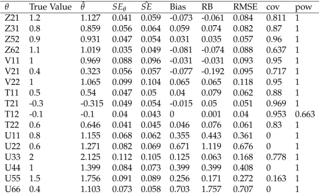
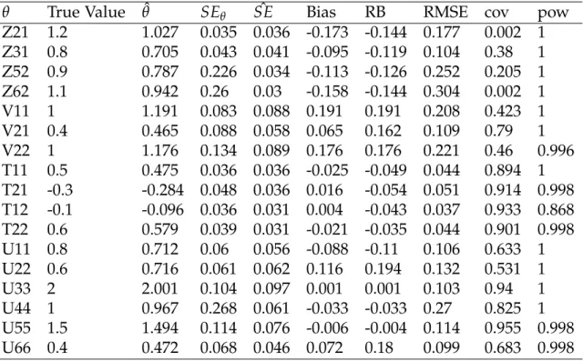
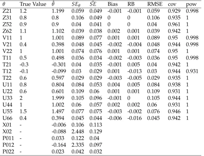
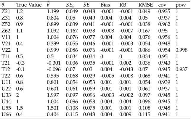
3.8 Parameter Estimates and Standard Errors for

PFA(1,0) Empirical Example . . . 129

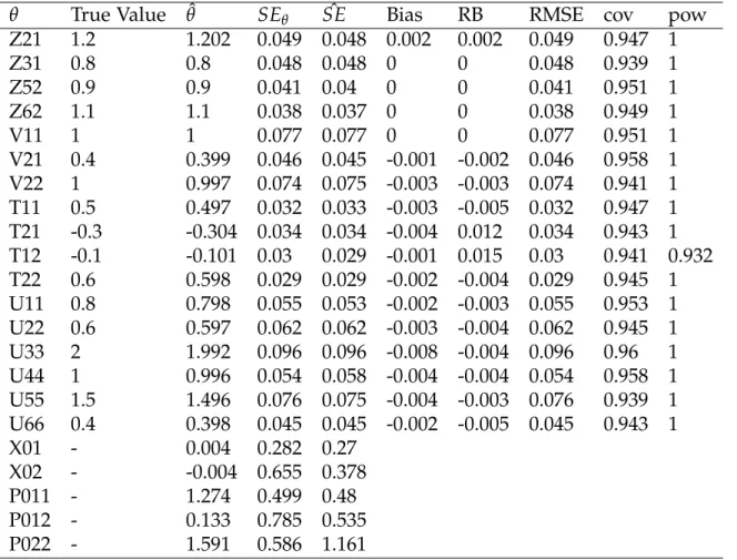
5.1 Stationary PFA Results: True IC: Model Implied,

Fit-ted IC: Model Implied, N=20, T=50 . . . 146

Fit-ted IC: Free Parameter, N=20, T=50 . . . 147

Fit-ted IC: Null, N=20, T=50 . . . 148

Fit-ted IC: deJong DKF, N=20, T=50 . . . 148

Fit-ted IC: Koopman exact initial KF, N=20, T=50 . . . 149

Fit-ted IC: Large κ, N=20, T=50 . . . 149

5.7 Simulation Results: True IC: Model Implied, Fitted

IC: Model Implied, N=200, T=5 . . . 150

IC: Free Parameter, N=200, T=5 . . . 151

IC: Null, N=200, T=5 . . . 152

IC: deJong DKF, N=200, T=5 . . . 152

IC: Koopman exact initial KF, N=200, T=5 . . . 153

IC: Largeκ, N=200, T=5 . . . 153

(11)

5.14 Stationary PFA Results: True IC: Null, Fitted IC:

Free Parameter, N=20, T=50 . . . 155

Null, N=20, T=50 . . . 156

de-Jong DKF, N=20, T=50 . . . 156

Koopman exact initial KF, N=20, T=50 . . . 157

Large κ, N=20, T=50 . . . 157

Model Implied, N=200, T=5 . . . 158

Free Parameter, N=200, T=5 . . . 159

Null, N=200, T=5 . . . 160

de-Jong DKF, N=200, T=5 . . . 160

Large κ, N=200, T=5 . . . 161

5.25 Stationary PFA Results: True IC: Free Parameter,

Fitted IC: Model Implied, N=20, T=50 . . . 162

Fitted IC: Free Parameter, N=20, T=50 . . . 163

Fitted IC: Null, N=20, T=50 . . . 164

Fitted IC: deJong DKF, N=20, T=50 . . . 164

Fitted IC: Koopman exact initial KF, N=20, T=50 . . . 165

(12)

Fitted IC: Model Implied, N=200, T=5 . . . 166

Fitted IC: Free Parameter, N=200, T=5 . . . 167

Fitted IC: Null, N=200, T=5 . . . 168

Fitted IC: deJong DKF, N=200, T=5 . . . 168

Fitted IC: Koopman exact initial KF, N=200, T=5 . . . 169

Fitted IC: Large κ, N=200, T=5 . . . 169

6.1 Nonstationary PFA Results: True IC: Null, Fitted IC:

Free Parameter, N=20, T=50, Mild Nonstationarity . . . 170

Null, N=20, T=50, Mild Nonstationarity . . . 171

deJong DKF, N=20, T=50, Mild Nonstationarity . . . 171

Koopman exact initial KF, N=20, T=50, Mild Nonstationarity . . . 172

Large κ, N=20, T=50, Mild Nonstationarity . . . 172

Free Parameter, N=200, T=5, Moderate Nonstationarity . . . 173

Null, N=200, T=5, Moderate Nonstationarity . . . 174

deJong DKF, N=200, T=5, Moderate Nonstationarity . . . 174

Koopman exact initial KF, N=200, T=5, Moderate Nonstationarity . . . 175

Large κ, N=200, T=5, Moderate Nonstationarity . . . 175

(13)

Null, N=200, T=5, Mild Nonstationarity . . . 177

deJong DKF, N=200, T=5, Mild Nonstationarity . . . 177

Koopman exact initial KF, N=200, T=5, Mild Nonstationarity . . . 178

Large κ, N=200, T=5, Mild Nonstationarity . . . 178

6.16 Nonstationary PFA Results: True IC: Free Param-eter, Fitted IC: Free ParamParam-eter, N=20, T=50, Mild

Nonstationarity . . . 179

6.17 Nonstationary PFA Results: True IC: Free

Parame-ter, Fitted IC: Null, N=20, T=50, Mild Nonstationarity . . . 180

6.18 Nonstationary PFA Results: True IC: Free Parame-ter, Fitted IC: deJong DKF, N=20, T=50, Mild

Non-stationarity . . . 180

6.19 Nonstationary PFA Results: True IC: Free Parame-ter, Fitted IC: Koopman exact initial KF, N=20, T=50,

Mild Nonstationarity . . . 181

Parame-ter, Fitted IC: Large κ, N=20, T=50, Mild

Nonsta-tionarity . . . 181

6.21 Nonstationary PFA Results: True IC: Free Parame-ter, Fitted IC: Free ParameParame-ter, N=200, T=5, Moderate

6.22 Nonstationary PFA Results: True IC: Free Parame-ter, Fitted IC: Null, N=200, T=5, Moderate

6.23 Nonstationary PFA Results: True IC: Free Parame-ter, Fitted IC: deJong DKF, N=200, T=5, Moderate

Moderate Nonstationarity . . . 184

Parame-ter, Fitted IC: Large κ, N=200, T=5, Moderate

(14)

6.26 Nonstationary PFA Results: True IC: Free Param-eter, Fitted IC: Free ParamParam-eter, N=200, T=5, Mild

Parame-ter, Fitted IC: Null, N=200, T=5, Mild Nonstationarity . . . 186

6.28 Nonstationary PFA Results: True IC: Free Parame-ter, Fitted IC: deJong DKF, N=200, T=5, Mild

Mild Nonstationarity . . . 187

Parame-ter, Fitted IC: Large κ, N=200, T=5, Mild

6.31 Nonstationary PFA Results: True IC: Diffuse, Fitted

IC: Free Parameter, N=20, T=50, Mild Nonstationarity . . . 188

IC: Null, N=20, T=50, Mild Nonstationarity . . . 189

IC: deJong DKF, N=20, T=50, Mild Nonstationarity . . . 189

IC: Koopman exact initial KF, N=20, T=50, Mild Nonstationarity . . . 190

IC: Largeκ, N=20, T=50, Mild Nonstationarity . . . 190

6.36 Simulation Results: True IC: Diffuse, Fitted IC: Free

Parameter, N=200, T=5 . . . 191

6.37 Simulation Results: True IC: Diffuse, Fitted IC: Null,

N=200, T=5 . . . 192

6.38 Simulation Results: True IC: Diffuse, Fitted IC:

de-Jong DKF, N=200, T=5 . . . 192

(15)

6.42 Simulation Results: True IC: Diffuse, Fitted IC: Null,

N=200, T=5, Mild Nonstationarity . . . 195

de-Jong DKF, N=200, T=5, Mild Nonstationarity . . . 195

6.44 Simulation Results: True IC: Diffuse, Fitted IC: Koopman exact initial KF, N=200, T=5, Mild

(16)

LIST OF FIGURES

2.1 Time series plots of states for Model 1 (A), Model

2 with moderate nonstationarity (B), and Model 2 with mild nonstationarity. Time is displayed on the

x-axis. . . 61

2.2 Autocorrelation plots of states for one individual for

Model 1 (A), Model 2 with moderate nonstationar-ity (B), and Model 2 with mild nonstationarnonstationar-ity. Lag

is displayed on the x-axis. . . 62

2.3 Partial autocorrelation plots of states for one

indi-vidual for Model 1 (A), Model 2 with moderate non-stationarity (B), and Model 2 with mild

nonstation-arity. Lag is displayed on the x-axis. . . 63

3.1 Sample of typical outlier cases removed. The

free-parameter model is fitted to the moderately nonsta-tionary model using a diffuse true initial condition specification. The x-axis displays parameter

esti-mates of Z52, and the values displaying an absolute

value greater than 30 were removed. . . 82

3.2 Sample of typical cases hitting a boundary

condi-tion. The free-parameter model is fitted to the mod-erately nonstationary model using a diffuse true ini-tial condition specification. The x-axis displays

pa-rameter estimates of V22, and the values that are

very close to zero were removed for the second set

(17)

3.3 Absolute bias, coverage rates, calculated as the ab-solute difference from .95, abab-solute empirical

stan-dard errors ( ˆSD) minus estimated standard errors

(SEθ), calculated as abs(SEθ−SEˆ ), for the average of

(A)–(B) measurement parameters, (C)–(D) process noise parameters, and (E)–(F) time series parame-ters for the stationary PFA model simulated using the model-implied moments method as the true ini-tial condition specification. DKF=de Jong’s diffuse Kalman filter approach, EKF=Koopman’s exact

ini-tial Kalman filter approach. . . 87

3.4 Absolute bias, coverage rates, calculated as the

ab-solute difference from .95, abab-solute empirical

(A)–(B) measurement parameters, (C)–(D) process noise parameters, and (E)–(F) time series parame-ters for the stationary PFA model simulated using the free parameter moments method as the true

ini-tial condition specification. . . 89

(SEθ), calculated as abs(SEθ−SEˆ ), for the average of (A)–(B) measurement parameters, (C)–(D) process noise parameters, and (E)–(F) time series parame-ters for the stationary PFA model simulated using the null method as the true initial condition spec-ification. DKF=de Jong’s diffuse Kalman filter ap-proach, EKF=Koopman’s exact initial Kalman filter

approach. . . 91

(A)–(B) measurement parameters, (C)–(D) process noise parameters, and (E)–(F) time series parame-ters for the nonstationary PFA model simulated us-ing the free parameter moments method as the true initial condition specification with mildly nonsta-tionary population values. DKF=de Jong’s diffuse Kalman filter approach, EKF=Koopman’s exact

(18)

(SEθ), calculated as abs(SEθ −SEˆ ), for the average

of (A)–(B) measurement parameters, (C)–(D) pro-cess noise parameters, and (E)–(F) time series pa-rameters for the nonstationary PFA model simu-lated using the null method as the true initial con-dition specification with mildly nonstationary pop-ulation values. DKF=de Jong’s diffuse Kalman filter approach, EKF=Koopman’s exact initial Kalman

fil-ter approach. . . 99

(SEθ), calculated as abs(SEθ−SEˆ ), for the average of (A)–(B) measurement parameters, (C)–(D) process noise parameters, and (E)–(F) time series parame-ters for the nonstationary PFA model simulated us-ing the diffuse method as the true initial condition specification with mildly nonstationary population values. DKF=de Jong’s diffuse Kalman filter ap-proach, EKF=Koopman’s exact initial Kalman filter

approach. . . 101

(A)–(B) measurement parameters, (C)–(D) process noise parameters, and (E)–(F) time series parame-ters for the nonstationary PFA model simulated us-ing the free parameter moments method as the true initial condition specification with moderately non-stationary population values. DKF=de Jong’s dif-fuse Kalman filter approach, EKF=Koopman’s exact

(19)

(A)–(B) measurement parameters, (C)–(D) process noise parameters, and (E)–(F) time series param-eters for the nonstationary PFA model simulated using the null method as the true initial condition specification with moderately nonstationary popu-lation values. DKF=de Jong’s diffuse Kalman filter approach, EKF=Koopman’s exact initial Kalman

(SEθ), calculated as abs(SEθ−SEˆ ), for the average of (A)–(B) measurement parameters, (C)–(D) process noise parameters, and (E)–(F) time series parame-ters for the nonstationary PFA model simulated us-ing the diffuse method as the true initial condition specification with moderately nonstationary popu-lation values. DKF=de Jong’s diffuse Kalman filter approach, EKF=Koopman’s exact initial Kalman

(A)–(B) measurement parameters, (C)–(D) process noise parameters, and (E)–(F) time series parame-ters for the stationary PFA model simulated using the free parameter moments method as the true ini-tial condition specification. DKF=de Jong’s diffuse Kalman filter approach, EKF=Koopman’s exact

(20)

(A)–(B) measurement parameters, (C)–(D) process noise parameters, and (E)–(F) time series parame-ters for the stationary PFA model simulated using the null method as the true initial condition spec-ification. DKF=de Jong’s diffuse Kalman filter ap-proach, EKF=Koopman’s exact initial Kalman filter

approach. . . 118

(A)–(B) measurement parameters, (C)–(D) process noise parameters, and (E)–(F) time series parame-ters for the stationary PFA model simulated using the model-implied moments method as the true ini-tial condition specification. DKF=de Jong’s diffuse Kalman filter approach, EKF=Koopman’s exact

ini-tial Kalman filter approach. . . 119

(A)–(B) measurement parameters, (C)–(D) process noise parameters, and (E)–(F) time series parame-ters for the nonstationary PFA model simulated us-ing the free parameter moments method as the true initial condition specification with mildly nonsta-tionary population values. DKF=de Jong’s diffuse Kalman filter approach, EKF=Koopman’s exact

(21)

(SEθ), calculated as abs(SEθ −SEˆ ), for the average

of (A)–(B) measurement parameters, (C)–(D) pro-cess noise parameters, and (E)–(F) time series pa-rameters for the nonstationary PFA model simu-lated using the null method as the true initial con-dition specification with mildly nonstationary pop-ulation values. DKF=de Jong’s diffuse Kalman filter approach, EKF=Koopman’s exact initial Kalman

(SEθ), calculated as abs(SEθ−SEˆ ), for the average of (A)–(B) measurement parameters, (C)–(D) process noise parameters, and (E)–(F) time series parame-ters for the nonstationary PFA model simulated us-ing the diffuse method as the true initial condition specification with mildly nonstationary population values. DKF=de Jong’s diffuse Kalman filter ap-proach, EKF=Koopman’s exact initial Kalman filter

approach. . . 122

(A)–(B) measurement parameters, (C)–(D) process noise parameters, and (E)–(F) time series parame-ters for the nonstationary PFA model simulated us-ing the free parameter moments method as the true initial condition specification with moderately non-stationary population values. DKF=de Jong’s dif-fuse Kalman filter approach, EKF=Koopman’s exact

(22)

(A)–(B) measurement parameters, (C)–(D) process noise parameters, and (E)–(F) time series param-eters for the nonstationary PFA model simulated using the null method as the true initial condition specification with moderately nonstationary popu-lation values. DKF=de Jong’s diffuse Kalman filter approach, EKF=Koopman’s exact initial Kalman

(SEθ), calculated as abs(SEθ−SEˆ ), for the average of (A)–(B) measurement parameters, (C)–(D) process noise parameters, and (E)–(F) time series parame-ters for the nonstationary PFA model simulated us-ing the diffuse method as the true initial condition specification with moderately nonstationary popu-lation values. DKF=de Jong’s diffuse Kalman filter approach, EKF=Koopman’s exact initial Kalman

3.21 Comparison of parameter estimates (A) and stan-dard errors (B) for the factor loading, process noise, and time series parameters, and parameter esti-mates (C) and standard errors (D) for the mea-surement error variances, produced from the null,

free parameter, de Jong, Koopman, and large κ

ap-proaches when applied to the empirical data set. Because the de Jong and Koopman approaches pro-duced identical estimates to the 7th decimal place,

they are grouped together . . . 131

3.22 Comparison of estimated latent variable scores for the null, free-parameter, de Jong and Koopman, and

large κ approaches when applied to the empirical

(23)

esti-CHAPTER 1

Introduction

While initial condition specification has not been extensively discussed within

the psychological literature, there are both methodological and substantive reasons

as to why it is an important topic to consider. Generally speaking, an initial

condi-tion distribucondi-tion describes the structure of a process before the first observation was

collected, or right on the first occasion. As an example, consider a situation where

a psychologist has collected longitudinal data for a given time frame. A model may

then be fit to the data in hopes of uncovering and understanding some

underly-ing process. However, it is very possible that the process has started in the distant

past, and furthermore that the structure of the process was different before the first

collected data point. It is also possible that the overall process displays differing

structures as a function of time, thus rendering it difficult to discern what the initial

condition process was.

From a substantive viewpoint, the role of initial condition in certain

psycholog-ical theories plays a major part. Several psychologpsycholog-ical theories concerning initial

condition have been proposed within the context of chaotic processes that are highly

nonlinear in nature, but are actually deterministic (i.e., a process that can be

per-fectly predicted given current and previous information) (see Robertson & Combs,

1995). Such a process has been hypothesized to exist in several areas of psychology,

(24)

and developmental psychology (Ayers, 1997). One element of a chaotic process, as

applied to explain a psychological process, is the idea that a process is very sensitive

to its initial condition status. Consequently, small changes in initial condition may

produce large effects over time. As an example, Gottschalk, Bauer, and Whybrow

(1995) found evidence indicating that long-term mood variations for both bi-polar

patients and normal patients are not periodic in nature, and may display some form

of chaotic behavior.

Some theories in developmental psychology posit that early childhood events,

which may be loosely thought of as initial conditions for a given individual, have a

significant and long-lasting effect on an individual’s trajectory into adulthood.

Clas-sic examples include attachment theory (Bowlby, 1982), social-cognitive theories (e.g.,

Vygotsky, 1978), and social-cognitive learning theory (Bandura, 1986). As cognitive

growth tends to be rapid during early childhood, any environmental or biological

influences may be more pronounced and affect the eventual progression to a more

stable cognitive style (Sternberg, 1999). An individual’s social development and

so-cial engagement have also been hypothesized to display rapid growth at early ages,

and thus be sensitive to any internal or external events that eventually shape the

per-son’s more stable social behavior. Early psychological trauma, such as child

maltreat-ment, may have a long term effect on a child’s functioning with respect to both brain

development (Cicchetti & Tucker, 1994) and psychological functioning (Maughan &

Cicchetti, 2002). For example, Greenberg, Kusche, and Spelz (1991) discussed how

children’s early exposure to either witnessing or being victims of violence along with

a display of negative affect may hinder a child’s ability to effectively manage and

process emotions. This may, in turn, lead to a larger risk of psychopathology in

adulthood. In the substance use literature, early engagement in problem behaviors

(25)

Costa, 1991; Zucker, Chermack, & Curran, 2000).

Such theories indicate that the role of initial condition in psychological research is

important to consider and may help shape a developmental pathway into adulthood.

It is not always the case, however, that a researcher will know how to characterize

the initial condition distribution. Consider the case where a researcher collects data

on a sample of individuals with a certain anxiety disorder. One measured variable

may be the degree to which a person displays a symptom of anxiety. If this variable

is tracked over the course of a few weeks, a trajectory of anxiety levels for the

sam-pled individuals will be revealed. However, it is unlikely that the given individuals

began to display such a process at the exact time the first data point was collected.

This process may have started long before the data were collected, and may even

have displayed a different structure beforehand. In other words, the initial condition

distribution may be characterized differently than the distribution of the process for

the sampled time frame.

One way psychologists have attempted to explain initial condition status is by

introducing covariates, such as gender, socioeconomic status, and age, to help explain

interindividual differences in initial condition. One example is adding covariates into

a growth curve model to explain interindividual differences in intercept. However,

as stated, this prior knowledge is not always available or exhaustive. If there is no

precise information available researchers may have to resort to other specifications

of initial condition. In this thesis, I consider some of these possible specifications.

I describe different procedures that have been used for initializing a process and

evaluate a set of procedures for more accurately specifying initial condition, with a

focus on types of data that are commonly collected in psychological research. I first

describe stationary and nonstationary processes in more detail as such processes are

(26)

1.1 Stationary vs. Nonstationary Processes

To begin, I will introduce the more technical definitions that describe and

catego-rize a process. Specifically, processes may be generally described as either stationary

or nonstationary (Chatfield, 2004; Hamilton, 1994; Shumway & Stoffer, 2006; Wei,

1990), which are terms that arise from the time series literature. Broadly speaking,

a stationary process implies that the statistical properties, including mean, variance,

and higher order moments, of a process do not change over time regardless of when

data were sampled. A nonstationary process, in contrast, may display a different

process depending on a given time frame. This includes time frames that occurred

before a given data point was sampled. Depending on the type of stationarity,

differ-ent initial condition distributions will be needed to properly specify the model and

to ensure that accurate latent variable scores and parameter estimates are obtained.

Time series processes and stationarity. To more extensively describe the stationarity

of a process, I will illustrate how it is explained within the context of time series

processes. In general, time series models allow for the examination of the relations

between series of random variables indexed by time (Chatfield, 2004; Hamilton, 1994;

Shumway & Stoffer, 2006; Wei, 1990). Specifically, a multiple-subject time series may

be represented by the following equation:

xit = git+vit (1.1)

where xit represent outcome variables for a given person i (i = 1, 2 . . .N) and time

point t (t = 1, 2 . . .T), git represents a time series process, such as an autoregressive

(AR) or moving average (MA) process, and vit represents noise or uncertainties in

the change process, such as a white noise process (i.e., a process of uncorrelated

(27)

Browne and Nesselroade (2005) referred to git as the process variables andvitas

a series of random shocks (i.e.,”dynamic noise,” often assumed to be white noise).

The process variables are those that are changing over time, while the random shock

variables are forces that cause uncertainties in the process variables. Two examples

of time series processes are an AR(p) process and an MA(q) process

AR(p): xit =α1xi,t−1+α2xi,t−2+...+αpxi,t−p+vit vit∼ N(0,σv2) (1.2)

MA(q): xit =β1vi,t−1+β2vi,t−2+...+βqvi,t−q+vit vit∼ N(0,σv2) (1.3)

where the xit variables represent the process variables and the vitvariables represent

the random shocks that are uncorrelated with each other over time and distributed

normally with a mean zero and varianceσv2.

Multiple-subject time series models may be extended to includenx-vector

(multi-variate) autoregression with moving average (VARMA) processes (Shumway &

Stof-fer, 2006), where nx equals the number of x variables. In this case, the model is

formulated as

xit = p

∑

r=1

Arxi,t−1+

q

∑

j=1

Bjvi,t−j+vit (1.4)

wherexit represents a set ofnx×1 vectors of process variables,uitrepresents a set of

nx×1 vectors of random shock variables which are again normally distributed with

a mean vector of zero and covariance matrix Σv, A1, . . . ,Ap represent the nx×nx

autoregression weight matrices, andB1, . . . ,Bq represent thenx×nxmoving average

weight matrices. There are now a total of N×T×nx observations. To technically

define a stationary process, consider the backshift operator B,

(28)

such that the VARMA process may be re-written as

(I−A1B1−. . .−ApBp)xit =vit. (1.6)

Then, the process is mathematically defined as stationary if the roots of the

determi-nant of

(I−A₁B1−. . .−ApBp) (1.7)

lie outside of the unit circle (i.e., all roots have a modulus, or absolute value, greater

than 1, Ltkepohl, 1993). This model may be particularly attractive to psychologists as

they allow for a focus on understanding intra-individual (i.e., within person) changes

while still retaining a multivariate orientation.

As the variables are dependent on each other with respect to time, in order to

fully understand the concept of stationarity we must first understand the

autoco-variance function of a process. This function is a measure of the linear dependence

between two observations from the same time series, measured as

Γ(s,t) = E[(xi,s−µs)(xi,t−µt)] (1.8)

wheres−trepresents an arbitrary time lag. The smoother a time series is, the larger

the autocovariance value will be. If the autocovariance function is zero, then there

exists no linear dependency amongx_i_,_s andx_i_,_t, and the series will be choppier. Note

that this function applies to all individuals within the time series.

Inherent within time series is the idea that there is some regularity to be modeled

plus some noise, or ”error.” This regularity is tested by making use of the concept of

(29)

be formally expressed in mathematical terms by considering processes that display

strong stationarity, weak stationarity, or nonstationarity.

Strong stationarity asserts that the probabilistic behavior of every set of

observa-tions remains the same when there is an arbitrary shift in time, expressed as t+h.

Formally, this states that every set of observations x_i₁,x_i₂, . . . ,x_ik will have the same

joint statistical distribution as a time shifted setx_i_,1+h,xi,2+h, . . . ,xi,k+h. Thus,

P(xi1 ≤c1, . . . ,xik ≤ck) = P(xi,1+h ≤c1, . . . ,xi,k+h ≤ck) (1.9)

holds for all k=1, 2, . . ., all time pointst1,t2, . . . ,tk, all constantsc1,c2, . . . ,ck, and all

time shifts h = 0,±1,±2, . . .. This implies that the probability of observing a value

at a given time period is the same as the probability of observing the value at a later

or earlier time period. Also, the mean function does not change with time, so that

µt =µs =µfor allsandt. Any process that involves a mean change over time is then

not stationary. Additionally, the variance function, which is the autocovariance of a

variable with itself, does not change with time. The autocovariance of a stationary

process can be defined as:

Γ(s,t) = Γ(s+h,t+h) (1.10)

Thus, the covariance depends on the lag, or time difference between s and t, only

and not on the actual times. This strong stationarity incorporates all of the possible

distributions of a time series. Thus, not only are the first two moments stationary, but

all possible characteristics of the distribution, including higher-order moments. This

assumption is very strict and difficult to meet, especially in data commonly collected

in psychological research.

A more relaxed version of stationarity is termed weak stationarity. Instead of

making assumptions about the entire probability distribution, this version focuses on

(30)

across time points and the covariance structure depends only on the lag s−t, and given this lag remains constant over time. Also, if a process arises from a multivariate

normal distribution and is weakly stationary, it is considered to formally exhibit a

stationary process. To illustrate these points more concretely, I will now provide

examples of both stationary and nonstationary processes.

Examples of stationary processes. One example of a model with a stationary process is

an AR(1) model where |α1| <1. A psychological process that might align well with

this model could be an individual’s overall mood sampled daily over the course of

a few weeks. The model testifies that a person’s current mood is affected by his or

her mood on a previous day, and to a lesser extent by his or her mood two days ago,

and to an even lesser extent by his or her mood three days ago, and so forth. This

can be understood more precisely by examining the autocovariance function for an

AR(1) process, expressed as

σv2αs−t

1−α2. (1.11)

The numerator of this term expresses the AR(1) weight α as being raised to the

power of s−t, which represents a time lag. Thus, if |α1| <1, larger lags in time will

be characterized by an autocovariance closer to zero. In other words, the covariance

between any two observations is attenuated exponentially (i.e., decays) as the two

observations are further apart in time, either with (when −1 < α1 ≤ 0) or without

(when 0 ≤ α1 < 1) fluctuations. Thus, the linear dependence between a person’s

mood on, say, day 1 as compared to day 10 is lower than the linear dependence of a

person’s mood on day 1 as compared to day 3.

Another feature of a stationary AR(1) model where |α1| < 1 is that the random

(31)

uncertainties that may be different from day to day. For example, a person’s anxiety

may be affected today by a pop-quiz in his or her calculus class and tomorrow by

an unannounced visit from a family member. Still, the process is stationary in that

it ensures that large effects of a process variable will become less pronounced with

time instead of being intensified over time.

Another example of a stationary process is a MA(1) model, which is

mathemati-cally expressed as:

xit =β1vi,t−1+vit. (1.12)

In this model, the random shock variables for a given time point directly affect the

process variable for that time point but also directly affect the process variable for

the subsequent time point. A psychological process that might align well with this

model is one where random day-to-day environmental or external influences, such

as a rainy day or a pop quiz, are hypothesized to directly influence a person’s current

mood and also his or her mood the following day. However, the affect of the external

influence will be gone the third day.

This process has an expected value of zero, a variance of (1+β2)σ_v2 and an

autocovariance function of:

Γ(s,t) =

  

 

βσv2, if (s−t) = 1

0, if (s−t) >1

(1.13)

Thus, the process is stationary as time does not appear in any of these equations.

As discussed, however, not all processes are stationary. I will now discuss several

models that describe nonstationary processes.

Examples of nonstationary processes. A nonstationary process is one that allows the

(32)

an arbitrary shift in time. The process may become ”explosive” in the sense that the

effects of current process variables are magnified with time as opposed to decaying

with time. An example of this process is the random walk model, which has the

structure of an AR(1) process with α =1, expressed as

xit =xi,t−1+vit. (1.14)

In this model, the value of thexivariable at timetis the value of the xivariable at

timet−1 plus a random movement determined byvit. This process is non-stationary

as the variance of the random walk is equal totσv2, which increases without bound as

time increases. The autocovariance function is equal to min(s,t)σv2 and depends on

the particular time values, s and t, and not just the time lag s−t. Finally, the mean

function changes also changes with time. Another nonstationary process is a random

walk with drift model, which is expressed as

xit=ν+xi,t−1+vit (1.15)

where ν is a constant called the ”drift”, or stochastic trend. This process is

nonsta-tionary with respect to its mean structure, which is equal to νt. The mean of this

process, then, increases astincreases. This may be more clearly illustrated by

rewrit-ing the random walk with drift process as a cumulative sum of the random shock

variables, expressed as

xit =νt+

T

∑

j=1

vij. (1.16)

Here we can see that the past influences of the process accumulate over time and

(33)

time, this person might become more and more emotionally unstable, as the original

effects of instability do not diminish with time, but rather accumulate with time.

Also, as time increases, so does the variability of a person’s emotional state, as the

person becomes more and more unstable.

Another model that describes a nonstationary process is the latent curve model

(LCM; Meredith & Tisak, 1990), which is a longitudinal model estimated within

the structural equation modeling (SEM; see Bollen, 1989) framework. This model

describes the process via a set of latent factors that are theorized to have given rise

to set of repeated measures. For example, if a linear trend is hypothesized, the

model implies that the process may be explained in part by an intercept latent factor

(i.e., initial starting point) and linear slope latent factor. Furthermore, individual

differences may be captured by allowing the two latent factors to have a group mean

plus variability around this group mean. A larger degree of variability indicates that

there are more individual differences in either the intercept or slope.

While psychologists sometimes implement such models, they may be unaware

that the model is assuming a nonstationary process. To more clearly understand

why such models are nonstationary consider the following modeling equations that

comprise a linear LCM:

yit =xI NTi+T I MEtxSLPi+uit

xI NTi =µxI NT+vxI NTi

xSLPi =µxSLP+vxSLPi

(1.17)

where yit represent the repeated measures variables for person i at time t, T I MEt

represents the specific value of time at time t, xI NTi is the random intercept term

with a mean of µxI NT and individual-specific disturbance term vxI NTi, xSLPi is the

(34)

vxSLPi, anduit are measurement error variables that are uncorrelated with each other,

have means of zero, and a variance of σ_u2 that remains the same over time. Also, the

disturbance terms vxI NTi and vxSLPi are multivariate normally distributed with means

of zero and covariance matrix

Σv =



 

σv2_xINT σv_{xINT xSLP}

σv_xSLPxINT σv2_xSLP





. (1.18)

The expected value and variance ofyit are expressed as

E(yit) =µxI NT+T I MEtµxSLP (1.19)

VAR(yit) =σv2_xINT +T I ME2tσv2_xSLP +2T I MEtσv2_{xINT xSLP} +σu2 (1.20)

while the covariance ofyit and yi,t+s (t 6=s) is

COV(yit,yi,t+s) =σv2_xINT +T I MEtT I ME(t+s)σv2_xSLP + (T I MEt+T I ME(t+s))σv_{xINT xSLP}.

(1.21)

From these equations we can see that the mean, variance, and covariance structures

all depend on time, making the process nonstationary. Note that nonstationary

pro-cesses are not necessarily more complicated than stationary propro-cesses. However,

many time series modeling tools are designed to specifically handle stationary

pro-cesses.

1.2 Initial Condition and Stationarity.

Thus far I have discussed the substantive importance of initial condition in

psy-chological theories and defined stationarity with respect to time series processes. I

(35)

de-may be formally defined as

x_i₀ ∼ N(µ0,P0) (1.22)

whereµ0 is the mean vector andP0 the covariance matrix of the initial condition. To

better understand the role of initial condition, consider a multiple-subject univariate

AR(1) model:

xit =α1xi,t−1+vit vit ∼ N(0,σv2). (1.23)

Since the current process variables are affected by previous process variables, the

model can be iterated backwards:

xit =α1xi,t−1+vit (1.24)

xi,t−1 =α1xi,t−2+vi,t−1

xit =α1(α1xi,t−2+vi,t−1) +vit

xit =α1(α1(α1xi,t−3+vi,t−2) +vi,t−1) +vit.

This process can recur indefinitely if one continues to go back in time. Going back in

time b times leads to the following,

xit =αb₁xi,t−b+ b−1

∑

j=0

α₁jvi,t−j. (1.25)

Now we can clearly seen that if |α| > 1, the process will explode, i.e., the effect of

the process variable will be magnified with time, and thus will not be stationary.

Also, the model cannot go back in time indefinitely, thus there needs to be an initial

starting point. In order to initiate this otherwise infinite recursion, a distribution for

xi0 needs to be specified.

(36)

may be used as the initial condition distribution (Harvey, 1991). This is because

a stationary process states that the mean and covariance structures do not change

with time. For example, a stationary AR(1) process may have an initial condition

distribution of

xi0 ∼ N 0,

σv2

1−α2₁

!

. (1.26)

This holds because for the stationary AR(1) process the mean is equal to zero and the

variance is equal to σv2

1−α2₁. If a process is nonstationary, or even if it is hypothesized

that the process prior to the first observation has a different structure, the

uncon-ditional mean and covariance matrix may not be the best choice for specifying the

initial condition distribution.

There are a number of methods for specifying initial condition (the unconditional

mean vector and covariance matrix specification is just one), some of which apply to

stationary models and some that apply to nonstationary models. As psychologists

are currently implementing models incorporating time series processes (Hamaker &

Dolan, 2009), further research regarding the specification of initial condition becomes

important. In time series analysis, nonstationary processes may be made stationary

by either detrending or differencing (Shumway & Stoffer, 2006). Detrending removes

a trend by subtracting an estimated trend component from the original process and

working with the subsequent residuals. Differencing involves subtracting a previous

observation from the current observation a specified number of times. If the trend

is linear, then performing this calculation once, also called first differencing, will

remove the trend. A second difference removes a quadratic trend, a third difference

removes a cubic trend, and so forth. While these approaches work well with respect

to making a nonstationary process stationary, in many psychological theories it is

(37)

Since the parameters that describe the development over time may be integral in

understanding the psychological process, it is not always helpful to remove the trend.

Therefore, when psychologists implement time series models it may be important to

retain the nonstationarity of a process, rendering the proper specification of initial

condition also important.

Browne and Nesselroade (2005) and Du Toit and Browne (2001, 2007) have

dis-cussed how multivariate time series models may be estimated as a longitudinal

model in the SEM framework. This modeling framework is often used by

psy-chologists as it can readily and flexibly model relations among both manifest and

latent variables. Furthermore, latent variable measurement models may be easily

es-timated. However, when estimating any times series model in the SEM framework,

several methodological issues must be addressed, including the proper specification

of an initial condition distribution. While some methodologists have addressed this

issue (Browne & Nesselroade, 2005; Du Toit & Browne, 2001, 2007), the focus has

been on stationary processes.

A particularly flexible way to represent a time series model is to formulate them

within the state-space modeling framework (Harvey, 1991). State-space models were

originally derived for single-subject time series analysis but may also be used to

estimate intensive repeated measures or panel data within the structural equation

modeling framework. In this thesis I will formulate structural equation models

con-taining time series processes within the state-space modeling framework. Given this

set-up, I will describe how to incorporate different types of initial condition

distribu-tions. To facilitate a more technical discussion of initial condition specification given

this set-up, I will first describe the state-space modeling framework in more detail

(38)

1.3 State-Space Modeling Framework

State-space models have been more extensively used in econometrics and

engi-neering fields of study. They represent a modeling framework which can incorporate

a host of time series models, difference models, and, with appropriate constraints,

differential equation models (Harvey, 1991). In the psychological literature,

exam-ples of what state-space modelers refer to as states include factor scores and true

scores (Grice, 2001).

The general framework for linear state space models is as follows:

Measurement equation: yit =τ+Zxit+uit uit ∼ N(0,Σu) (1.27)

State or Transition equation: x_it =π+Tx_i_,_t−1+vit vit ∼ N(0,Σv) (1.28)

where xit is a nx×1 vector of latent state variables at time t, where nx now equals

the number of latent variables (which are called state variables in the state-space

literature),πis anx×1 vector of intercepts for the transition equation,Tis anx×nx

transition matrix which links the previous states to the current states, vit is a nx×1

vector of process noise variables with means of zero and anx×nxcovariance matrix

Σv, τ is a ny×1 vector of measurement intercepts, where ny equals the number of

observed variables, Zis a ny×nx matrix that links the measured yit variables to the

xit states, anduit is a ny×1 vector of measurement error variables with with means

of zero and a ny×ny covariance matrix Σu. Further model assumptions we make

include the process noise variables being uncorrelated with each other over time, the

measurement error variables being uncorrelated with each other over time, and the

process noise variables being uncorrelated with the measurement error variables.

This framework is very flexible and allows for a chosen number of state variables

(39)

to incorporate higher order lags (i.e., by expanding the size of x_it) and deal with

missingness under assumptions of missing at random (MAR; Shafer & Graham, 2002;

Little & Rubin, 1987). All of these features allow for a host of models that may be fit

(Shumway & Stoffer, 2006).

Estimation in state-space models. To illustrate the role of initial condition in state space

models, I will describe the estimation process in some detail. The estimation of

state-space models may be accomplished using the Kalman Filter (KF; see Harvey, 1991),

which is an iterative estimation procedure designed to estimate the conditional means

and covariance matrix, E(xit|Yit), COV(xit|Yit), Yit = {yij,j = 1, . . . ,t}. Also, by

us-ing by-products of the filter a raw data likelihood function known as the prediction

error decomposition (PED; Schweppe, 1965) may be composed. This likelihood

func-tion can then be maximized via an optimizafunc-tion routine of choice to obtain a new set

of parameter estimates.

The set of recursions for the KF is as follows, adopted from the modified

recur-sions used in De Jong (2003). xitPRED represents the expected value of the current

value of xgivenYi,t−1, whereYi,t−1 ={yij,j =1 . . .t−1}. PtPRED represents the

co-variance matrix of xit givenYt−1, xtFILT represents the expected value of the current

value of xgivenYit, andPtFILT represents the covariance matrix ofxit givenYit. The

following equations initiate the recursions,

x_i₀_FILT =µ0 (1.29)

P0FILT =P0 (1.30)

x_i₁_PRED =Tµ0 (1.31)

(40)

Then, fort =1, . . . ,T,

eit =yit−τ−ZxitPRED (1.33)

F_it =ZP_tPREDZ0+Σu (1.34)

Kt =PtPREDZ0F−_it1 (1.35)

x_itFILT =x_itPRED+Kteit (1.36)

PtFILT =PtPRED−PtPREDZ0K0t. (1.37)

x_i_,₍_t₊₁₎_PRED =π+TxitFILT (1.38)

P(t+1)PRED =TPtFILTT0+Σv. (1.39)

From these equations it is clear to see how initial condition comes into play. The

process must be initiated by specifying a distribution for the initial condition, which

can be seen by examining the prediction equations for x₁. The Kt function may be

considered a variation of the Kalman gain function. The eit represents a vector of

innovations, namely discrepancies between y_it and E(y_it|Y_i_,_t−1), with Fit being the

covariance function of the innovations. These can be thought of as the difference

between the predicted measurement and the actual measurement (Chow et al., 2010).

More generally, eit = yit−E(yit|Yi,t−1) and eit ∼ N(0,Fit). Also notable is that

E(x_it,y_is) = 0 for all s < t, which implies that the innovations are independent

of all past observations. Thus, the innovations and the covariance function of the

innovations can be used to formulate the likelihood function known as the PED

(Schweppe, 1965). Minimizing negative two times the log of the likelihood is often

completed, resulting in the function, where θ is a vector that contains all of the

(41)

matrices)

−2 lnL(θ) = N

∑

i=1

T

∑

t=1

ny log(2π) +log|Fit|+e_it0F−_it1eit. (1.40)

This likelihood function is computed from a conditional probability distribution

func-tion of the innovafunc-tions, eit. The likelihoods are summed across time across

individ-uals, which allows for the structure of psychological data with multiple time points

and participants. Several versions of this likelihood with special recursions to handle

the initial condition have been considered (Harvey, 1991; De Jong, 1988, 2003;

Koop-man & Durbin, 2003), which I will discuss in more detail later. For now, it is worth

noting that after a sufficient number of time points the KF becomes independent of

the initial state condition (see Jazwinski, 1970, pp. 239-243; Oud et al., 1990). Given

the type of data commonly collected in psychological research, it becomes even more

important to correctly specify initial condition.

A related set of recursions are called the Kalman Smoother (KF; Harvey, 1991;

Shumway & Stoffer, 2006). While the KF provides state estimates based on

observa-tions up to time T, i.e., the filtered estimates x_itFILT, the KS provides state estimates

based on all of the observations, which I will call x_itSMOOTH. This is accomplished

by making a backwards pass through all observations from the last time point to the

first, usingx_iTFILT andPTFILT as the initial condition values of the KS. The recursions

are then, fort= T,T−1, . . . , 1,

x_i_,(t−1)SMOOTH =xi,(t−1)FILT+Ji,t−1(xitSMOOTH−xitPRED) (1.41)

(42)

where

Ji,t−1 =P(t−1)FILTT0(PtPRED)−1. (1.43)

As I will be formulating structural equation models in the state-space framework, I

will now describe the SEM framework in some detail, followed by a discussion of

similarities and differences between the two modeling frameworks.

1.4 Structural Equation Modeling Framework

In general, SEM is concerned with understanding and evaluating the relations

among both observed and latent variables (Bollen, 1989). Similar to state-space

mod-eling, the model may be expressed using two equations - a measurement equation,

linking the observed variables to the latent variables, and a structural equation,

de-scribing the relations among the latent variables. These equations are formally

ex-pressed as:

Measurement equation: yi =τS+ZSxi+ui ui ∼ N(0,ΣuS) (1.44)

Structural equation: xi =πS+TSxi+vi vi ∼ N(0,ΣvS). (1.45)

A subscript of S indicates that the parameter matrix contains elements associated

with the SEM approach as opposed to the state-space modeling approach. Note here

that the t subscript has been dropped from the equations. If longitudinal models

are fit, variables associated with the T measurement equations must be incorporated

into yi and xi. Also, the structural equation contains the termxi on both sides of the

equation. Such a set up is well suited for examining structures of inter-individual

(i.e., between people) differences (Chow et al., 2010).

(43)

is equivalent to using the PED likelihood function. Parameter estimation is

accom-plished by placing all parameters in a vector, θS, and choosing values such that the

likelihood function is maximized (or the minimum of the negative likelihood

func-tion is minimized). Specifically, negative two times the log of the raw maximum

likelihood function is expressed as (Bollen, 1989)

−2 lnLLFI ML(θS) = N

∑

i=1

[nylog(2π) +log|ΣS|+ (yi−µS)0Σ−_S1(yi−µS)] (1.46)

whereΣS is the model implied covariance matrix and µS is the model implied mean

vector containing all parameters. The goal is to find estimates for the parameters that

minimizes the negative likelihood.

At this point, it may not be clear why a psychologist might wish to formulate

models using the state-space modeling framework as opposed to the SEM

frame-work. One important advantage of estimating models within the state-space

mod-eling framework is that, given the KF and PED estimation procedure, data where T

exceeds N may be directly accommodated. In the SEM framework there is no easy

or direct estimation procedure when using data where T exceeds N, which I will

discuss more extensively in Section 1.5. Given that psychologists have been using

time series models to estimate their data (Hamaker & Dolan, 2009), it may be

bene-ficial to formulate models in state-space form. To better understand the advantages

offered from both the SEM and state-space modeling frameworks, I will now discuss

the differences and similarities between the two approaches.

1.5 Similarities Between SEM and State-Space Modeling Frameworks

Given the unique advantages both techniques offer, researchers have discussed

similarities and differences between the SEM and state-space modeling frameworks

(Chow et al., 2010; MacCallum & Ashby, 1986; Oud et al., 1990). In fact, both