INATTENTION, LEARNING INCENTIVES, AND FUTURE
RETURNS
Nicholas P. Martin
A dissertation submitted to the faculty of the University of North Carolina at Chapel Hill in partial fulfillment of the requirements for the degree of Doctor of Philosophy in the Department of Accounting.
Chapel Hill 2019
Approved by:
John R.M. Hand
Wayne Landsman
Robert Bushman Edward Maydew
ABSTRACT
NICHOLAS P. MARTIN: Inattention, Learning Incentives, and Future Returns (Under the direction of John R.M. Hand)
I implement an empirical measure of investors’ ex-ante learning incentives based on the
theoreti-cal learning index described in Van Nieuwerburgh and Veldkamp’s (2009) rational inattention theory
of investors’ learning decisions, which I call the average learning incentive (ALI). I validate ALI
by testing three predictions made about it in NV (2009): that it is negatively associated with future
returns; positively associated with analyst coverage; and associated with home bias in a quadratic,
inverted-U shape. I find support for each prediction. Drawing on accounting theory regarding the
cost of capital, I then move beyond the predictions in NV (2009) and test the association between
ALI and future factor-adjusted returns in a series of subsamples, and find that while ALI is generally
negatively associated with future returns, the reverse relation holds for firms with imperfect equity
markets and poor information environments. I also find that the well-established negative association
between accrual quality and future returns is mediated by investor learning incentives, and that it
only appears when ALI is low, indicating that investors can disentangle poor quality reporting when
ACKNOWLEDGEMENTS
I am deeply grateful to my advisor, John Hand, for numerous helpful comments and suggestions.
I am also grateful to my committee, Robert Bushman, Wayne Landsman, Ed Maydew,and Jacob
Sagi for their guidance and helpful comments. This dissertation also benefited from comments
and suggestions by Brady Twedt and workshop participants at UNC, the University of Oregon, and
TABLE OF CONTENTS
LIST OF TABLES . . . vii
LIST OF FIGURES . . . viii
1 INTRODUCTION . . . 1
2 THEORETICAL MOTIVATION . . . 8
2.1 The Learning Index . . . 8
2.2 An Empirical Version of the Learning Index . . . 10
2.3 Construction of the Average Learning Incentive . . . 11
2.4 Alternative ALI Construction . . . 13
3 HYPOTHESIS DEVELOPMENT . . . 15
3.1 Additional Subsample Hypotheses . . . 16
3.2 Accrual Quality Hypotheses . . . 18
4 DATA AND SAMPLE SELECTION . . . 20
5 TEST DESIGN AND RESULTS . . . 22
5.1 Tests of Hypothesis 1 . . . 22
5.2 Tests of Hypothesis 2 . . . 25
5.3 Tests of Hypothesis 3 . . . 26
5.4 Tests of Hypotheses 4 and 5 . . . 28
5.5 Test of Hypothesis 6 . . . 31
5.6 Performance of the Alternative ALI Construction . . . 32
5.7 Robustness Tests . . . 33
APPENDIX A: LIST OF VARIABLES . . . 39
APPENDIX B: FIGURES . . . 41
APPENDIX C: TABLES . . . 42
LIST OF TABLES
1 Sample Formation . . . 42
2 Descriptive Statistics . . . 43
3 Correlation Table . . . 44
4 Association Between Analyst Following and ALI . . . 45
5 Panel VAR of Analyst Following and ALI . . . 46
6 Association Between Future Returns and ALI . . . 47
7 Associaton Between Home Bias and ALI . . . 49
8 Association Between Futrure Returns and ALI, split by Equity Market Competition . 50 9 Association Between Future Returns and ALI, split by Equity Market Competition, Global Sample . . . 52
10 Association Between Future Returns and Accrual Quality, split by ALI Level, US Sample . . . 54
11 Association between Future Returns and ALI, including ALI ALT, US Sample . . . 55
LIST OF FIGURES
CHAPTER 1
INTRODUCTION
Rational inattention entered the economics theory literature with Sims (2003, 2006), and has
been advanced within the finance literature by Van Nieuwerburgh and Veldkamp (2009, 2010)
and Kacperczyk, Van Nieuwerburgh, and Veldkamp (2015). Rational inattention models relax the
assumption in standard economic models that agents are able to completely and costlessly process all
information available to them. Although agents in rational inattention models are rational Bayesians,
they face a constraint on the extent to which they can absorb new information and update their prior
beliefs. They are endowed with a finite capacity to learn or absorb information, which they then
expend to update their beliefs. Prior to learning, the agents are required to choose how they will
allocate that capacity, which is generally denoted attention.
Motivated by the rational inattention theory literature, recent empirical work in accounting and
finance finds that the market underreacts to information about firms which investors do not pay
attention to. This literature generally proceeds either by examining direct measures of investor
attention (Ben-Raphael, Da, and Israelsen (2017) and Drake et al. (2018)) or settings where investors
are likely to face greater cognitive demands (Hirshleifer et al. (2009)).
My study complements this stream of literature by constructing a theory-driven empirical
measure that captures the ex-ante incentive to learn about a firm. This ex-ante incentive differs
from realized measure of attention in that realized attention measures are only likely to be observed
when investors are ex-post able to successfully find information about a firm and learn from it. In
the absence of available and useful information, we will not observe the empirical proxy variables
for attention used in the literature. The theory-driven measure I construct, however, is available
regardless of the firm’s information environment and the available information intermediaries, and it
allows me to investigate the effects of investors’ desire to learn about firms in settings where such
learning index defined in Van Nieuwerburgh and Veldkamp’s (2009) rational inattention theory of
investors’ learning decisions, which I label the Average Learning Incentive (ALI), which measures
the extent to which investors desire ex-ante to learn about a firm.
In Van Nieuwerburgh and Veldkamp (2009) (hereafter NV (2009)), domestic and foreign
investors attempt to maximize their wealth in a rational expectations framework where there are
multiple domestic and foreign assets whose payoffs are determiend by a common set of risk factors.
Investors are endowed with prior beliefs about the payoffs of those factors, where the precision of
dometstic investors’ priors is greater than foreign investors’ priors for domestic assets, and vice versa.
The model departs from usual rational expectations frameworks in providing investors an opportunity
to reduce their uncertainty about the payoff of risk factors in the economy prior to making asset
allocation decisions, but limiting the extent to which they can do so - forcing investors to choose
how to allocate their scarce attention. In choosing what risk factors to learn about, investors take
into account their own prior information, the decisions of other investors, and the information in
the current prices of risky assets. In a competitive market with asymmetric information, investors
will allocate all of their attention to a single factor. The factor they choose to pay attention to
is the one for which their learning index is highest, where the learning index includes the prior
Sharpe ratio of the risk factor and the ratio of the precision of the price signal to the precision of
the investor’s prior information. Intuitively, investors want to learn about factors which have high
return-to-risk ratios, and about which they have better prior information than other investors. I base
my average learning incentive (ALI) measure on the learning index as defined by NV (2009). When
empirically implemented, ALI provides a theory-driven way to measure investors’ ex-ante demand
for information, whether or not there is information readily available to satisfy that demand.
In addition to the empirical attention literature, my study is related to theoretical and empirical
literatures in accounting about the effect that information availability has on firms’ costs of capital
and future returns. A long stream of theoretical work in accounting has argued that firms have a lower
cost of capital when investors are less uncertain about the firms’ future performance, and when there
is less information asymmetry in the market (Diamond and Verrecchia (1991); Easley and O’Hara
(2004); Hughes, Liu, and Liu (2007); Lambert, Leuz, and Verrecchia (2007, 2012); and Lambert
and Verrecchia (2015)). Following this line of investigation, an extensive body of empirical research
supplies, enables investors to form more precise expectations and decreases information asymmetry,
thereby reducing firms’ costs of capital and their future returns (e.g., Francis, LaFond, Olsson, and
Shipper (2004, 2005); Core, Guey, and Verdi (2008); Francis, Nanda, and Olsson (2008); Armstrong
et al. (2011); and Bhattacharya et al. (2012)).
My study also extends the predictions regarding investors’ learning incentives and future returns
made in NV (2009) by highlighting the ways in which ALI complements the existing investor
attention literature by surfacing settings where investor attention measures are unlikely to capture
investors’ interest in learning about a firm. I further find that long-standing results about the negative
association between accounting quality and future returns depends on investors’ learning incentives.
I begin my investigation into the effects of investors’ learning incentives by testing ALI to
confirm that it captures the learning index construct in NV (2009). First, the learning index is
expected to negatively predict future returns, as increased demand for information about a firm
leads to less uncertainty in the market, driving future returns down. I find that ALI does indeed
predict lower subsequent Fama-French adjusted returns, with a one-standard-deviation increase in
ALI leading to a 70 basis point reduction in one-year-ahead adjusted returns. This association is
present in both the US and the global samples and is consistent with the predictions of NV (2009).
Second, the learning index is expected to positively predict future analyst following, as analysts
respond to investors’ demand for information by increasing their coverage. I find that lagged ALI
is associated with higher current analyst following. This association, while statistically significant
in the US, is economically minor and does not appear at all in the global sample. These results,
however, may be interpreted cautiously because analyst following could both cause and be caused
by investors’ learning incentives. Recognizing the potential for endogenous dynamic relations
between these variables, I therefore estimate a panel VAR model which allows me to examine these
bidirectional effects. In a constant panel of US firms, I find that past increases in ALI are reliably
positively associated with future increases in analyst following, and that the reverse holds, leading to
feedback-driven and substantial increases in both ALI and analyst coverage following a shock to
either variable. I interpret this finding to be consistent with the predictions of NV (2009).
Third, ALI is expected to be quadratically associated with home bias in an inverted-U shaped
manner. The intuition for this prediction is that countries with a very low learning index will not
will attract attention from foreigners (despite their information disadvantage); and countries with
intermediate learning index values will attract a disproportionate share of home investment. I measure
home bias in an investment fund as the difference between the fraction of the fund’s holdings in
domestic equities and the share of that country’s equities in the global public equity market. I then
rank the the investment funds in a country-year by their home bias, and select the median fund’s
home bias as the country-level home bias for that year. To mesure ALI at the country level I take the
average ALI of all firms in the country’s equity market. The country mean ALI exhibits the expected
inverted-U association with median-fund home bias, both in quintile analysis and in regressions
containing a quadratic term. Overall, I interpret the results of my set of validation tests as providing
affirmative evidence that ALI captures the theoretical learning index construct in NV (2009).
Next, inspired by Lambert, Leuz, and Verrecchia (2012) (hereafter LLV (2012)), I develop a
set of theory-based predictions about additional effects of investor learning incentives on future
returns. LLV (2012) present a rational expectations model in which two forces affect a firm’s cost of
capital: the average precision of information about the firm in the market, and the firm’s information
asymmetry. The first channel lowers firms’ cost of equity, and the second increases it. I hypothesize
that investors’ demand for information (measured by ALI) increases the information about a firm in
the market (the information precision channel), producing a lower cost of equity and lower future
returns. However, I also hypothesize that investors’ demand for information will have an ambiguous
effect on information asymmetry. In settings where investors can easily acquire information about a
firm, I argue that increased demand for information will lead many investors to do so, resulting in
unchanged or reduced information asymmetry. Taken in conjunction with the information precision
effect, I predict a reduction in the firm’s cost of equity. However, in settings in which investors cannot
easily acquire information about a firm, increased demand for information should lead only a subset
of investors to successfully acquire information while others do not, thereby increasing information
asymmetry and the firm’s cost of equity, and yielding higher future returns.
To test these latter hypotheses, I turn to the methods described in Armstrong, Core, Taylor, and
Verrecchia (2011) (hereafter ACTV 2011). ACTV (2011) use the number of shareholders of record
as a measure of the level of competition in the market for a firm’s shares and, based on the models in
LLV (2012), assume that information asymmetry will have little to no effect on the cost of capital
prediction in LLV (2012) that in highly competitive equity markets, where all shareholders are
price takers, information asymmetry has no effect on the cost of capital. Like ACTV (2011), I use
one-year-ahead Fama-French 3-factor adjusted returns as a measure of firms’ costs of capital, and
the number of shareholders of record as a measure of the degree of competition in the market for a
firm’s equity. I find that ALI is negatively associated with adjusted returns for firms in the top two
quintiles of number of shareholders but shows no association with returns for firms in the bottom two
quintiles. Within the bottom two quintiles, I then examine firms with analyst coverage in the top and
bottom quartiles. I find that the insignificant coefficient on ALI in low-equity-market-competition
firms is driven by stark differences in the behavior of ALI in different information environments. In
low-competition firms with high analyst coverage, ALI is negatively and significantly associated
with one-year-ahead adjusted returns. However, in low-competition firms with low analyst coverage,
ALI is positively and significantly associated with one-year-ahead adjusted returns. This contrast
is consistent with a situation in which (1) the information asymmetry effect and the information
precision effect complement each other in rich information settings where investors’ demand for
information is likely to be satisfied, but (2) the information asymmetry effect overwhelms any
information precision effect in poor information environments where investors’ information demand
is unlikely to be satisfied.
The just mentioned finding contrasts with the result in Fang and Peress (2009) that media
coverage, a commmon measure of investor attention, is most negatively associated with future returns
in settings with low analsyt coverage. The fact that ALI is positively associated with future returns
when analyst coverage is low and investors are most likely to be frustrated in their attempts to learn
about a firm suggests that my theory-driven measure of learning incentives can complement existing
empirical measures of investor attention by allowing for the possibility that investors might want
to learn about a firm with low measures of realized attention, but are unable to do so in a poor
information environment.
Lastly, I use ALI to investigate the association between accrual quality and the cost of capital
documented in Francis, LaFond, Olsson, and Shipper (2004, 2005) and Francis, Nanda, and Olsson
(2008). I hypothesize that high quality accruals may either complement a high incentive to learn,
leading to a stronger association between accrual quality and the cost of equity; or alternatively,
quality accounting system, attenuating the association between accrual quality and the cost of equity.
I construct a measure of accrual quality following Francis et al (2005) and find that the association
between accrual quality and the cost of equity in my sample differs between firms in the top two
versus the bottom two quintles of ALI, with only firms in the bottom two quintiles of ALI exhibiting
a negative association between high quality accruals and the cost of equity.
ALI is based on a factor model of firm payoffs which closely follows the definition of the learning
index in NV (2009). An alternative and potentially complementary approach to my construction of
investors’ ex-ante incentive to learn about a firm is to construct a measure based on firm returns that
incorporates the intuition from the NV (2009) model but does not follow its formal structure. In
NV (2009) investors want to learn about factors which offer good risk-adjusted returns and about
which they have a prior information advantage. Applying this idea to firms rather than factors, I
construct a firm-by-firm measure which captures firms’ recent returns, and the extent to which their
returns are explained by contemporaneous macro indicators. The intuition behind the measure is
that investors will have an incentive to learn about firms which have recently had good-risk adjusted
returns and whose returns are not well explained by readily observable macro indictors. I label this
firm-based measure ALI ALT, and find that when I include both ALI and ALI ALT in regressions of
future abnormal returns both measures are negatively associated with future returns. I then test the
association of ALI and ALI ALT with future returns in each of the subsamples described earlier, and
find that while ALI continues to differ accross the subsamples in a theoretically consistent pattern,
ALI ALT is constant accross each subsample. While this indicates that ALI ALT is not capturing the
same construct as the ALI, it is nevertheless interesting that it appears to partially overlap with ALI,
and to negatively predict returns in its own right.
Overall, my study contributes to the rational inattention literature by implementing and validating
a theory-driven empirical measure of investors’ ex-ante incentive to learn about a firm, adding to the
evidence that investor learning decisions are characterized by rational allocations of limited attention.
The measure I construct also complements the progress being made in the attention literature that
instead uses realized attention proxies and attention-intensive settings. Using ALI, I am able to
investigate settings where the information environment is poor, and investors may want to learn about
firms but be unable to do so, which ex-post measures of attention might classify as being firms which
the cost of capital by showing that the relation between accrual quality and the cost of equity depends
on how strongly investors’ desire to learn about a firm.
The remainder of this paper proceeds as follows. In section 2 I discuss in detail the theoretical
motivation behind ALI and explain the empirical construction of ALI (and ALI ALT). I develop my
hypotheses in section 3. I discuss my data and sample selection in section 4. Section 5 presents and
CHAPTER 2
THEORETICAL MOTIVATION
2.1
The Learning Index
In their study, NV (2009) present a multi-agent, multi-asset, limited attention, rational
expec-tations model of home bias in which there are two classes of investors, home and foreign, and two
categories of assets, home and foreign. Investors have negative exponential utility over wealth at the
end of the period and are endowed with prior beliefs about the payoffs of assets. The precision of
home investors’ prior beliefs about home assets is greater than the precision of their prior beliefs
about foreign assets, and the reverse is true for foreign investors. Investors have a finite capacity to
learn, and they use this capacity to reduce their uncertainty about the payoffs of assets. Learning takes
place by decomposing asset payoffs into risk factors, each with its own payoff and uncertainty. Home
and foreign investors perceive the same risk factors but have different levels of uncertainty about the
payoffs of the factors. Learning consists of reducing uncertainty about the payoff of a risk factor.
Prior to making asset allocation decisions, investors choose how to allocate their learning capacity,
which amounts to choosing the risk factors about which they want to reduce their uncertainty. After
they make their investment decisions, the markets clear, returns are observed, and investors realize
their utility.
In equilibrium, the NV (2009) model predicts that investors choose to devote all of their learning
capacity to a single risk factor, in order to maximize their information advantage relative to other
investors. This result contrasts with models with unlimited learning capacity, where investors who do
not face limits on their ability to learn choose to learn about all risks and resolve as much uncertainty
as the market environment (rather than their finite capacities) allows. The intuition behind the NV
(2009) result is that investors desire to earn high risk-adjusted returns, and that they are best able to
more uncertainty than the rest of the market through their learning, and whose prices are therefore
low relative to the level of uncertainty which the investor possesses.
The single risk factor that a given investor will choose to invest in is the factor for which her
learning index is highest, where the learning index is a construct that takes into account the prior
precision of her beliefs, the precision of the information that is revealed in prices, the ratio of the
precision of the price signal to that of her prior, and the expected return of the factor. Formally, the
learning index is
Lji ≡(ρΛˆaiΓ>i x¯)2((Λji)−1+ Λ−1pi ) +Λpi
Λji . (1)
In equation (1) above,Λji is the prior uncertainty about factoriof investorj,Λˆji is the posterior uncertainty,ρis a risk aversion parameter,Γiis the vector of asset loadings on theith risk factor, and
¯
xis the vector of the supply of the assets in the market. Finally,Λpiis the uncertainty of the price
signal.
It is easier to see the meaning of equation (1) when we consider that(ρΛˆaiΓ0ix¯)is the expected return to risk factori. Thus, equation (1) can be rewritten
Lji ≡Ej[Returni]((Λji)−1+ Λ−1pi ) +
Λpi
Λji . (2)
SinceΛji is the uncertainty of investorjabout the return of factori, andΛpiis the uncertainty in the
price signal of factori’s performance, equation (2) can be rewritten
Lji ≡ Ej[Returni]
1
U ncertaintyij +
1
U ncertaintyiprice
!!
+U ncertainty
price i
U ncertaintyji . (3)
Thus the learning indexLji reduces to a conceptually simple sum that has two components. The
first is a Sharpe ratio based on the uncertainty of the investor and the price signal, and the second is
the ratio of uncertainty in prices to uncertainty in investorj´s prior.Lji therefore captures the sensible intuition that investors prefer to learn about factors that they expect to have high Sharpe ratios, and
where the precision of their information is high relative to the precision of the information already
Having determined how to allocate their learning capacity, investors will place a greater
pro-portion of their wealth into the assets about which they acquire information. This is because they
no longer view the risk-return profile of those assets unconditionally, as they did before learning,
because they have reduced their uncertainty about a subset of the available assets. The assets about
which investors now have reduced uncertainty about have superior conditional risk-return ratios
relative to unconditionally similar assets about which they did not learn. This in turn leads investors
to rationally invest more (less) in assets they did (did not) choose to learn about, and produces
the connection to portfolio bias, which will be most visible in the home-bias predictions about the
learning index that I develop in section 2.5.
2.2
An Empirical Version of the Learning Index
NV (2009) outline a multi-step method by which an empirical learning index could be constructed,
and I follow their approach.
The first two steps are to undertake a factor analysis1of asset payoffs to form risk factor prices
and payoffs, and then to divide average factor payoffs by the standard deviation of factor payoffs to
form factor level Sharpe ratios. These steps are relatively simple, and they intuitively correspond to
the first term in equation (3).
The third step is to regress factor prices atton a constant and payoffs fromttot+ 1. The ratio of the uncertainty of price information to the uncertainty of the investor’s prior - the second term in
equation (3) is 1 minus theR2from this regression.2
1
The factor analysis NV (2009) describes is a statistical factor analysis rather than an analysis of firms’ loadings on economic factors such as the Fama-French factors. In my factor analysis I use the pca command in R to perform a principle components analysis of asset payoffs and construct factors based on those components.
2
To see how this regression contributes to the construction of the ALI, note that it is adapted from the equation giving equilibrium asset prices in the NV (2009) model: equilibrium asset prices are given asA+f+Cx, whereAand Care constants defined in terms of other parameters in the model,f is the payoff of the asset int+ 1, andxis a random supply shock. Moving from assets to risk factors, replacing defined constants with regression parameters, and attributing regression residuals to supply shocks yields the regression of current-period factor prices on a constant and subsequent-period factor payoffs. To see how theR2of that regression relates to the relative precision of price information and the investor’s prior, note thatR2 = 1−SSres
SStot. In this setting,SStotis the uncertainty of the prior expectation of an investor whose prior is based on past observable returns, andSSresis the uncertainty of the regression of current
prices on subsequent returns, which can be interpreted as the uncertainty of the price signal. Thus,1−R2=SSres
SStot is an empirical proxy forΛ
price i
Λji , the second term in equation (3). NV (2009), n.12, contains a more detailed derivation of this
The final step is to construct the learning index and multiply the vector of factor-level learning
indices by the eigenvector matrix defining the risk factors to obtain firm-by-firm learning index
values. The basis for any version of the learning index, then, is the factor level learning index:
LIi,τ =
M ean[Returni]τ−n,τ−1
St.Dev[Returni]τ−n,τ−1
+ (1−R2)τ−n,τ−1, (4)
wherenis the number of periods in the window used to construct the learning index,idenotes a risk factor, andR2 is theR2 from the regression of factor prices inton factor payoffs fromtto
t+ 1discussed above. The similarities between the empirical learning index in equation (4) and the heuristic presentation of the theoretical learning index in equation (3) become apparent. Each one is
the sum of a term representing the Sharpe ratio of the risk factor and a separate term representing the
ratio of the uncertainty of a price signal to the uncertainty of an individual investor’s prior. However,
while the theoretical learning index is defined for each individual investor, the empirical version
outlined by NV (2009), and which I create use and test, is defined for the average investor whose
prior beliefs are formed on the basis of past returns.
2.3
Construction of the Average Learning Incentive
To empirically construct the ALI I define risk factors based on firm payoffs as suggested by NV
(2009). To calculate the M ean[Returni]τ−n,τ−1 andSt.Dev[Returni]τ−n,τ−1 I must calculate risk-factor returns for each year in[τ −n, τ −1]. To calculate factor returns for a given yeartI therefore first calculate the payoffs for each firm-year in the sample asft=Pt+1+Dt,t+1−Pt,
wherePtis the first closing share price in calendar yeart,Pt+1is the last closing share price int, andDt,t+1is the total dividends paid out over calendar yeart. To form the yeartrisk factors, I then take the sample of firms with non missing payoffs betweentandt−(n−1). For my main ALI construction, I choosen= 5, as this provides enough years of data to calculate the firm-by-firm regressions and is consonant with the standard practice of taking five years of data to calculate factor
parameters. I then extract the principal components of the payoffs. Prior to the eigen decomposition
of the variance-covariance matrix of the payoffs, I normalize the payoffs to have a zero mean and
volatility. NV (2009) denote the eigenvectors produced by factor analysisΓ. To distinguish my empirical construct from the theoretical definition in NV’s model, yet provide some continuity in
notation, I refer to the eigenvectors asG. Since I usenyears of data to construct these factors, I can extract at mostnnon-degenerate factors. As thenthfactor explains very little variance, I retain
n−1factors from the principal components analysis of asset payoffs. Following NV (2009), I then calculate factor returns as the factor payoff minus the price of the factor multiplied by the risk-free
rate. The payoff of then−1factors is defined asG>t ∗ft, whereftis a vector of firm payoffs in year t. Factor prices are defined asG>t ∗Pt, wherePtis a vector of firm prices at the beginning of yeart.
Denoting the risk-free rate in yeartasRFt, the return for factoriin yeartcan be expressed as
Returni,t=G>i,t∗ft−G>i,t∗Pt∗RFt. (5)
To construct M ean[Returni]τ−n,τ−1
St.Dev[Returni]τ−n,τ−1, I calculateReturni,tfort ∈[τ −n, τ −1]and then take the mean and standard deviation of that vector.
To construct the(1−R2)τ−n,τ−1 term, I take the same vector of factor prices and payoffs defined above and obtain theR2from the following regression:
G>i,t∗Pt=α+β(G>i,t∗ft) +. (6)
Using equations (5) and (6) I can then calculate ALI for a particular factor in a particular yearτ via the definition in equation (4).
Finally, one of the elements of the learning index in NV (2009) which is not directly captured by
the principle components analysis is that the learning index is greater for factors which affect larger
portions of the capital market. This too is intuitive - a similarly informative piece of information is
more valuable if it pertains to a large fraction of the total equity market than if it pertains to a narrow
niche with only a few small firms. To capture this aspect of the NV (2009) learning index I weight
the factor-level ALI by the total market cap of its loadings divided by the sum of the total market cap
of each factor’s loadings.
ALI F ACT ORi, τ =ALI F ACT OR rawi,τ ∗
G>i,τ ∗Pτ n−1
P
i=1
G>i,τ ∗Pτ
where ALI FACTOR rawi,tis the unweighted ALI for factoriformed according to equation (4)
To calculate the ALI for a firm, I take the vector of yearτ factor-level ALI values and multiply them by the factor loadingsGτ−1to get the firm-level ALI in yearτ:
ALIτ =Gτ−1∗ALI F ACT ORτ. (8)
whereτ denotes the year. When constructing the firm-level ALI, I use the absolute value of the firm’s loadings in the eigenvectors, as the sign which they are assigned in the eigen decomposition is
arbitrary. The ALI, then, captures each firm’s absolute contribution to a factor. Note thatGtis anm
byn−1matrix, wheremis the number of firms, andn−1is the number of eigenvectors retained from the principal components analysis. Note also thatALI F ACT ORτis ann−1by1matrix,
so that the resulting vector,ALIτ, is anmby1vector, with one observation per firm, where each
observation is the sum of the factor learning index values multiplied by the firm’s absolute loading
on the factor.
2.4
Alternative ALI Construction
While the learning index described in NV (2009) has a complex structure, it also has a relatively
simple interpretation. Investors want to learn about firms that offer good risk-adjusted returns, and
which do not have prices that precisely forecast future returns, so that learning is rewarded. One the
one hand, the factor driven structure is appealing. It captures the intuition that investors learn about
concepts which are then applicable to a set of firms, rather than supposing that they learn exclusively
about individual firms. However, the the factors extracted in a princple components analsis may not
themselves be reliable when the time series of returns they are drawn from is non-stationary, or when
there are too few observations to extract reliable factors. An alternative approach to constructing a
learning index is to directly identify firms that are likely to posess the intuitive characteristics of the
theoretical learning index without implementing the factor structure from the theoretical model. This
approach also captures the idea that investors do in fact sometimes learn specific firms.
To match ALI while keeping the alternative, firm-based learning index as similar to ALI as
theR2from a regression of the firm’s returns on changes in major macro indicators.3ALI ALT is therefore similar in construction to ALI, and it attempts to capture the same components; a measure
of the firm’s risk-adjusted returns, and the extent to which investors who attempt to learn about the
firm are likely to be rewarded. The Sharpe ratio mesures the first component, just as in the factor-level
theoretical learning index, and theR2measure captures the second component in a conceptually similar way to the term based on regressing prices on future payoffs described in footnote 2. A
highR2in that regression would indicate that knowing a small set of major macro indicators would reveal a great deal of information about a firm’s returns - and that since such indicators are widely
disseminated and freely available, such firms would not likely reward investors for learning about
them.1−R2from such a regression captures the extent to which a firm’s returns are not inferable from major macro news, and would likely reward investors for learning. My alternative firm-based
construction of ALI, then, is:
ALI ALTi,t=
M ean[Returni,(t−n,t−1)]
St.Dev[Returni,(t−n,t−1)]
+ (1−R2)t−1 (9)
where the(1−R2)term comes from theR2of the following regression:
RETi,t =α+β1∆GDPt+β2∆F edF undsRatet+i,t (10)
where in each equationiindexes firms andtindexes quarters, and for each quartertthe regression is run on the preceding twenty quarters.
3
CHAPTER 3
HYPOTHESIS DEVELOPMENT
NV (2009) make several predictions about the behavior of the empirical learning index as they
outline it, and I test these predictions using my ALI to confirm that ALI captures the theoretical
construct described in NV’s model.
First, NV predict that the empirical learning index will forecast analyst coverage and other
information-related measures, the idea being that providers of information will respond to the
demand for information on the part of average investors. Accordingly, my first hypothesis is:
H1a: ALI is positively associated with current analyst coverage.
H1b: ALI positively forecasts future analyst coverage.
Second, NV predict that the empirical learning index should negatively forecast CAPM or
other factor-adjusted future returns, becasuse as the average investor’s demand for information
increases, more investors will learn about the firm, reducing the aggregate uncertainty of the market’s
expectations of its performance and driving down future returns. My second hypothesis, then, is:
H2: ALI is negatively associated with one-year-ahead Fama-French 3-Factor adjusted
returns.
Finally, NV (2009) predict that their empirical learning index will be contemporaneously
associated with home bias in a quadratic, inverted-U shape. The reasoning behind this non-linear
prediction is that countries with very small learning index values will be uninteresting even to local
investors, despite their information advantage, while countries with high learning index values will be
so desirable to learn about that even foreign investors will learn about them. Since learning about an
asset reduces its uncertainty, investors will bias their portfolios towards the assets they have learned
about. This produces reduced home bias in countries where either locals choose not to learn about
countries, home investors will learn about home assets and foreign investors will not learn about
home assets, thereby producing a pronounced home bias. Consequently, my third hypothesis is:
H3: ALI is quadratically associated with home bias, with a positive linear term and a
negative quadratic term.
Taken together, the results of my testing these three hypotheses provides evidence on whether
ALI adequately captures the theoretical construct of the NV (2009) learning index.
3.1
Additional Subsample Hypotheses
NV (2009) predict that the learning index will be negatively associated with future factor-adjusted
returns because the greater demand for information leads to a reduction of uncertainty in the market
as a whole. Drawing on the cost of capital literature in accounting, I extend that prediction into
a variety of cross sectional cuts, each with its own enriching implication about the association
between ALI and future returns. Lambert, Leuz, and Verrecchia (2012) in particular present a rational
expectations model which provides some structure that I use to assess the effect of ALI on a firm’s
cost of capital. LLV (2012) describe two channels through which investors’ information about a firm
may affect a firm’s cost of capital: through the average precision of information in the market, and
through the degree of information asymmetry in the market. They find that the average precision of
information about a firm unambiguouslys decreases a firm’s cost of capital, while the asymmetry in
the distribution of that information among market participants increases a firm’s cost of capital to
the extent that the information is not perfectly revealed in prices. This means that as a firm’s equity
trades in increasingly perfect markets, the trades of informed investors will fail to move prices, and
the cost of capital will be unaffected by information asymmetry. The argument made by NV (2009)
is that as a firm’s empirical learning index increases, the average investor will learn more about the
firm, increasing the average precision of all investors’ expectations and driving down the firm’s cost
of capital. Although this is similar to the information precision channel discussed in LLV (2012),
NV (2009) do not make any predictions about how an increase in the empirical learning index might
affect information asymmetry, which plays a central role in explaining home bias and other forms of
Despite the differences in the models, the core rational expectations setup is sufficiently similar
that I believe it is reasonable to use the model of LLV (2012) to develop hypotheses regarding
the association between ALI and future returns based on the effects that increased demand for
information might have on the information precision and information asymmetry channels discussed
above. First, with respect to the average precision of investors’ expectations, I assume that increased
demand for information leads to higher average precision. All that is necessary for this to hold is that
increased demand for information not lead the market to ‘forget’ information on average and for at
least some investors responding to ALI to be successful in learning about the firm. Following LLV
(2012), I aim to isolate the effect of increased average precision in the market by focusing on highly
competitive settings, because in such settings changes in information asymmetry induced by changes
in ALI should not affect the cost of capital in highly competitive equity markets. Consequently, my
fourth hypothesis is:
H4: Among firms whose equity is traded in a highly competitive market, ALI will be
negatively associated with future returns.
Second, with respect to information asymmetry, the effect that an increase in ALI will have on
information asymmetry will be mediated by how easy it is to learn about the firm. In settings where
it is easy to learn about the firm, I argue that information asymmetry will decrease, as previously
less-informed investors choose to learn about the firm. In settings where it is difficult to learn about
the firm, information asymmetry will increase if only a relatively small subset of investors are able to
learn about the firm when they are incentivized to do so. In this second situation firms with low ALI
will have only a few investors who choose to learn about them, and therefore few investors who are
informed about the firm relative to other investors, producing low overall information asymmetry.
However, a firm with high ALI and a poor information environment will have many investors who
attempt to learn about the firm, some of whome will successfully do so, leading to a situation in which
there is a greater disparity between the newly endogenously informed investors and the frustrated,
still-uninformed investors who tried but failed to learn about the firm. These effects of investor
learning incentives on a firm’s cost of capital would only be apparent among firms whose equity
H5a: Among firms whose equity trades in less-competitive environments, and that have
low-quality information environments, ALI will be positively associated with future
returns.
H5b: Among firms whose equity trades in less-competitive environments, and that have
high-quality information environments, ALI will be negatively associated with returns.
H5 therefore highlights the complementarity between ALI and other investor attention measures.
In most settings, a high incentive to learn about a firm (high ALI) should lead to greater measured
investor attention. However, in settings where the information environment is poor, investor attention
will be low even in the presence of high learning incentives. Hypothesis 5b therefore presents
a setting where ALI is able to capture those features of the relation between investors’ learning
incentives and future returns that prior literature has been unable to investigate.
3.2
Accrual Quality Hypotheses
The effect of a firm’s accounting quality on its cost of capital is a longstanding concern in the
academic accounting literature. Francis, LaFond, Olsson, and Shipper (2005), among many others,
find that firms which have higher quality accruals face a lower cost of capital, and therefore have
lower future returns. I hypothesize that the association between accrual quality and future returns
is mediated by the extent to which investors decide to learn about a firm, measured by ALI. This
said, I consider two alternative ways in which investors’ learning decisions could affect the relation
between accrual quality and future returns.
One the one hand, investors’ learning may complement a firm’s accounting quality, leading to a
more precise expectation of future performance and a strong mediating role for ALI. On the other
hand, a weaker mediating role might emerge if, when investors have a high incentive to learn about
a firm, they are able to disentangle the nuances of its accounting system and successfully use even
low quality accruals to form an accurate expectation of the firm’s future prospects, weakening the
association betwee accrual quality and future returns. My hypothesis then, in two parts, is:
H6a: Among firms with a high ALI, the relation between accrual quality and future
H6b: Among firms with a high ALI, the relation between accrual quality and future
CHAPTER 4
DATA AND SAMPLE SELECTION
The data I use comes primarily from FactSet’s Scheduled Data Feeds. I obtain price and return
data from FactSet Prices v2, firm-level fundamentals data from FactSet Fundamentals v3, analyst
forecast data from FactSet Estimates v4, and fund-level ownership data from FactSet Ownership v5.
I choose to use FactSet data rather than the more common Compustat-CRSP-IBES databases for two
reasons. First, FactSet seamlessly integrates international data into its databases and has extensive
international coverage for each of the data products mentioned above. This is crucial for my home
bias tests, which depend on the Ownership data feed, and it is also important for my global sample
tests. Second, FactSet’s data feeds use common identifiers, dramatically reducing the difficulty of
matching firms across different data products. This is especially valuable for international firms and
funds, which might otherwise be difficult to match into a unified dataset.
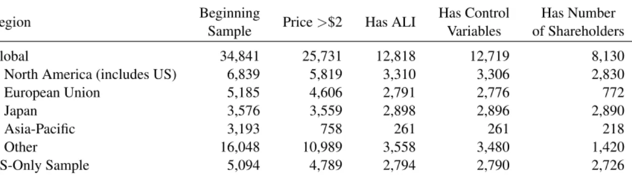
In table 1 I report the results of my sample selection process in Table 1. Panel (a) focuses on
distinct firms, and panel (b) on distinct firm-years. My initial sample comprises all publicly traded
firms for which data are available in FactSet Prices, FactSet Fundamentals, and FactSet Estimates,
beginning in 1984, the first year in which FactSet Prices data exist. From this sample I eliminate
firm-years with beginning-of-year prices under USD 2, and restrict the sample to firm-years in which
I am able to calculate an ALI1. I also eliminate from my sample any firms with missing control
variables. Finally, in my detailed cost-of-capital tests I require that the number of shareholders be
available. Most of the attrition in this step comes from EU countries, and is likely attributable to EU
countries having different reporting requirements for the number of shareholders relative to the US,
Japan, and the Asia-Pacific countries. My restrictions reduce the final global sample to 8,130 firms
1
and 88,624 firm-years, and the final US subsample (which is a strict subsample of the global sample)
to 2,726 firms and 34,879 firm-years.
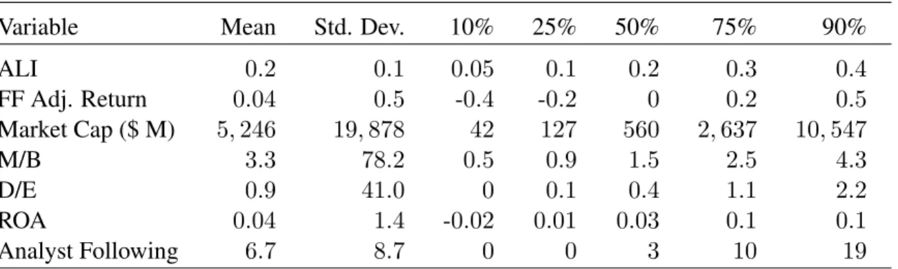
Table 2 panel (a) presents descriptive statistics on the global sample. The average market
capitalization is $5.246 B, the mean ROA is 4.4%, and the mean analyst following is 6.7 analysts.
Panel (b) shows the same statistics for the subsample of US firms. US firms tend to be larger,
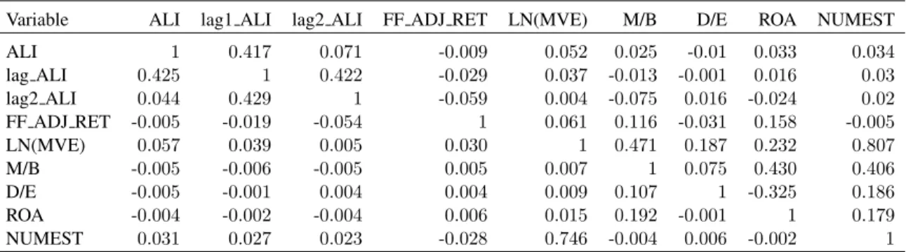
have a higher M/B ratio, and have a lower mean adjusted return. Finally, Table 3 presents Pearson
(Spearman) correlations for the variabels I use in my regression tests below (above) the diagonal.
Constructing ALI only requires a time series of past returns. This is a useful feature of the
measure, since price and return data are widely available for many firms in many countries and from
many sources. However, a fairly long time series is required to calculate ALI. Recall that calculating
ALI for yeartrequires a vector of risk factor returns for five previous years,[t−5, t−1]. Moreover, calculating the return for yeart−5itself requires an additionalv−1years prior to yeart−5, where
vis the number of eigenvectors to be calculated. Since I am extracting 4 vectors, that means that a nine-year time series (including yeart) is required to calculate the ALI in my primary tests2. The requirement that a firm in yearthave an unbroken time series of prices over the previous eight years creates a marked tilt toward larger firms, and I therefore note that am unable to assess whether the
ALI is associated with the features or behavior of very young firms.
2
CHAPTER 5
TEST DESIGN AND RESULTS
5.1
Tests of Hypothesis 1
To test H1, I regress analyst following on ALI and control variables that come from the extant
literature. My first specification examines the contemporaneous association between ALI and
NUMEST:
N U M ESTi,t=α+β1ALIi,t+
X
γCON T ROLSi,t+θF IXED EF F ECT S+i,t, (11)
whereN U M EST is the number of analysts included in the FactSet consensus estimate for the most-covered item in the FactSet Estimates Basic Annual Focus table,idenotes firms, andtdenotes years. Control variables include the firm’s market-to-book and debt-to-equity ratio, and firm size as
measured by the natural log of market cap. All variables are defined in appendix A. Year and industry
fixed effects are included, with industry fixed effects being defined at the FactSet industry level
(approximately 150 distinct industries). A positive coefficient onβ1is consistent with the hypothesis that analysts shift their coverage promptly in response to investor demand for information measured
by ALI (H1a). Separately, because analyst coverage tends to be sticky, I allow for the possibility that
analyst coverage only changes in response to sustained investor attention, which the contemporaneous
firm-year level ALI will likely do a poor job of capturing. To assess whether sustained high investor
attention measured by ALI is associated with analyst following, I also estimate a specification with
lagged values of ALI:
N U M ESTi,t =α+β1ALIi,t+β2ALIi,t−1+β3ALIi,t−2+ X
γCON T ROLSi,t
+θF IXED EF F ECT S+i,t.
In equation (12) a positive coefficient onβ2orβ3indicates that the lagged ALI was associated with analyst coverage in yeart, consistent with analysts responding slowly to investor attention measured by ALI (H1b).
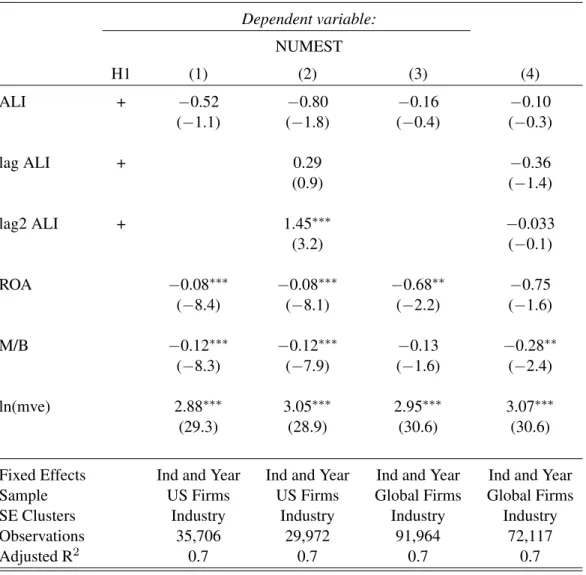
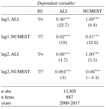
Table 4 reports the results of estimating equations (11) and (12), which test hypotheses 1a and
1b. Hypothesis 1a states that there is a positive contemporaneous association between a firm’s ALI
and its analyst following. The results in table 4, column (1) offer no support for H1a. The coefficient
on ALI is negative but insignificant, indicating that there is no contemporaneous association between
ALI and analyst coverage. The second specification (column 2), however, offers some support for
H1b. The two-year lag of ALI is associated with yeartanalyst coverage, while yeartALI is negative and marginally significant.
I consider two possible explanations for these results. The first is that analyst coverage is sticky,
so that it takes a sustained, high demand for information to induce analysts to cover a firm. The
second is that ALI is lower for firms with more revelatory prices, so the contemporaneous analyst
coverage itself may be driving the yeartALI down by increasing the information contained in the price signal. Taken together, these explanations would explain the negative (but insignificant)
contemporaneous relation between the ALI and analyst coverage and the lagged positive relation.
I repeat the analysis in columns (1) and (2) using the global sample, and present those results in
columns (3) and (4). In the global sample, neither the contemporaneous nor the lagged ALI is
associated with analyst coverage.
It may, however, be problematic to regress analyst following on ALI because of endogenous
relations between ALI and analyst coverage. Analyst coverage is likely to respond to investors’
learning incentives, and to shape them by changing the information content of prices. In addition,
investor incentives to learn about firms and analyst coverage may be in part simultaneously determined
by other factors. While conceptually one could seek to disentangle the relations between the and
analyst coverage by using appropriate instruments or exogenous shocks, the factor-based construction
of ALI makes it difficult to identify appropriate instruments. Moreover, while exogenous shocks
to realized measures of investor attention are available, they do not necessarily capture shocks in
investors’ ex-ante learning incentives. Therefore, in order to assess the inferential risks to inferences
arising from bi-directional relations between ALI and analyst coverage, I employ panel VAR models
and Bond (1998) as implemented in R by Sigmund and Ferstl (2018). Panel VAR techniques combine
elements of VAR models, which allow multiple endogenous variables to affect each other over time,
and panel data techniques that allow members of the panel to be heterogenous.
In recent years, panel VAR models have started to be used in accounting and finance in situations
where the dynamic interplay between two or more possibly endogenous variables is of interest. For
example, Desai, Rojgopal, and Yu (2016) emply a panel VAR model to examine the lead-lag relations
between short interest, analyst recommendations, and credit ratings and Margolin, Mahlendorf, and
Schaffer (2019) uses a panel VAR model to examine the bidirectional relationship between customer
satisfaction and firm performance. While panel VAR models cannot establish (econometric) causality,
they can usefully describe multi-directional associations over time and demonstrate Granger-causality
(Granger (1969)), where a change in one time series reliable produces a change in a future time
series. The basic setup of the model that I estimate is:
ALIi,t= k=n
X
k=1
γiN U M ESTi,t−k+ k=n
X
k=1
βiALIi,t−k+θi+i,t
N U M ESTi,t= k=n
X
k=1
γiN U M ESTi,t−k+ k=n
X
k=1
βiALIi,t−k+θi+i,t
(13)
where i indexes firms, t indexes years, the fixed effects are removed through a first-difference transformation, and the equations are estimated through a GMM estimator rather than OLS to avoid
Nickell bias (Nickell, 1981) as is standard in this approach1 Significant coefficients on the
non-autocrollative lags indicate Granger-causal relations between the variables, and significant positive
values for the betas in the NUMEST equation in particular would be consistent with H1b.
When I examine the time series results from the panel vector autoregression tests it is the case
that ALI has significant ability to predict future analyst coverage, and that analyst coverage has
significant ability to predict future ALI values. Table 5 presents results for estimating equation (13)
withn= 2lags. The number of lags I include in the panel vector autoregressive model is dictated by the Baysian information criterion (BIC) and the Akaike information criterion (AIC) (Andrews
and Lu, 2001; Sigmund and Ferstl 2018), and by the number of lags for which the coefficients are
1
significant. I estimate equation (13) with 1, 2, 3, and 4 lags, and find that the AIC and BIC indicate
approximately equal model fit for one and two lags with AIC values of−206and−195respectively. Model fit declines significantly with the inclusion of more than two lags2. Column 1 of Table 5
presents the results for the regression with ALI as the dependent variable, while column 2 presents
the results with NUMEST as the dependent variable. The results in column 2 indicate that analyst
following is highly persistent, with a coefficient greater than0.8on the first lag of NUMEST, and that high learning incentives predict increased future analyst following in the future. While this is
not tight evidence of a causal relation, it shows that the time series evolutions of ALI and analyst
following are consistent with H1b.
5.2
Tests of Hypothesis 2
To test H2, I regress one-year-ahead Fama-French 3-factor adjusted returns on ALI as well as a
set of control variables and fixed effects suggested by prior literature:
F F ADJ RET U RNi,t =α+β1ALIi,t+
X
γCON T ROLS
+XθF IXED EF F ECT S+i,t.
(14)
F F ADJ RET U RNi,t is the realized return for firmiin yeartless the return predicted by the
Fama-French 3-factor model. I obtain data on the Fama-French factor returns from Ken French’s
website, and I calculate firms’ loadings on the three factors as of January in yeartbased on the prior 60 months. I then subtract the predicted 3-factor return over yeartfrom the realized return overtto get the 3-factor adjusted return. The remaining controls and fixed effects are similar to the analyst
forecast regression specification (12).
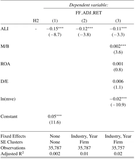
In table 6 I present the results of estimating equation (14), which tests the association between
ALI and factor-adjusted future returns. NV (2009) predicts that the learning index will be negatively
associated with factor-adjusted returns, as investors will increase the precision of information in the
market as they learn more about the firm. The results in table 6 panel (a) are broadly consistent with
that prediction for the US-only sample. The first specification in panel (a) is a simple linear regression
of one-year-ahead Fama-French 3-factor adjusted returns on ALI. The coefficient on ALI is negative
and statistically significant, as predicted. In specification 2 that adds industry and year fixed effects
and clusters standard errors by firm, the coefficient on ALI though slightly smaller in magnitude is
also negative and significant. Specification 3 keeps the same fixed-effect and clustering structure and
adds control variables, and while the coefficient on the ALI becomes slightly less negative it remains
negative and significant. The association between ALI and Fama-French adjusted future returns is
economically material as well as statistically significant. The average standard deviation of ALI
within an industry-year in my sample is .07. In the third specification, then, a one-standard-deviation
increase in ALI would imply an approximately 70 basis point lower annual adjusted return.
Panel (b) of table 6 repeats the analysis in specification (3) of panel (a) with a variety of cuts of the
global sample of firms. Column (1) includes all firms, column (2) restricts the sample to non-US firms
only, and column (3) restricts the sample to non-US developed-economy firms per Fama & French
(2012) (The US, Canada, Japan, Singapore, Hong Kong, Australia, New Zealand, Austria, Belgium,
Denmark, Finland, France, Germany, Greece, Ireland, Italy, the Netherlands, Norway, Portugal,
Spain, Sweden, Switzerland, and the UK). The estimated coefficient on ALI remains negative in
all specifications, and is significant in all but the developed economies subsample3. Although the
magnitude of the association between ALI and one-year-ahead adjusted returns weakens for countries
outside of the US, this results in table 6 panel (b) reinforce the results in panel table 6 panel (a), and
support for hypothesis 2. Overall, I regard the results in table 6 as consistent with hypothesis 2, and
with the predictions of NV (2009) regarding the learning index more broadly.
5.3
Tests of Hypothesis 3
The final prediction in NV (2009) regarding the empirical learning index is that it will exhibit an
inverted-U shaped association with home bias. The intuition behind the prediction is that in countries
whose firms have very low learning index values even domestic investors, with their information
advantage, will not find it worthwhile to learn about domestic firms. At the other extreme, in countries
whose firms have very high learning index values foreign investors will choose to learn about the
3
country’s firms despite their information disadvantage, thus reducing the level of home bias. On the
other hand, investors in countries whose firms have intermediate learning index values will find it
substantially more valuable to build on their information advantage and acquire information about
local firms, leading to a more pronounced home bias. I calculate the home bias of a fund as the
fraction of the fund’s equities held in publicly traded domestic firms minus the fund country’s share
of the global public equity market. I define the home bias of a country as the home bias of its median
fund when all funds in a country are ranked by their home bias, and the learning index of a country
as the average of the country’s firms’ ALI values. To test H3 I estimate the following regression:
HOM EBIASi,t =α+β1ALIi,t+β2ALIi,t2 +θi+i,t. (15)
The combination of a linear term and a squared term aims to assess whether the predicted quadratic
form of the association between home bias and ALI is present. The predicted association is an
inverted-U shape, viz.β1 >0andβ2 <0.
Figure 1 shows average home bias in countries when grouped into quintiles by their country-level
mean ALI. The visual evidence is consistent with hypothesis 3, with median-fund home bias being
approximately 5–7 percentage points (or about 12–17 percent) higher for countries in the 3rd ALI
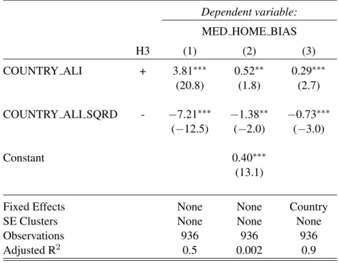
quintile than those in the 1st or 5th. In table 7 I provide more statistically rigorous evidence by
regressing median-fund home bias on the country’s annual ALI and ALI squared. Specification 1
suppresses the intercept, implying an assumption that countries with an ALI of zero would have no
home bias. Specification 2 preserves an intercept, allowing linear and quadratic ALI terms to explain
variance around it. Finally, specification 3 includes country-level fixed effects rather than a single
intercept. The results in each specification show a reliably positive linear coefficient and a reliably
negative quadratic coefficient. These results are consistent with hypothesis 3, and together with the
visual evidence in Figure 1, provide empirical evidence that ALI is captures the theoretical construct
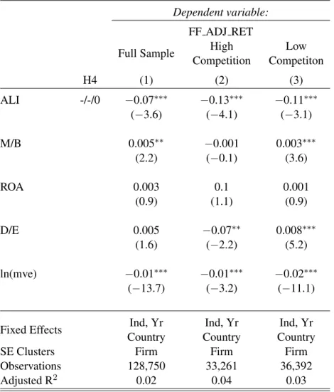
5.4
Tests of Hypotheses 4 and 5
To test H4, H5a and H5b, I follow Armstrong, Core, Taylor, and Verrecchia (2011) and use the
number of shareholders in a firm as a proxy for the competitiveness of the market for the firm’s equity,
and the firm’s one-year-ahead factor-adjusted returns as a proxy for its cost of equity. LLV (2012)
present a theory model in which information asymmetry should not affect a firm’s cost of capital
in situations of perfect competition. Using the number of shareholders to measure equity-market
competitiveness and factor-adjusted one-year-ahead returns to measure a firm’s cost of capital, ACTV
(2011) find empirical evidence consistent with this. ACTV (2011) construct hedge portfolios long in
firms with high information asymmetry and short in firms with low information asymmetry. These
hedge portfolios are then grouped by the competitiveness of the equity markets of the firms in the
extreme information asymmetry quintiles. After controlling for the market, high-minus-low and
small-minus-big factors, the hedge portfolios for firms with less-competitive equity markets (i.e.
few shareholders) yield positive returns, while the hedge portfolios for firms with more-competitive
equity markets (i.e. many shareholders) yield no abnormal returns. While the number of shareholders
in a firm is an imperfect measure of the competitiveness of its equity market, it is readily available
for US firms and — through FactSet — for a large number of international firms as well.
I test H4 by estimating equation (11) using only firms in the top two quintiles of NUM SHRHLDRS,
the number of distinct shareholders in a firm. My assumption is that firms in the top two quintiles
of the number of shareholders will not be affected by changes that a high ALI might induce in
information asymmetry, with the result that any effect on future returns is likely to be attributable
to the information precision channel of LLV (2012). I then separately estimate equation (11) using
only firms in the bottom two quintiles of NUM SHRHLDRS. The theory in LLV (2012) does not
allow me to make unambiguous predictions as to the sign of the association between ALI and future
returns in this sample. As the firms are all in less-competitive equity markets, any effect which
ALI has on information asymmetry should be apparent in future returns, along with any effect the
ALI has on information precision. Since increased attention could increase or decrease information
asymmetry, but should only increase information precision, I expect the most likely outcome to be a
more positive (i.e. less negative) association between ALI and future returns than the association
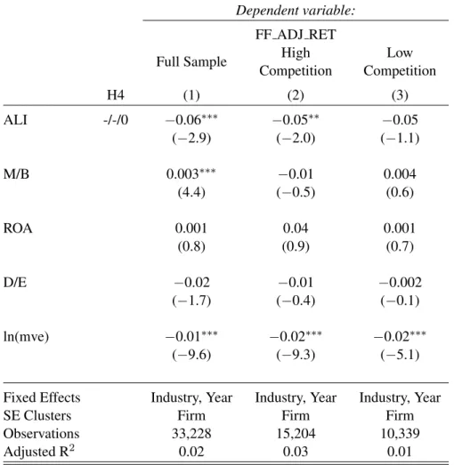
Table 8 resports the results of estimating equation (11) on the sample cuts just described.
Specification 1 in table 8 panel (a) repeats specification 3 in table 6, but with ALI re-computed within
the US sample. The results are inferentially similar. Specification 2 then restricts the sample to
firms with NUM SHRHLDRS in the top two quintiles of the US sample, and the coefficient on ALI
remains negative and significant. The interpretation of the latter result is that, in a setting where
information asymmetry is expected to have no (or little) effect, the association between ALI and
a firm’s cost of equity remains negative, which is consistent with investors seeking out additional
information about high-ALI firms and thereby improving the precision of the market’s expectation of
those firms’ performance. As such, the test aims to isolate the information-precision channel through
which ALI might affect future returns.
In Specification 3 I adjust the sample criterion in specification 2 and instead restrict the sample to
firms with NUM SHRHLDRS in the bottom two quintiles of the US sample. In this setting I expect
both information asymmetry and the quality of the market’s information about a firm to influence
future returns. The estimated coefficient on ALI in remains negative but loses significance, which is
consistent with an improvement in the quality of information about a firm being offset by increases
in information asymmetry due to increases in investors’ demand for information about a firm. This
increase in information asymmetry is consistent with a setting where all investors have a desire to
acquire information about a firm, but only some investors are able to do so.
Taken together, I posit that the results in table 8 panel (a) support hypothesis 4. ALI is negatively
associated with the future factor-adjusted returns, but only significantly for firms whose equity
is widely held. This indicates that among firms whose equity markets are competitive, ALI is
clearly associated with lower future returns, whereas the situation is ambiguous for firms having
less-competitive equity markets. I turn to those firms in my test of hypothesis 5 below.
I test H5a by re-estimating equation (11) using firms that are in the bottom two quintiles of
market competition and in the top quartile of analyst coverage. I use analyst coverage to measure
the quality of a firm’s information environment. In testing H5a, I seek to focus on firms where,
despite an imperfectly competitive equity market, it is feasible for investors to satisfy an increased
demand they may have for information. I assume that analyst coverage is a reasonable proxy for
that construct, also but re-estimate equation (11) using the bottom quartile of media coverage in