Topics in Basis Reduction and Integer Programming
Mustafa Kemal Tural
A dissertation submitted to the faculty of the University of North Carolina at Chapel Hill in partial fulfillment of the requirements for the degree of Doctor of Philosophy in the Department of Statistics and Operations Research.
Chapel Hill 2009
Approved by:
Shu Lu
G´abor Pataki
Scott Provan
David Rubin
Abstract
MUSTAFA KEMAL TURAL: Topics in Basis Reduction and Integer Programming (Under the direction of G´abor Pataki)
A basis reduction algorithm computes a reduced basis of a lattice consisting of short and nearly orthogonal vectors. The best known basis reduction method is due to Lenstra, Lenstra and Lov´asz (LLL): their algorithm has been extensively used in cryptography, experimental mathematics and integer programming. Lenstra used the LLL basis reduction algorithm to show that the integer programming problem can be solved in polynomial time when the number of variables is fixed.
In this thesis, we study some topics in basis reduction and integer programming. We make the following contributions.
We unify the fundamental inequalities in an LLL reduced basis, which express the shortness and near orthogonality of the basis.
We analyze two recent integer programming reformulation techniques which also rely on basis re-duction. The reformulation methods are easy to describe. They are also successful in practice in solving several classes of hard integer programs.
First, we analyze the reformulation techniques on bounded knapsack problems. The only analyses so far are for knapsack problems with a constraint vector having a certain decomposable structure. Here we do not assume any a priori structure on the constraint vector.
We then analyze the reformulation techniques on bounded integer programs. We show that if the coefficients of the constraint matrix are drawn from a sufficiently large interval, then branch and bound creates at most one node at each level if applied to the reformulated instances.
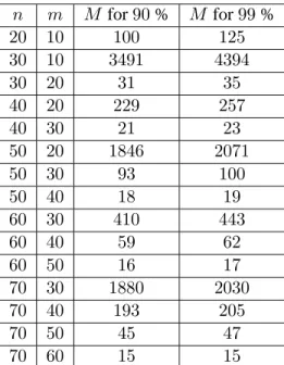
On the practical side, we give some numerical values as to how large the numbers should be to make sure that for90and99percent of the reformulated instances, the number of subproblems that need to be enumerated by branch and bound is at most one at each level. These values turned out to be surprisingly small when the problem size is moderate.
Acknowledgements
I would never have been able to finish my dissertation without the guidance of my committee mem-bers, help from friends and support from my family and wife.
First of all, I would like to express my deepest gratitude to my advisor Dr. G´abor Pataki for his invaluable guidance, advice and inspiration during my graduate study. I would like to thank Dr. David Rubin for carefully going through my dissertation and suggesting corrections. I would also like to thank my other dissertation committee members Dr. Shu Lu, Dr. Scott Provan and Dr. Jon Tolle.
I want to thank Dr. Serhan Ziya for his support throughout my graduate study. I also want to thank Dr. Edcard Carlstein who has been a remarkable teaching advisor. Dr. Edcard Carlstein was always there to listen and to give advice.
I am deeply indebted to my parents, Makbule Tural and Veysi Tural. Their love and support provided me the energy to attain my study.
Table of Contents
List of Tables . . . vii
List of Figures . . . viii
1 Introduction . . . 1
2 Notation, Definitions and Basic Results . . . 5
2.1 Basics . . . 5
2.2 Lattices and Basis Reduction . . . 6
2.2.1 LLL Reduced Bases . . . 10
2.2.2 KZ Reduced Bases . . . 11
2.2.3 Hermite Normal Form . . . 12
2.2.4 Null, Orthogonal, Dual and Complete Lattices . . . 13
2.2.5 RKZ Reduced Bases . . . 15
2.3 Integer Programming and Branch and Bound . . . 16
2.3.1 The Algorithms of Lenstra and Kannan for Integer Programming. . . 18
2.3.2 Two Integer Programming Reformulation Techniques . . . 22
3 Unifying LLL Inequalities . . . 25
3.1 Generalizations of the Fundamental Inequalities in LLL Reduced Bases . . . 25
3.2 Proofs of Theorem 1 and Theorem 2 . . . 28
3.3 Discussion . . . 31
4 Branching on a Near Parallel Integral Vector in a Knapsack Problem . . . 32
4.1 Reformulations of the Knapsack Problem . . . 32
4.3 Near Parallel Vectors: Intuition and Proofs of Theorems 4 and 5 . . . 38
4.4 Branching on a Near Parallel Vector: Proof of Theorem 6 . . . 42
4.5 Successive Approximation . . . 44
4.6 Discussion . . . 46
5 Branching Proofs of Infeasibility in Low Density Subset Sum Problems . . . 48
5.1 Introduction . . . 48
5.2 Literature Review . . . 48
5.3 Main Results . . . 50
5.4 Proofs . . . 52
5.5 Discussion . . . 56
6 Basis Reduction and the Complexity of Branch and Bound . . . 58
6.1 Introduction and Main Results . . . 58
6.2 Computational Study . . . 66
6.3 Further Notation and Proofs . . . 67
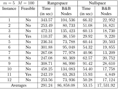
6.4 Detailed Computational Results . . . 73
7 On the Hardness of Subset Sum Problems by Ordinary Branch and Bound . . . 77
7.1 Introduction and Main Result . . . 77
7.2 Summary of the Solvability of Subset Sum Problems by Branch and Bound . . . 80
8 Summary and Future Research . . . 81
List of Tables
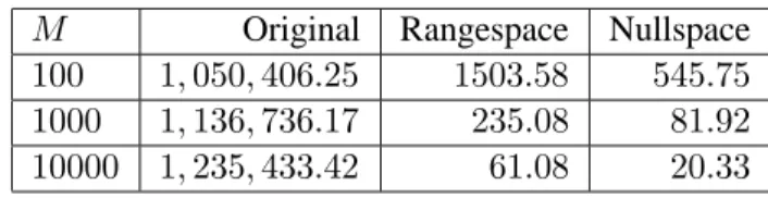
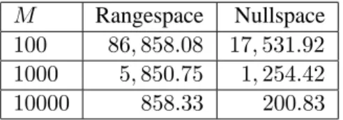
6.1 Values ofMto make sure that the RKZ-nullspace reformulation solve at the root node 64
6.2 Average number of B&B nodes to solve4-by-30marketshare problems . . . 66
6.3 Average number of B&B nodes to solve5-by-40marketshare problems . . . 67
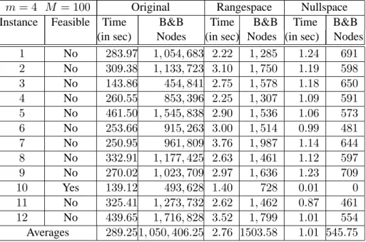
6.4 Results for the randomly generated4by30marketshare instances whenM = 100. . . 73
6.5 Results for the randomly generated4by30marketshare instances whenM = 1000 . . 74
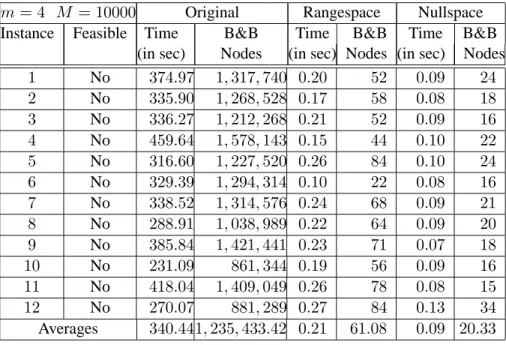
6.6 Results for the randomly generated4by30marketshare instances whenM = 10000 . 74
6.7 Results for the randomly generated5by40marketshare instances whenM = 100. . . 75
6.8 Results for the randomly generated5by40marketshare instances whenM = 1000 . . 75
List of Figures
2.1 A Lattice inR2. . . 8
2.2 A Lattice with no Orthogonal Basis. . . 9
2.3 LP Relaxations of the Problem in Example 4 and its Rangespace Reformulation . . . . 23
CHAPTER 1
Introduction
Algorithms based on geometry of numbers have been an essential part of the integer programming (IP) landscape starting with the work of H. W. Lenstra [36]. Typically, these algorithms reduce an IP feasibility problem to a provably small number of smaller dimensional ones and have strong theoretical properties. For instance, the algorithms of [27,36,39] have polynomial running time in fixed dimension; the algorithm of [14] has linear running time in dimension two. One essential tool in creating the subproblems is a “thin” branching direction, i.e., an integral (row-)vectorcwith the difference between the maximum and the minimum of cx over the underlying polyhedron being provably small. Basis reduction in lattices – in the Lenstra, Lenstra and Lov´asz (LLL) [35], or Korkine and Zolotarev (KZ) [27,30] sense – is usually a key ingredient in the search for a thin direction. For implementations and computational results, we refer to [10,18,41].
A simple and experimentally very successful reformulation technique for integer programming was proposed by Aardal, Hurkens and A. K. Lenstra in [2] for equality constrained IP problems; see also [1]. For several classes of hard equality constrained integer programming problems – e.g., [11] – the reformulation turned out to be much easier to solve by commercial solvers than the original problem.
In [31] an experimentally just as effective reformulation method was introduced, which leaves the number of the variables the same and is applicable to both inequality or equality constrained problems. These reformulation methods are very easy to describe (as opposed to say Lenstra’s and Kannan’s methods), but seem difficult to analyze. The only analyses are for knapsack problems, with the weight vector having a given “decomposable” structure. See [3,31].
notions of reducedness. In this thesis, we will use LLL, KZ, and RKZ reduced bases. An LLL reduced basis of a lattice can be computed in polynomial time for rational lattices. The first vector of an LLL reduced basis of a latticeLis an approximation of a nonzero shortest vector inL. In an LLL reduced basis, as shown in [35], the norm of the first vector is bounded by a function of the norm of a nonzero shortest vector of Land also by a function of the determinant ofL. The product of the norms of the basis vectors is also bounded by a function of the determinant ofL. We call these three inequalities “the fundamental inequalities of an LLL reduced basis”. KZ [27,30] and RKZ [32] reduced bases have stronger reducedness properties, but are only computable in polynomial time when the dimension n of the lattice is fixed. Section2.2provides some details about basis reduction and different notions of reducedness.
This thesis studies some topics in geometry of numbers and integer programming. It makes the following contributions:
(1) It generalizes the fundamental inequalities for an LLL reduced basis.
(2) It provides an analysis of the IP reformulation techniques for knapsack problems without assum-ing any a priori structure on the constraint vector.
(3) It resolves the question of the solvability of an overwhelming majority of the subset sum (fea-sibility) problems (all but a vanishing proportion of the problems as n increases) in polynomial time using the method of branch and bound. We will assume that the coefficients of the subset sum problems are chosen from a sufficiently large interval of integers. In more detail, we have the following results. We show that an overwhelming majority of the subset sum problems are hard for ordinary branch and bound. On the other hand, an overwhelming majority of the subset sum problems are easy for generalized branch and bound. Moreover, if we reformulate the subset sum problem using the rangespace [31] or the nullspace [2] reformulation, then an overwhelming majority of the reformulated problems become easy for ordinary branch and bound. Here the word “easy” means the problem is solved in polynomial time and at most one branch and bound node is created at each level of the branch and bound tree in the process of solving it. A “hard” problem, however, can be solved only by creating an exponential number of nodes.
suffi-ciently large interval, then for almost all such instances the number of subproblems that need to be enumerated by branch and bound is at most one at each level of the branch and bound tree (when applied to reformulated instances).
(5) On the practical side, it provides numerical values ofMwhich ensure that at least90and99 per-cent of the reformulated (binary) instances (with coefficients chosen from{1, . . . , M}) solve in at mostnsubproblems. These numbers are surprisingly small for moderate-size binary problems.
(6) It computationally confirms the somewhat counter-intuitive finding: the reformulations of random integer programs tend to get easier, as the coefficients become larger.
The rest of the thesis is organized as follows. In Chapter2, we give notation, definitions and basic results that will be used throughout the proposal. Here, we introduce a modified version of Lenstra’s algorithm which potentially uses a smaller number of rounding and basis reduction steps.
In Chapter3, we unify and generalize the fundamental inequalities for an LLL reduced basis. In Chapter4, we analyze two integer programming reformulations of the knapsack problem, namely the rangespace and the nullspace reformulations. We first show that in a knapsack problem, branching on an integral vector which is “near parallel” to the constraint vector creates a small number of branch and bound nodes. A transference result proves an upper bound on the integer width along the last variable in the reformulated problems. This upper bound becomes 1when the density is sufficiently small, i.e., when the Euclidean norm of the constraint vector is sufficiently large.
In Chapter5, we show that for a low density subset sum problem, there is a polynomial time com-putable certificate of infeasibility for almost all integer right hand sidesβ. Using a transference result, we prove that for almost all right hand sides, the integer width along the last variable in the rangespace reformulation of a low density subset sum problem is zero.
CHAPTER 2
Notation, Definitions and Basic Results
2.1
Basics
Leth., .ibe the Euclidean scalar product onRm, i.e., for anyx, y∈Rm
hx, yi= m X
i=1 xiyi,
wherexiandyiare theith components ofxandy, respectively. We usek.kork.k2 for the Euclidean norm, i.e. for anyx∈Rm
kxk=kxk2=phx, xi.
Two other norms will be important for our purposes: theℓ1 norm and theℓ∞norm
kxk1= m X
i=1 |xi|
kxk∞= max i |xi|.
When we want to talk about theℓ1orℓ∞norms of a vector, we explicitly say so. When we just say “norm ofx”, we mean the Euclidean norm ofx.
It is known that for allx∈Rm, the following relations hold:
kxk ≤ kxk1 ≤√mkxk, (2.1.1)
kxk∞ ≤ kxk1 ≤mkxk∞. (2.1.3)
For anyx, y∈Rm, we have the Cauchy-Schwarz Inequality:
|hx, yi| ≤ kxkkyk. (2.1.4)
Equality holds if and onlyxandyare linearly dependent.
For a matrix B, Bij is the entry at the intersection of ith row andjth column ofB. We let BT
denote the transpose ofB. For an invertible matrixB,B−1 denotes the inverse ofB andB-T denotes
the transpose of the inverse ofB.
For an m-by-m matrix B = [b1, . . . , bm], det(B) represents the determinant ofB. B is called nonsingular ifdet(B)6= 0, otherwise it is singular. We have Hadamard’s Inequality
|det(B)| ≤ m Y
i=1
kbik. (2.1.5)
Equality holds if and only if either both sides are zero or the vectorsb1, . . . , bmare orthogonal.
For matrices (and vectors) AandB with appropriate dimensions, we write(A;B)for
A
B
; and we write(A, B)for(A B).
2.2
Lattices and Basis Reduction
A lattice inRmis a set of the form
L = L(B) = {Bx|x∈Zn}, (2.2.6)
whereB is a real matrix withmrows and nindependent columns, called a basis of L. A lattice has infinitely many different bases whenn≥2. Any basisBof a latticeLhas the same number of columns, called the dimension ofL. A square, integral matrixU is unimodular ifdet(U) =±1. It is well known thatB1andB2are bases of the same lattice if and only ifB2 =B1U for some unimodularU.
An elementary column operation performed on a matrixB is either
(2) multiplying a column by−1, or
(3) adding an integral multiple of a column to another column.
Multiplying a matrix B from the right by a unimodular U is equivalent to performing a sequence of elementary column operations onB.
The determinant ofL is
detL = (det(BTB))1/2, (2.2.7)
whereB = [b1, . . . , bn]is a basis ofL; it is easy to see that detLis well-defined. From Hadamard’s Inequality, it follows that
detL ≤ n Y
i=1 kbik.
The determinant of a lattice is then-dimensional volume of the paralelepiped defined by any basis of the lattice (see Figure2.1).
A latticeLinRmis full dimensional if dimension ofLis equal tom. EquivalentlyL⊆Rmis full dimensional if and only if the smallest subspace ofRmcontainingLisRm.
Example 1. LetΛ =L(B1)where
B1= 3 2 2 2 .
LatticeΛconsists of all integral vectorsx∈Z2such thatx2is even. The green area defined by the
columns ofB1is equal todet Λwhich is2.
LatticeΛis also generated by the columns of
B2= 1 5 0 2 ,
sinceB2 =B1U, where
U =
1 3
−1 −2
is a unimodular matrix. The pink area defined by the columns ofB2is also equal to2.
Figure 2.1: A Lattice inR2.
Example 2. LetΓ =L(B2)where
B2=
1 3
3 2
.
The lattice Γ does not have any orthogonal basis. Note that both Λ and Γ are full dimensional
lattices.
Suppose thatBhasnindependent columns
B = [b1, . . . , bn], (2.2.8)
andb∗
1, . . . , b∗nform the Gram-Schmidt orthogonalization ofb1, . . . , bn, that isb1 =b∗1, and
bi =b∗i + i−1 X
j=1
µijb∗j with µij = bTi b ∗ j/kb
∗
Figure 2.2: A Lattice with no Orthogonal Basis.
In terms of the Gram-Schmidt vectors,
detL(B) = n Y
j=1
kb∗jk. (2.2.10)
Each latticeLcontains a nonzero shortest vector. Letλ1(L)denote the norm of a nonzero shortest vector inL. Minkowski’s convex body theorem implies that
λ1(L)≤√n(detL)1/n, (2.2.11)
wherenis the dimension ofL. See for instance [27].
Turning back to our previous examples, we haveλ1(Λ) = 1andλ1(Γ) = √
5.
2.2.1 LLL Reduced Bases
The LLL basis reduction algorithm [35] was introduced in 1982 by Lenstra, Lenstra and Lov´asz; and has since been used in numerous applications in computational mathematics and computer science starting with factoring polynomials with rational coefficients and solving the integer linear programming problem in polynomial time in fixed dimensions. It computes a reduced basis of a lattice in polynomial time (for rational lattices). For simplicity, we use Schrijver’s definition from [47].
We callB= [b1, . . . , bn]an LLL reduced basis of L(B), if
|µij| ≤ 1/2 (i= 2, . . . , n;j= 1, . . . , i−1), and (2.2.12) kb∗
ik2 ≤ 2kb∗i+1k2 (i= 1, . . . , n−1). (2.2.13)
From (2.2.13) it immediately follows that
kb∗
ik2 ≤ 2j−ikb∗jk2 (1≤i≤j ≤n). (2.2.14)
As shown by Lenstra, Lenstra and Lov´asz, in an LLL reduced basis B = [b1, . . . , bn]of a lattice L=L(B), the norm of the first vector is bounded by a function of the norm of a nonzero shortest vector
ofLand also by a function of the determinant ofL, namely
kb1k ≤ 2(n−1)/4(detL)1/n, (2.2.15)
kb1k ≤ 2(n−1)/2 kdk for any d∈L\ {0}. (2.2.16)
For an LLL-reduced basisB = [b1, . . . , bn]of a latticeL, they also show that
kb1k · · · kbnk ≤ 2n(n−1)/4detL. (2.2.17)
2.2.2 KZ Reduced Bases
Korkine-Zolotarev (KZ) reduced bases, which were described in [30] by Korkine and Zolotarev, and by Kannan in [27], have stronger reducedness properties than LLL reduced bases. For instance, the first vector in a KZ reduced basis is a shortest vector of the lattice. However, KZ reduced bases are computable in polynomial time only whennis fixed.
Given anm-by-nmatrixD= [d1, . . . , dn]with rankr,span(D)(orspan{d1, . . . , dn}) is defined as
span(D) ={Dx|x∈Rn}. (2.2.18)
span(D)is anr-dimensional subspace ofRm.
LetL = L(B)whereB = [b1, . . . , bn]with n independent columns and forj < iletbi(j)be the projection ofbiorthogonal tospan{b1, b2, . . . , bj}. Note thatbi(i−1) =b∗i. Let
L(j) =L([bj+1(j), . . . , bn(j)])
be the projection ofLorthogonal to span{b1, b2, . . . , bj}. For convenience we definebi(0) = bi and L(0) =L.
We say that a basisB= [b1, . . . , bn]is a KZ reduced basis ofL(B)if
(1) |µij| ≤1/2 (i= 2, . . . , n;j= 1, . . . , i−1), and
(2) bi(i−1)is a shortest nonzero vector ofL(i−1) (i= 1, . . . , n).
Note that ifB= [b1, . . . , bn]is a KZ reduced basis, thenb1is a shortest nonzero vector inL(B). For a KZ reduced basisB = [b1, . . . , bn]of a latticeL=L(B), from the definition of a KZ reduced basis and (2.2.11), it follows that
kb∗jk≤pn−j+ 1 n Y
i=j
kb∗ik1/(n−j+1), (2.2.19)
for anyj∈ {1, . . . , n}. In particular, forj = 1(2.2.19) becomes
It was also shown [32] that
kb∗ik≥ λ1(L)
i(1+logi)/2 (2.2.21)
holds fori= 1, . . . , n.
Schnorr in [44] proposed several hierarchies of bases between LLL and KZ reduced ones: the semi block2kbases among them are polynomial time computable whenkis fixed; and both the “quality” of the basis, and the complexity of the reduction algorithm increases withk.
2.2.3 Hermite Normal Form
An integralm-by-nmatrix with full row rank (i.e., with rankm) is in Hermite Normal Form (HNF) if it has the form[B,0], whereB is a lower triangular, nonnegative matrix with each diagonal entry being the unique maximum in its row, and0is the matrix of all zeroes with appropriate size. Note that B is a nonsingular matrix. Any integral matrix Awith full row rank can be brought into HNF by a series of elementary column operations [23] and this can be done in polynomial time as shown in [28]. In other words, there exists a polynomial time computable unimodular matrixU such thatAU = [B,0] is in HNF. It is known that the HNF ofAis unique and we writeHNF(A) = [B,0].
Letgcd(A)be the greatest common divisor of them-by-msubdeterminants ofA. Note thatgcd(A) is invariant under elementary column operations. Therefore, we have that
gcd(A) = m Y
i=1
Bii, (2.2.22)
whereHNF(A) = [B,0].
Example 3. Let
A =
1 2 7
3 4 1
The 2-by-2 subdeterminants ofAare−2,−20, and−26. Thereforegcd(A) = 2. We have
HNF(A) =A
−1 2 13
1 −1 −10
0 0 1
=
1 0 0
1 2 0
.
2.2.4 Null, Orthogonal, Dual and Complete Lattices
For an integralmbynmatrixA,m≤n, the null lattice ofAis denoted byN(A)and is defined as
N(A) ={x∈Zn|Ax= 0}. (2.2.23)
For an integral latticeL, its orthogonal lattice is defined as
L⊥ = {y∈Zn|yTx= 0∀x∈L}.
Note thatN(A) is the same asL(AT)⊥. For a latticeL, the dual latticeL∗is
L∗ =
{y∈spanL| hx, yi ∈Zfor allx∈L}, (2.2.24)
wherespanLisspan(B)whereB is a basis ofL. It is known thatdet(L∗) = (det(L))−1.
LetB= [b1, . . . , bn]be a basis of the latticeL. It is easy to see thatD= [d1, . . . , dn] =B(BTB)−1 is a basis ofL∗. We callB∗ = [d
n, . . . , d1]the dual basis (or the reciprocal basis) of B(note that the columns of D are reordered). One can check that B is the dual basis of B∗ as well. If L is full dimensional, then ordering the columns ofB-Tfrom highest index to smallest gives the dual basis ofB.
LetB∗
be the dual basis ofB. And letb∗∗
1 , . . . , b∗∗n andb#1, . . . , b#n be the Gram-Schmidt orthogo-nalizations of columns ofB∗andB, respectively. Then, it is easy to check that
A latticeL⊆Znis called complete, if
L = (span L) ∩ Zn.
Each basisV of a complete latticeLcan be completed to a unimodular matrix, i.e., there exists a matrix W such that[V, W]is unimodular. Another useful characterization of complete lattices is thatL(V)is complete if and only ifHNF(VT) = [I,0]. For a proof see [43].
If a ∈ Zn, L(aT) is complete if and only if gcd(a
1, a2, . . . , an) = 1 where gcd is the greatest common divisor. The following result relates the determinants of N(A) and L(AT) where A is an
integral matrix.
Proposition 1. LetAbe an integral full row rankm-by-nmatrix. Then
detN(A) = detL(AT)/gcd(A). (2.2.26)
Proof of Proposition 1 LetV be a basis forspan(AT)∩Zn andL(V) = span(AT)∩Zn, which is an m dimensional complete lattice. We have thatAT = V M for an invertible matrix M. Therefore
M-TA=VT. SinceL(V)is complete,HNF(VT) = [I,0], which implies thatHNF(M-TA) = [I,0]as
well. Since gcd is invariant under elementary column operations,gcd(M-TA) = 1 = det(M-T) gcd(A).
This implies thatdet(M) = gcd(A). Now, we can writedetL(AT) =
det((V M)T(V M))1/2= det(M) detL(V). To finish the proof,
we need to show thatdetL(V) = detN(A).
Since L(V) is complete, V can be completed to a unimodular matrix, say U, i.e., there exists a matrixW such thatU = [V, W]is unimodular. Let U−1 = [Y;Z], where the dimensions ofY and Z are the same as the dimensions of VT and WT, respectively. The rows of Z are a basis of N(A)
and the projections of the columns ofYT orthogonal tospan(ZT)are a basis ofL(V)∗. Furthermore det(U−1) = (detL(V)∗)(detN(A)) = 1, which implies thatdetL(V)∗ = 1/(detN(A))and there-foredetL(V) = detN(A)completing the proof.
The following corollary of Proposition1, has been used in some cryptographic applications. See for instance [43].
The following lemma summarizes some basic results in lattice theory that we will use later on; for a complete proof, see for instance [40].
Lemma 1. For anmbynintegral matrixAwith independent rows andL=L(AT), the following are
equivalent
(1) Lis complete.
(2) Thegcdof the determinants of thembymsubmatrices ofAis1.
(3) HNF(A) = [I,0].
(4) There exists a matrixV such that[V;A]is unimodular.
(5) detL⊥= detL.
(6) There is a unimodular matrixZ such that
ZAT =
Im
0(n−m)×m
.
Furthermore, ifZis as in part (6), then the lastn−mrows ofZare a basis ofL⊥
.
2.2.5 RKZ Reduced Bases
Hermite’s constantCi is defined as
Ci=supn(λ1(L))2/(detL)2/i |Lis a lattice of rank i o
. (2.2.27)
Its values are known exactly only fori≤8andi= 24. It is known that [40]
Ci≤1 +i/4. (2.2.28)
Sharper asymptotic bounds are known. In our analysis, for simplicity we will use2.2.28, and for small values ofithe Blichfeldt’s upper bound [7]:
Ci ≤ 2 πΓ
i+ 4
2 2/i
whereΓ(.)is the gamma function.
A reciprocal Korkhine-Zolotarev (RKZ) basis is the dual (reciprocal) basis of a KZ reduced basis. LetB = [b1, . . . , bn]be an RKZ reduced basis ofLand let[b∗1, . . . , b∗n]be the Gram-Schmidt orthogo-nalization of its columns. It can be shown that the Gram-Schmidt vectors of an RKZ reduced basis of a lattice are not too short. Combining 2.2.20and 2.2.25we get a lower bound on the norm of the last Gram-Schmidt vector in terms of the determinant of the lattice:
kb∗nk≥ (detL) 1/n √
n . (2.2.30)
It was shown in [32] that
kb∗ ik≥
λ1(L) Ci
(2.2.31)
holds fori= 1, . . . , n.
2.3
Integer Programming and Branch and Bound
Given a polyhedronQ, an integer programming (IP) feasibility problem is the problem of finding an integral vector inQ. In this thesis, we only consider feasibility problems. To solve an IP optimization problem, one needs to solve a sequence of feasibility problems using binary search.
Branch and bound, which we will abbreviate as B&B, was first studied by Land and Doig in [34] and is a classical method for IP feasibility (and optimization, more generally). It starts withQas the sole subproblem. In a general step, one chooses a subproblemQ′, an integral vectorc, and creates new subproblems Q′
∩ {x|cx=γ}, whereγ ranges over all possible integer values thatcx can take. This is repeated until all subproblems are found to be empty, or an integral point is found in one of them. Usually the vectorscare chosen to be the standard unit vectorsei (i.e., we branch on the variablexi). In this case, at each level of the B&B tree, one variable is fixed. This is called ordinary B&B. In a
generalized B&B algorithm, the vectorscare allowed to be any integral vectors.
For a polyhedronQand an integral vectorc, the width and the integer width ofQalongcare
The integer width is the number of nodes generated by branch and bound when branching on the hyper-planecx; in particular,iwidth(ei, Q)is the number of nodes generated when branching onxi. It is easy to show that
iwidth(c, Q)≤ ⌊width(c, Q)⌋+ 1. (2.3.32)
If the integer width along any integral vector is zero, thenQhas no integral points. Given an integer program labeled by(P), andc an integral vector, we also writewidth(c,(P)),andiwidth(c,(P))for the width and the integer width of the LP relaxation of(P)alongc,respectively. Here, the LP relaxation of(P)is the underlying polyhedron describing the problem(P).
Given a lattice L with basis B = [b1, . . . , bn]and a polyhedron Q, the problem of determining whetherQcontains a lattice point ofLis a generalization of the IP feasibility problem. Letb∗
1, . . . , b∗n be the Gram-Schmidt orthogonalization ofb1, . . . , bn. A lattice pointx∈L∩Qis of the form
x= n X
j=1
λjbj, (2.3.33)
whereλj are integers. Assume thatQis contained in a sphere of radiusr. Then λn can take at most (2r/kb∗
nk) + 1different integer values. Similarly, having fixedλi+1, . . . , λn;λi can take at most
2r/kb∗ik+1 (2.3.34)
different integer values. Note that here the vectorsbi do not need to be integral vectors! This enumer-ation process is similar to branch and bound. In this enumerenumer-ation process, the total number of nodes created on the level ofbi(i.e., on the (n−i+ 1)st level) is at most
n Y
j=i
2r/kb∗ jk+1
. (2.3.35)
The algorithm is repeated for each subproblem created until an integral point is found in any of the subproblems, which implies the integer feasibility ofQ, or all the subproblems become the empty set, in which case the problem is integer infeasible. The upper bound on the number of B&B nodes created per level was later improved toO(2n)[5,38].
Kannan [27] introduced a variant of Lenstra’s algorithm which uses the KZ basis reduction algorithm instead. He showed that at the ith (1 ≤ i ≤ n) level of the branch and bound tree, there are at most (2n)5i/2 nodes (where the value of i is determined by the algorithm), which implies a polynomial number of nodesO(n5/2)per level (O(n5/2)is not an upper bound on the number of nodes created for each subproblem at each level!). Note that his basis reduction algorithm does not run in polynomial time for varyingn, but runs in polynomial time only whennis fixed.
In Section2.3.1, we will briefly describe the algorithms of Lenstra and Kannan. In Section2.3.2we will introduce two experimentally very successful reformulation techniques for IP feasibility problem, namely the rangespace reformulation introduced in [31] for general IP feasibility problems and the nullspace reformulation introduced by Aardal, Hurkens and A. K. Lenstra in [2] for equality constrained IP feasibility problems; see also [1].
2.3.1 The Algorithms of Lenstra and Kannan for Integer Programming
In this section, we will briefly describe Lenstra’s (a modified version) and Kannan’s algorithms for integer programming. This exposition is mainly based on Kannan’s survey on Algorithmic Geometry of Numbers [26].
Given an IP feasibility problem described by the polyhedron Q, these algorithms find an integral point in Qif there is any or prove thatQdoes not contain any integral point. Both algorithms run in polynomial time for fixedn.
We start with making Qa full dimensional polytope inRn if it is not already; for the details see [36]. Lov´asz in [38] developed an algorithm to transform a polytope into a “rounded” one. He showed that there exists an invertible linear transformationφsuch thatS1 ⊆P ⊆S2for two concentric spheres S1andS2whereP =φQandr2/r1 ≤(n+ 1)√nwithribeing the radius ofSi.
reduced). Letφ−1B = [φ−1b1, . . . , φ−1bn]and letD= φ−1B -T
= [d1, . . . , dn]. Bothφ−1BandD are bases ofZn(i.e., they are unimodular), sinceDis a basis of the dual lattice ofL(φ−1B) =Zn.
Letjbe the index such thatkb∗
jk≥kb∗ikfori∈ {1, . . . , n}. It is easy to show that if
r1 ≥√nkb∗jk/2, (2.3.36)
thenP contains a point ofL, sayℓwhich means thatφ−1ℓis an integral point inQ.
We modify Lenstra’s algorithm, using ideas from [26]. Below are the main steps of both of the algorithms. We assume that we start with a polytopeQ.
Algorithms
(1) Start with a polytopeQ.
(2) Make it full dimensional and letnbe the dimension of the full dimensional polytopeQ.
(3) RoundQ: find an invertible linear transformation φsuch thatP = φQis rounded. (Findr1and r2as well).
(4) Find a reduced basis B = [b1, . . . , bn] ofL = φZn and let b∗1, . . . , b∗n be the Gram-Schmidt orthogonalization ofb1, . . . , bn.
(5) Letjbe index such thatkb∗
jk≥kb∗ikfor alli∈ {1, . . . , n}.
(6) Ifr1 ≥√nkb∗jk/2, thenP contains a lattice point ofL. STOP,Qis integer feasible.
(7) Otherwise, using the basisD = [d1, . . . , dn]ofZn, apply backward B&B for n−j+ 1 levels (i.e., branch ondnx, . . . , djxin the original space in this order). Then for each nonempty sub-problem created if its dimension is0(i.e., if its a single integer point), STOP,Qis integer feasible; otherwise go to step1.
(8) If the algorithm never stops and all subproblems become the empty set, thenQis integer infeasi-ble.
Any integer point y ∈ Q∩Znis of the formPn
j=1 λj(φ−1bj)
, where λj are integers, and any pointx ∈ Qis of the same form whereλj are reals. Note thatdjx= λj, therefore fixing the value of djxto an integer is the same as fixing the value ofλj to the same integer.
In the original algorithm of Lenstra and in the follow-up papers [5,18,38], B&B is applied for one level, and all the steps are repeated for each subproblem created, i.e., the underlying polytope is rounded and basis reduction is used to find a new thin direction. In our version, these steps are repeated for the subproblems at the(n−j+ 1)st level. Therefore, the total time spent on rounding and basis reduction might be reduced. In [18] which is the only implementation of Lenstra’s algorithm so far, it was stated that basis reduction is the bottleneck of the Lenstra’s algorithm (i.e., most of the execution time was used by basis reduction).
Number of B&B Nodes in Lenstra’s Algorithm
Note that, from (2.2.14), for anyℓ∈ {j, . . . , n}we have
kb∗ℓk≥ kb ∗ jk
2(ℓ−j)/2. (2.3.37)
If at step 6,r1 ≤ √n kb∗
jk /2, then we have the following sequence of bounds on the number of B&B nodes created after branching ondnx, . . . , djx. Here the first expression follows from (2.3.35).
n Y
ℓ=j
2r2 kb∗
ℓk + 1 ≤ n Y ℓ=j
2(n+ 1)√nr1 kb∗
ℓk + 1 ≤ n Y ℓ=j
(n+ 1)nkb∗ jk kb∗
ℓk + 1 ≤ n Y ℓ=j
(n+ 1)n2(ℓ−j)/2+ 1
≤ n Y
ℓ=j
(n+ 1)n2(ℓ−j+1)/2
≤ h(n+ 1)n2(n−j+2)/4in−j+1,
kb∗
jkbeing large and the third from (2.3.37). Therefore, we get a factor of
(n+ 1)n2(n−j+2)/4 (2.3.38)
B&B nodes per level in the B&B tree. We will not go into the details of the proof that this algorithm runs in polynomial time for fixedn.
Note that when j is large, i.e., close to n, the upper bound in (2.3.38) is small, therefore small number of B&B nodes are created per level. On the other hand, whenj is smaller, the algorithm uses rounding and basis reduction less frequently than in the case with a largerj.
Number of B&B Nodes in Kannan’s Algorithm
Assuming that r1 ≤ √n k b∗
j k /2, the total number of B&B nodes created after branching on dnx, . . . , djxis bounded above by
n Y
i=j
2r2 kb∗
ik + 1 ≤ n Y ℓ=j
2(n+ 1)√nr1 kb∗
ℓk + 1 ≤ n Y ℓ=j
(n+ 1)nkb∗ jk kb∗
ℓk + 1 ≤ n Y ℓ=j
((n+ 1)n+ 1)kb ∗ jk kb∗
ℓk
≤ ((n+ 1)n+ 1)n−j+1 n Y
ℓ=j kb∗
jk kb∗
ℓk
≤ hpn−j+ 1 ((n+ 1)n+ 1)in−j+1,
where the last inequality follows from (2.2.19). Therefore, there is a factor of
(n2+n+ 1)pn−j+ 1 (2.3.39)
B&B nodes per level. This improves the upper bound on the number of B&B nodes created in the algorithm of Lenstra.
performance of B&B. These reformulations also use basis reduction, but only once to preprocess the problem. Although, they do not result in polynomial time algorithms in fixed dimension in the worst case, they are very efficient in practice.
2.3.2 Two Integer Programming Reformulation Techniques
A simple and experimentally very successful technique for integer programming based on LLL re-duction was proposed by Aardal, Hurkens and A. K. Lenstra in [2] for equality constrained IP problems. Consider the problem
Ax = b
0≤ x ≤v
x ∈ Zn,
(IP-EQ)
whereAis an integral matrix withmindependent rows. The full-dimensional reformulation proposed in [2] is
−xb ≤ V λ ≤v−xb
λ ∈ Zn−m.
(IP-EQ-N)
HereV andxbsatisfy
{V λ|λ∈Zn−m} = N(A), xb ∈Zn, Axb =b,
the columns ofV are reduced in the LLL-sense (one can also use other reduced bases, such as KZ or RKZ). For several classes of hard equality constrained IP problems – cf. [11] – the reformulation turned out to be much easier to solve by commercial solvers than the original problem.
In [31] an even simpler and experimentally just as effective reformulation method was introduced. It replaces
b′
≤ Ax ≤b
x∈Zn
(IP)
with
b′ ≤ (AU)y ≤b
y∈Zn,
whereU is a unimodular matrix that makes the columns ofAU reduced (in the LLL-, KZ-, or RKZ-sense). It applies the same way, even if some of the inequalities in the IP feasibility problem are actually equalities. In [31] the authors also introduced a simplified method to compute a reformulation which is essentially equivalent to (IP-EQ-N).
We call (IP-R) the rangespace reformulation of (IP); and (IP-EQ-N) the nullspace reformulation of (IP-EQ).
38 39 40 41 42 43 44
3 4 5 6 7 8
y1
y2
0 1 2 3 4 5 6
0 1 2 3 4 5
x1
x2
Figure 2.3: LP Relaxations of the Problem in Example4and its Rangespace Reformulation
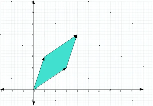
Example 4. Consider the following infeasible IP problem.
186 ≤ 33x1+ 37x2 ≤197
0 ≤ x1, x2, ≤6
x1, x2 ∈Z.
(2.3.40)
Its LP relaxation is depicted on the first picture in Figure 2.3. Branching onxi creates6 branch and
bound nodesxi = 0, . . . ,5fori= 1,2. On the other hand, branching onx1+x2proves the infeasibility
of the problem at the root node; since the minimum and the maximum ofx1+x2over the LP relaxation
of2.3.40are5.027and5.970, respectively.
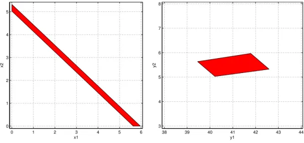
problem:
186 ≤ 4y1+ 5y2 ≤197
0 ≤ −y1+ 8y2 ≤6
0 ≤ y1−7y2 ≤6
y1, y2∈Z.
(2.3.41) Here A= 33 37 1 0 0 1
, U =
−1 8
1 −7
, AU = 4 5
−1 8
1 −7 .
The LP relaxation of the reformulated problem2.3.41is depicted in the second picture in Figure 2.3.
The second picture clearly shows that branching on y2 immmediately proves the infeasibility of the
problem. The minimum and the maximum ofy2 over the LP relaxation of2.3.41are again5.027 and
5.970, respectively.
Letui1, . . . , uinbe the rows ofU−1. It can be shown that branching onyn, . . . , y1 in this order in (IP-R) is equivalent to branching on uinx, . . . , ui1x in this order in (IP) (i.e., the two B&B trees are isomorphic).
In Example4, we have
U−1= 7 8 1 1 ,
CHAPTER 3
Unifying LLL Inequalities
Several concepts of reducedness of a lattice basis are known. The most widely used one is LLL reducedness (for details, see Section2.2.1), developed in the seminal paper [35] of Lenstra, Lenstra and Lov´asz. The quality of an LLL basis is expressed by three fundamental inequalities, (2.2.15)-(2.2.17). Surveys and textbook treatments of lattice basis reduction can be found in [20], [26], [47], and [42].
Improvements of the running time of the LLL algorithm were given, see for example Schnorr [45]. It is natural to ask, whether the three beautiful inequalities (2.2.15)-(2.2.17) can be unified and generalized: for instance, whether the product of the norms of the first few basis vectors can be bounded in terms ofdetL,or if the norm of the first basis vector can be bounded by other parameters ofL.
In this chapter we find unifying inequalities.
3.1
Generalizations of the Fundamental Inequalities in LLL Reduced
Bases
Our Theorems1and2generalize inequalities (2.2.15) through (2.2.17).
Theorem 1. Letb1, . . . , bn ∈ Rm be an LLL-reduced basis of the latticeL, andd1, . . . , dkarbitrary
linearly independent vectors inL. Then
kb1k · · · kbkk ≤ 2k(n−1)/4(detL)k/n. (3.1.5)
In the most general setting, we prove:
Theorem 2. Letb1, . . . , bn ∈ Rm be an LLL-reduced basis of the latticeL,1 ≤ k ≤ j ≤ n, and
d1, . . . , dj arbitrary linearly independent vectors inL. Then
detL(b1, . . . , bk) ≤ 2k(n−j)/2+k(j−k)/4(detL(d1, . . . , dj))k/j, (3.1.6) kb1k · · · kbkk ≤ 2k(n−j)/2+k(j−1)/4(detL(d1, . . . , dj))k/j. (3.1.7)
By settingkandjto either 1orn, from (3.1.6) we can recover the first two LLL inequalities, and from (3.1.7) we can recover all three.
The main tool is Lemma3.1.8, which may be of independent interest. Fork = 1 we can recover from it Lemma (5.3.11) in [20] (proven as part of Proposition (1.11) in [35]). First, note that ifb1, . . . , bn are linearly independent vectors, then
detL(b1, . . . , bn) = detL(b1, . . . , bn−1)kb′k, (3.1.8)
whereb′is the projection ofbnon the orthogonal complement of the linear span ofb1, . . . , bn−1.
Lemma 2. Letd1, . . . , dkbe linearly independent vectors from the lattice L,andb∗1, . . . , b∗n the Gram
Schmidt orthogonalization of an arbitary basis. Then
detL(d1, . . . , dk)≥ min 1≤i1<···<ik≤n
kb∗
i1k. . .kb
∗
ikk . (3.1.9)
Proof of Lemma2 We need the following
Claim There are elementary column operations performed ond1, . . . , dk that yieldd¯1, . . . ,d¯kwith
¯ di =
ti
X
j=1
whereλij ∈Z, λi,ti 6= 0,and
tk> tk−1>· · ·> t1. (3.1.11)
Proof of Claim Let us write
BV = [d1, . . . , dk], (3.1.12)
with V an integral matrix. Analogously to how the Hermite Normal Form of an integral matrix is computed, we can do elementary column operations onV to obtainV¯ with
tk:= max{i|v¯ik = 06 } > tk−1 := max{i|v¯i,k−1 6= 0} > . . . > t1 := max{i|v¯i16= 0}.
(3.1.13) Performing the same elementary column operations ond1, . . . , dkyieldd1, . . . ,¯ d¯k which satisfy
BV¯ = [ ¯d1, . . . ,d¯k], (3.1.14)
so they satisfy (3.1.10).
End of proof of Claim
Obviously
det L( ¯d1, . . . ,d¯k) = det L(d1, . . . , dk). (3.1.15)
Substituting from (2.2.9) forbiwe can rewrite (3.1.10) as
¯ di =
ti
X
j=1 λ∗
ijb∗j fori= 1, . . . , k, (3.1.16)
where theλ∗
ij are now reals, butλ∗i,ti =λi,tinonzero integers.
For alliwe have
span{d¯1, . . . ,d¯i−1} ⊆ span{b∗1, . . . , b ∗ ti
−1}. (3.1.17)
Therefore
kProj{d¯i| {d¯1, . . . ,d¯i−1}⊥} k ≥ kProj{d¯i| {b∗1, . . . , b∗ti
−1}
⊥
}k ≥ kλi,tib
∗ tik ≥ kb
∗
holds, with the second inequality coming from (3.1.11). HereProj{d¯i| {d¯1, . . . ,d¯i−1}⊥}is the pro-jection ofd¯iorthogonal tospan{d¯1, . . . ,d¯i−1}. So applying (3.1.8) repeatedly we get
det L( ¯d1, . . . ,d¯k) ≥ detL( ¯d1, . . . ,d¯k−1)kb∗tkk
. . .
≥ kb∗ t1kkb
∗
t2k. . .kb
∗ tkk,
(3.1.19)
which together with (3.1.15) completes the proof.
3.2
Proofs of Theorem 1 and Theorem 2
The plan of the proof is as follows: we first prove (3.1.1) through (3.1.3) in Theorem 1. Then we prove Theorem 2. Finally, (3.1.4) follows as a special case of (3.1.7) withj=k; and (3.1.5) as a special case of (3.1.7) withj=n.
Proof of (3.1.1) and (3.1.2) Lemma2implies
det L(d1, . . . , dk) ≥ kb∗t1kkb
∗
t2k. . .kb
∗
tkk (3.2.20)
for somet1, . . . , tk∈ {1, . . . , n}distinct indices. Clearly
t1+· · ·+tk≤kn−k(k−1)/2 (3.2.21)
holds. Applying first (2.2.14), then (3.2.21) yields
(det L(d1, . . . , dk))2 ≥ kb∗1k2 2(1−t1). . .kb∗1k2 2(1−tk)
= kb∗
1k2k 2k−(t1+···+tk)
≥ kb1k2k 2k(k+1)/2−kn,
which is equivalent to (3.1.1). Similarly,
(det L(d1, . . . , dk))2 ≥ kb∗1k2 2(1−t1) kb∗2k22(2−t2). . .kb∗kk2 2(k−tk)
= kb∗
1k2 . . .kb∗kk2 2(1+···+k)−(t1+···+tk) ≥ kb∗
1k2 . . .kb∗kk2 2k(k−n),
(3.2.23)
which is equivalent to (3.1.2).
Proof of (3.1.3) The proof is by induction. Let us writeDk = (detL(b1, . . . , bk))2. Fork =n−1, multiplying the inequalities
kb∗ik2≤ 2n−i kb∗nk2 (i= 1, . . . , n−1) (3.2.24)
gives
Dn−1 ≤ 2n(n−1)/2(kb∗nk2)n−1 (3.2.25) = 2n(n−1)/2
Dn Dn−1
n−1
, (3.2.26)
and after simplifying, we get
Dn−1 ≤ 2(n−1)/2(Dn)1−1/n. (3.2.27)
Suppose that (3.1.3) is true fork ≤ n−1; we will prove it fork−1. Since b1, . . . , bkforms an LLL-reduced basis ofL(b1, . . . , bk)we can replacenbykin (3.2.27) to get
Dk−1 ≤ 2(k−1)/2(Dk)(k−1)/k. (3.2.28)
By the induction hypothesis,
from which we obtain
(Dk)(k−1)/k ≤ 2(k−1)(n−k)/2(Dn)(k−1)/n. (3.2.30)
Using the upper bound on(Dk)(k−1)/kfrom (3.2.30) in (3.2.28) yields
Dk−1 ≤ 2(k−1)/22(k−1)(n−k)/2(Dn)(k−1)/k (3.2.31) = 2(k−1)(n−(k−1))/2(Dn)(k−1)/n, (3.2.32)
as required.
Proof of Theorem 2 From (3.1.3) and (3.1.2) we have
detL(b1, . . . , bk) ≤ 2k(j−k)/4(detL(b1, . . . , bj))k/j, (3.2.33) detL(b1, . . . , bj) ≤ 2j(n−j)/2detL(d1, . . . , dj). (3.2.34)
Raising (3.2.34) to the power ofk/j gives
(detL(b1, . . . , bj))k/j ≤ 2k(n−j)/2det(L(d1, . . . , dj))k/j, (3.2.35)
and plugging (3.2.35) into (3.2.33) proves (3.1.6). It is shown in [35] that
kbik2 ≤ 2i−1 kb∗ik2 for i= 1, . . . , n. (3.2.36)
Multiplying these inequalities fori= 1, . . . , k yields
kb1k · · · kbkk ≤ 2k(n−1)/4detL(b1, . . . , bk), (3.2.37)
3.3
Discussion
The kth successive minimum of L is the smallest real number t, such that there are k linearly independent vectors inLwith length bounded byt. It is denoted byλk(L). With the same setup as for (2.2.15)-(2.2.17) it is shown in [35] that
kbik ≤ 2n−1λi(L)fori= 1, . . . , n. (3.3.38)
For KZ and block KZ bases similar results were shown in [32] and [46], respectively.
The successive minimum results (3.3.38) give a more global view of the lattice and the reduced basis, than (2.2.15) through (2.2.17). Our Theorem2is similar in this respect, but it seems to be independent of (3.3.38). Of course, multiplying the latter fori= 1, . . . , k gives an upper bound onkb1k · · · kbkk, but in different terms.
The quantitiesdetL(b1, . . . , bk)andkb1k. . .kbkkare also connected by
detL(b1, . . . , bk) = kb1k. . .kbkksinθ2. . .sinθk, (3.3.39)
CHAPTER 4
Branching on a Near Parallel Integral Vector in a Knapsack
Problem
The knapsack problem is one of the most studied problems in combinatorial optimization and has many real life applications. In this chapter, we show that in a knapsack feasibility problem an integral vectorpwhich is near parallel to the constraint vectoragives a branching direction with small integer width. This result is used to analyze the rangespace and the nullspace reformulations of the knapsack problem. We prove an upper bound on the integer width along the last variable in the reformulated problems, which becomes 1when the density is sufficiently small, i.e., whenkakis sufficiently large (for a formal definition of the density of a knapsack problem, see Section5.2). The proof ingredients may be of independent interest. We extract, from the transformation matrices, an integral vector which is near parallel to the constraint vectora. The near parallel vector is a good branching direction in the original problem and a transference result shows that the last variable is a good branching direction in the reformulations.
4.1
Reformulations of the Knapsack Problem
The goal of this chapter is to analyze these reformulations on the knapsack feasibility problem
β1 ≤ ax ≤ β2
0 ≤ x ≤ v
x∈Zn,
(KP)
whereais a positive, integral row vector,β1 andβ2 are integers, without assuming any structure on the constraint vector a priori. We will assume only thatkakis large – in fact, a key point will be that the large norm implies a decomposable structure, and this structure is automatically “discovered” by the reformulations.
The rangespace reformulation of (KP) is
β1 ≤ aU y ≤ β2
0 ≤ U y ≤ v
y∈Zn,
(KP-R)
whereU is a unimodular matrix that makes the columns of
a
I
U reduced in the LLL-sense (we do not analyze it with KZ reduction). The nullspace reformulation is
−xβ ≤ V λ ≤v−xβ
λ ∈ Zn−m,
(KP-N)
where xβ ∈ Zn, axβ = β,{V λ|λ ∈ Zn−m} = N(a) and the columns ofV are reduced in the LLL-sense.
Throughtout the chapter, we will assume0 ≤ β1 ≤ β2 ≤ av, and that the gcd of the components ofais1. For a rational vectorb we denote byround(b) the vector obtained by rounding the components ofb.
For ann-vectora, we will write
f(a) = 2n/4/kak1/n,
4.2
Main Results
In this section, we will review the main results of the chapter, give some examples, explanations, and some proofs that show their connection.
The main purpose of this section is an analysis of the reformulation methods. This is done in Theorem3, which proves an upper bound on the number of B&B nodes, when branching on the last variable in the reformulations.
Theorems 4 and 5 show that an integral vector p, which is “near parallel” to acan be extracted from the transformation matrices of the reformulations. The notion of near parallelness that we use is stronger than just requiringsin(a, p) to be small. The relationship of the two parallelness concepts is clarified in Proposition2.
Theorem6proves an upper bound oniwidth(p,(KP)), wherepis an integral vector. A novelty of the bound is that it does not depend onβ1 andβ2, only on their difference. We show through examples that this bound is quite useful whenp is a near parallel vector found according to Theorems4and5.
In the end, a transference result between branching directions in the original, and reformulated problems completes the proof of Theorem3.
Theorem 3. Supposekak ≥ 2(n/2+1)n. Then
(1) iwidth(en, (KP-R)) ≤ ⌊f(a)(2kvk+(β2−β1))⌋+ 1.
(2) iwidth(en−1, (KP-N)) ≤ ⌊2g(a)kvk⌋+ 1.
Givenaandpintegral vectors, we will need the notion of their near parallelness. The obvious thing would be to require that|sin(a, p)|is small. Instead, we will write a decomposition
a=λp+r, withλ∈Q, r ∈Qn, r⊥p, (DECOMP)
and ask for krk /λ to be small. The following proposition clarifies the connection of the two near parallelness concepts and shows two useful consequences of the latter one.
Proposition 2. Suppose thata, p ∈ Zn,andrandλare defined to satisfy (DECOMP). Assume w.l.o.g.
λ >0.Then
(2) For anyM there existsa, p withkak≥M such that the inequality in (1) is strict.
(3) Denote bypi andai theith component ofp anda.Ifkrk/λ <1, andpi 6= 0, then the signs of
pi andai agree. Also, ifkrk/λ <1/2,then⌊ai/λ⌉=pi.
Proof Statement (1) follows from
sin(a, p) = krk/kak ≤ krk/kλpk ≤ krk/λ, (4.2.2)
where in the last inequality we used the integrality ofp. To see (2), consider the family ofa andp vectors
a =
m2+ 1, m2
,
p =
m+ 1, m
(4.2.3)
withman integer. Lettingλ andr be defined as in the statement of the proposition, a straightforward computation (or experimentation) shows that asm→ ∞
sin(a, p) → 0,
krk/λ → 1/√2.
Statement (3) is straightforward from
ai/λ = pi+ri/λ. (4.2.4)
The next two theorems show how the near parallel vectors can be found from the transformation matrices of the reformulations.
Theorem 4. Supposekak ≥ 2(n/2+1)n. LetU be a unimodular matrix such that the columns of
a
I
are LLL-reduced andpthe last row ofU−1. Definer andλto satisfy (DECOMP), and assume w.l.o.g.
λ >0.
Then
(1) kpk(1+krk2)1/2 ≤kakf(a);
(2) λ≥1/f(a);
(3) krk/λ≤2f(a).
Theorem 5. Supposekak ≥ 2(n/2+1)n. LetV be a matrix whose columns are an LLL-reduced basis
ofN(a),ban integral column vector withab= 1, andpthe(n−1)strow of(V, b)−1. Definerandλ
to satisfy (DECOMP), and assume w.l.o.g. λ >0.
Thenr 6= 0, and
(1) kpkkrk≤kakg(a);
(2) krk/λ≤2g(a).
It is important to note thatp is integral, butλandr may not be. Also, the measure of parallelness toa, i.e., the upper bound onkrk/λ is quite similar for thepvectors found in Theorems4and5, but their length can be quite different. Whenkakis large, thepvector in Theorem4 is guaranteed to be much shorter thana by λ ≥1/f(a). On the other hand, thepvector from Theorem 5may be much
longer thana:the upper bound onkpkkrk does not guarantee any bound onkpk, sincer can be fractional.
The following example illustrates this:
Example 5. Consider the vector
a =
3488, 451, 1231, 6415, 2191
We computedp1, r1, λ1 according to Theorem4:
p1 =
62, 8, 22, 114, 39
,
r1 =
0.2582, 0.9688, −6.5858, 2.0554, −2.9021
,
λ1 = 56.2539,
kr1k/λ1 = 0.1342.
(4.2.6)
We also computedp2, r2, λ2 according to Theorem5; notekp2k>kak:
p2 =
12204, 1578, 4307, 22445, 7666
r2 =
−0.0165, −0.0071, 0.0194, 0.0105, −0.0140
λ2 = 0.2858
kr2k/λ2 = 0.1110.
(4.2.7)
Theorem6below gives an upper bound on the number of B&B nodes when branching on a hyper-plane in (KP).
Theorem 6. Suppose thata=λp+r, withp≥0.Then
iwidth(p,(KP)) ≤
krkkvk λ +
β2−β1 λ
+ 1. (4.2.8)
This bound is quite strong for near parallel vectors computed from Theorems4and5. For instance, leta, p1, r1, λ1 be as in Example5. Ifβ1 =β2 in a knapsack problem with weight vectoraand each xi is bounded between 0and 3, then Theorem 6implies that the integer width is at most one. At the other extreme, it also implies that the integer width is at most one, if eachxi is bounded between0and 1, andβ2−β1 ≤39. However, this bound does not seem as useful, whenpis a “simple” vector, say a unit vector. Note that the assumption thatp≥0is only to simplify the proofs.
We now complete the proof of Theorem3, based on a simple transference result between branching directions, taken from [31].
Let us denote byQ, QR, andQN the feasible sets of the LP relaxations of (KP), of (KP-R), and of (KP-N), respectively.
First, letU andpbe the transformation matrix, and the near parallel vector from Theorem4. It was shown in [31] thatiwidth(p, Q) = iwidth(pU, QR). ButpU =±en, so
iwidth(p, Q) = iwidth(en, QR). (4.2.9)
On the other hand,
iwidth(p, Q) ≤
krkkvk λ +
β2−β1 λ
+ 1
≤ ⌊f(a)(2kvk+(β2−β1))⌋+ 1
(4.2.10)
with the first inequality coming from Theorem 6 and the second from using the bounds on1/λ and krk/λ from Theorem4. Combining (4.2.9) and (4.2.10) yields (1) in Theorem3.
Now letV andpbe the transformation matrix, and the near parallel vector from Theorem5. It was shown in [31] thatiwidth(p, Q) = iwidth(pV, QN).ButpV =±en−1, so
iwidth(en−1, QN) = iwidth(p, Q). (4.2.11)
On the other hand,
iwidth(p, Q) ≤
krkkvk λ
+ 1
≤ ⌊g(a)(2kvk)⌋+ 1.
(4.2.12)
with the first inequality coming from Theorem6and the second from using the bound onkrk /λ in Theorem5. Combining (4.2.11) and (4.2.12) yields (2) in Theorem3.
4.3
Near Parallel Vectors: Intuition and Proofs of Theorems
4
and
5
Proof of Theorem4 First note that the lower bound onkakimplies
LetLℓbe the lattice generated by the firstℓcolumns of a I U,and
Z =
0 U−1
1 −a
.
Clearly,Z is unimodular and
Z aU U = In 01×n
. (4.3.14)
So Lemma1implies thatLℓis complete and the lastn+ 1−ℓrows ofZgenerateL⊥ℓ . The last row of Zis(1,−a) and the next-to-last is(0, p), so we get
detLn = detL⊥n = (kak2 +1)1/2,
detLn−1 = detL⊥n−1 =kpk(1+krk2)1/2.
(4.3.15)
(3.1.3) of Theorem1implies
detLn−1 ≤ 2(n−1)/4(detLn)1−1/n. (4.3.16)
Substituting into (4.3.16) from (4.3.15) gives
kpk(1+krk2)1/2 ≤ 2(n−1)/4(pkak2 +1)1−1/n
≤ 2n/4 kak1−1/n
= kakf(a),
(4.3.17)
Proof of (2) From (1) we directly obtain
f(a)2kak2− krk2
kpk2 ≥
f(a)2 kak2 − kpk2krk2 kpk2
≥ 1
= f(a) 2 kak2 f(a)2 kak2,
(4.3.18)
where in the first inequality we usedkpk≥1. Now note
kpk2≤f(a)2 kak2,
i.e., the the denominator of the first expression in (4.3.18) is not larger than the denominator of the last expression. So if we replacef(a)2by1in the numerator of both, the inequality will remain valid. The result is
kak2− krk2 kpk2 ≥
1
f(a)2, (4.3.19)
which is the square of the required inequality.
Proof of (3) We have
krk2 λ2 ≤
kpk2krk2 kλpk2
= kpk 2krk2 kak2 − krk2
≤ f(a) 2 kak2 kak2 − krk2
≤ f(a) 2 kak2 kak2 −f(a)2kak2
= f(a) 2
1−f(a)2
≤ 4f(a)2,
(4.3.20)
Proof of Theorem5 The lower bound onkakimplies
g(a)≤√3/2. (4.3.21)
LetLℓbe the lattice generated by the firstℓcolumns ofV.We have
(V, b)−1V =
In−1
0
. (4.3.22)
So Lemma1implies thatLℓis complete and the lastn−ℓrows of(V, b)−1generateL⊥ℓ . It is elementary to see that the last row of(V, b)−1 isaand by definition the next-to-last row isp,and these rows are independent, sor6= 0.Also,
detLn−1 = detL⊥n−1 =kak,
detLn−2 = detL⊥n−2 =kpkkrk.
(4.3.23)
(3.1.3) of Theorem1withn−1in place ofn andn−2in place ofkimplies
det Ln−2 ≤ 2(n−2)/4(detLn−1)1−1/(n−1). (4.3.24)
Substituting into (4.3.24) from (4.3.23) gives
kpkkrk ≤ 2(n−2)/4 kak1−1/(n−1)
= kakg(a),
(4.3.25)
as required.
4.4
Branching on a Near Parallel Vector: Proof of Theorem
6
This proof is somewhat technical, so we state and prove some intermediate claims, to improve readability. Let us fixa, p, β1, β2,andv. For a row-vectorw and an integerℓ we write
max(w, ℓ) = max{wx|px≤ℓ,0≤x≤v}
min(w, ℓ) = min{wx|px≥ℓ,0≤x≤v}.
(4.4.26)
The dependence on p, on v and on the sense of the constraint (i.e., ≤ or ≥) is not shown by this notation; however, we always usepx≤ℓ with “max” andpx≥ℓ with “min”, andp andvare fixed. Note that asais a row-vector andva column-vector,avis their inner product, and the meaning ofpvis similar.
Claim 1. Suppose thatℓ1andℓ2are integers in{0, . . . , pv}.Then
min(a, ℓ2)−max(a, ℓ1) ≥ − krkkvk+λ(ℓ2−ℓ1). (4.4.27)
Proof The decomposition ofashows
max(a, ℓ1) ≤ max(r, ℓ1) +λℓ1, and min(a, ℓ2) ≥ min(r, ℓ2) +λℓ2.
(4.4.28)
So we get the following chain of inequalities, with ensuing explanation:
min(a, ℓ2)−max(a, ℓ1) ≥ min(r, ℓ2)−max(r, ℓ1) +λ(ℓ2−ℓ1)
≥ rx2−rx1+λ(ℓ2−ℓ1)
= r(x2−x1) +λ(ℓ2−ℓ1)
≥ − krkkvk+λ(ℓ2−ℓ1).
(4.4.29)
Herex2andx1are the solutions that attain the maximum and the minimum inmin(r, ℓ2)andmax(r, ℓ1), respectively. The last inequality follows from the fact that theith component ofx2−x1 is at mostviin absolute value and the Cauchy-Schwartz inequality.
Next, let us note
min(a, k) ≤ max(a, k) fork∈ {0, . . . , pv}. (4.4.30)
Indeed, (4.4.30) holds, since the feasible sets of the optimization problems defining min(a, k) and max(a, k) contain{x|px=k,0≤x≤v}.
The nonnegativity ofp and ofa implymin(a,0) = 0and max(a, pe) =av.The proof of the following claim is trivial, hence omitted.
Claim 2. Suppose thatℓ1andℓ2are integers in{0, . . . , pv}withℓ1+ 1≤ℓ2 and
max(a, ℓ1)< β1 ≤β2 <min(a, ℓ2). (4.4.31)
Then for allx withβ1 ≤ax≤β2,0≤x≤v
ℓ1< px < ℓ2 (4.4.32)
holds.
We assume for simplicity
max(a,0)< β1 ≤β2 <min(a, pe); (4.4.33)
the cases when this fails to hold are easy to handle separately. Letℓ1be the largest andℓ2 the smallest integer such that
max(a, ℓ1)< β1 ≤β2 <min(a, ℓ2). (4.4.34)
From (4.4.30)ℓ2 ≥ℓ1+ 1 follows and Claim2yields
iwidth(p, (SU B)) ≤ ℓ2−ℓ1−1. (4.4.35)
By the choices ofℓ1 andℓ2 we have
hence Claim1leads to
β2−β1 ≥ min(a, ℓ2−1)−max(a, ℓ1+ 1)
≥ − krkkvk+λ(ℓ2−ℓ1−2),
(4.4.37)
that is
ℓ2−ℓ1−2 ≤
β2−β1 λ +
krkkvk
λ . (4.4.38)
Comparing (4.4.35) and (4.4.38) completes the proof.
4.5
Successive Approximation
Theorems 4and 5approximate aby a single vector. It is natural to ask: if one row ofU−1, or of (V, b)−1is a good approximation ofa, can we construct a better approximation from2,3, . . . , k rows? The answer is yes and we outline the corresponding results below, and their proofs, which are slight modifications of the proofs of Theorems 4and 5. As of now, we don’t know how to use the general results for a better analysis of the reformulations than what is already given in Theorem3.
So we mainly state the successive approximation results for the interesting geometric intuition they give. Let us define
f(a, k) = 2(k(n−k)+1)/4/kakk/n,
g(a, k) = 2k(n−1−k)/4/kak(k−1)/n .
(4.5.39)
The successive version of Theorem4is given below:
Theorem 7. Leta∈Zn be a row-vector, withkak≥2(n/2+1)n, U a unimodular matrix such that the
columns of
a
I
U
are LLL-reduced andPk the (integral) submatrix ofU−1consisting of the lastkrows. Furthermore, let
a(k)be the projection ofaonto the subspace spanned by the rows ofPk, r=a−a(k) and