Block Krylov Subspace Spectral Methods for Variable-Coefficient Elliptic PDE

Block Krylov Subspace Spectral Methods for

Variable-Coefficient Elliptic PDE

James V. Lambers

Abstract—Krylov subspace spectral (KSS) methods have been demonstrated to be effective tools for solv-ing time-dependent variable-coefficient PDE. They employ techniques developed by Golub and Meurant for computing elements of functions of matrices to approximate each Fourier coefficient of the solution using a Gaussian quadrature rule that is tailored to that coefficient. In this paper, we apply this same ap-proach to time-independent PDE of the formLu=f, whereLis an elliptic differential operator. Numerical results demonstrate the effectiveness of this approach for Poisson’s equation and the Helmholtz equation in two dimensions.

Keywords: spectral methods, Gaussian quadrature, block Lanczos method, Poisson’s equation, Helmholtz equation

1

Introduction

Let Lbe an elliptic second-order differential operator of the form

Lu=−∇ ·(p∇u) +qu, (1)

where p(x, y)>0 andq(x, y) are smooth functions. We consider the following boundary value problem on a rect-angle,

Lu=g(x, y), 0< x, y <2π, (2)

with homogeneous Dirichlet boundary conditions, or pe-riodic boundary conditions.

In [12] a class of methods, called Krylov subspace spectral (KSS) methods, was introduced for the purpose of solv-ing parabolic variable-coefficient PDE. These methods are based on techniques developed by Golub and Meu-rant in [3] for approximating elements of a function of a matrix by Gaussian quadrature in thespectraldomain. In [6, 8], these methods were generalized to the second-order wave equation, for which these methods have exhibited even higher-order accuracy.

It has been shown in these references that KSS meth-ods, by employing different approximations of the solu-tion operator for each Fourier coefficient of the solusolu-tion, achieve higher-order accuracy in time than other Krylov

∗_{Submitted March 20, 2009. Stanford University, Department}

of Energy Resources Engineering, Stanford, CA 94305-2220 USA Tel/Fax: 650-725-2729/2099 Email: [email protected]

subspace methods (see, for example, [7]) for stiff systems of ODE, and, as shown in [8], they are also quite stable, considering that they are explicit methods. In [9, 10], the accuracy and robustness of KSS methods were enhanced using block Gaussian quadrature. Recent extensions in-clude the time-dependent Schr¨odinger equation [11] and Maxwell’s equations [14].

It is our hope that by a change of integrand in the in-tegrals used to compute the Fourier coefficients of the solution, the high accuracy achieved for time-dependent problems can be extended to the time-independent case, even for cases in which the operator L is indefinite, as in the Helmholtz equation. Section 2 reviews the main properties of KSS methods, including block KSS meth-ods, and explains how they can be applied to elliptic prob-lems. Numerical results are presented in Section 3, and conclusions are stated in Section 4.

2

Krylov Subspace Spectral Methods

We first review KSS methods, which were first developed in [12] for parabolic problems. Let S = L−1 represent the exact solution operator of the problem (2), restricted to one space dimension for simplicity, and let·,·denote the standard inner product of functions defined on [0,2π],

u(x), v(x)= 2π

0 u(x)v(x)dx. (3)

Krylov subspace spectral methods, introduced in [12], use Gaussian quadrature on the spectral domain to compute the Fourier coefficients of the solution. Given the right-hand sideg(x), the solution is computed by approximat-ing the Fourier coefficients that would be obtained by applying the exact solution operator tog(x),

ˆ

u(ω) =

1 √

2πe

iωx_{, Sg(x). (4)}

2.1 Elements of Functions of Matrices

In [3] Golub and Meurant describe a method for comput-ing quantities of the form

uTf(A)v, (5)

goal is to apply this method with A = LN where LN is a spectral discretization of L, f(λ) = λ−1, and the vectorsuandvare derived from ˆe_ωandg, where ˆe_ω is a discretization of √1

2πeiωxandgrepresents the right-hand side functiong(x), evaluated on anN-point uniform grid.

The basic idea is as follows: since the matrix Ais sym-metric positive definite, it has real eigenvalues

b=λ₁≥λ₂≥ · · · ≥λ_N =a >0, (6)

and corresponding orthogonal eigenvectors qj, j = 1, . . . , N. Therefore, the quantity (5) can be rewritten as

uTf(A)v= N

j=1

f(λj)uTqjqTjv. (7)

We leta=λN be the smallest eigenvalue,b=λ1 be the

largest eigenvalue, and define the measure α(λ) by

α(λ) = ⎧ ⎪ ⎨ ⎪ ⎩

0, ifλ < a

N

j=iαjβj, ifλi≤λ < λi−1

N

j=1αjβj, ifb≤λ

, (8)

whereα_j=uTq_j andβ_j =qT_jv.If this measure is posi-tive and increasing, then the quantity (5) can be viewed as a Riemann-Stieltjes integral

uTf(A)v=I[f] = b

a f(λ)dα(λ). (9)

As discussed in [3], the integralI[f] can be approximated using Gaussian quadrature rules, which yield an approx-imation of the form

I[f] = K

j=1

w_jf(t_j) +R[f], (10)

where the nodestj,j = 1, . . . , K, as well as the weights

wj, j = 1, . . . , K, can be obtained using the symmetric Lanczos algorithm ifu=v, and the unsymmetric Lanc-zos algorithm ifu=v(see [5]).

2.2 Block Gaussian Quadrature

In the caseu=v, there is the possibility that the weights may not be positive, which destabilizes the quadrature rule (see [1] for details). One option to get around this problem is rewriting (5) using decompositions such as

uTf(A)v= 1

δ[u

T_{f(A)(u+δv)−u}T_{f(A)u], (11)}

where δ is a small constant. Guidelines for choosing an appropriate value forδ can be found in [12, Section 2.2].

If we compute (5) using (11) or thepolar decomposition

1

4[(u+v)

T_{f(A)(u+v)−(v−u)}T_{f(A)(v−u)], (12)}

then we have to carry out the process for approximating an expression of the form (5) with two sets of starting vec-tors, whereas a single quadrature rule is more desirable. Instead, we consider

u v Tf(A) u v

which results in the 2×2 matrix b

a f(λ)dμ(λ) =

uTf(A)u uTf(A)v vTf(A)u vTf(A)v

, (13)

whereμ(λ) is a 2×2 matrix function ofλ, each entry of which is a measure of the formα(λ) from (8).

In [3] Golub and Meurant show how a block approach can be used to generate quadrature formulas. We will describe this process here in more detail. The integral b

af(λ)dμ(λ) is now a 2×2 symmetric matrix and the most generalK-node quadrature formula is of the form

b

a

f(λ)dμ(λ) = K

j=1

W_jf(T_j)W_j+error, (14)

with Tj and Wj being symmetric 2×2 matrices. By diagonalizing eachTj, we obtain the simpler formula

b

a

f(λ)dμ(λ) =

2K

j=1

f(λ_j)v_jvT_j +error, (15)

where, for eachj,λj is a scalar andvj is a 2-vector.

Each node λj is an eigenvalue of the matrix

TK= ⎡ ⎢ ⎢ ⎢ ⎢ ⎢ ⎣

M1 B1T

B₁ M₂ B₂T

. .. . .. . ..

BK−2 MK−1 BKT−1

B_K−1 M_K

⎤ ⎥ ⎥ ⎥ ⎥ ⎥ ⎦ (16)

which is a block-triangular matrix of order 2K. The vec-torvjconsists of the first two elements of the correspond-ing normalized eigenvector.

To compute the matrices Mj and Bj, we use the block Lanczos algorithm, which was proposed by Golub and Underwood in [4]. Let X0 be an N ×2 given matrix,

such thatX₁TX₁=I₂. LetX₀= 0 be anN×2 matrix. Then, for j= 1, . . . , K, we compute

M_j =X_jTAX_j,

Rj=AXj−XjMj−Xj−1BjT−1, (17)

Xj+1Bj =Rj.

The last step of the algorithm is theQRdecomposition of Rj such that Xj+1 is n×2 with XjT+1Xj+1 = I2.

2.3 Block KSS Methods

We are now ready to describe block KSS methods for elliptic PDE in 1-D of the form Lu= g. For each wave numberω=−N/2 + 1, . . . , N/2, we define

R0(ω) = ˆeω g

and compute theQRfactorizationR0(ω) =X1(ω)B0(ω).

We then carry out the block Lanczos iteration described in (17) to obtain a block tridiagonal matrixTK(ω) of the form (16), where each entry is a function ofω.

Then, we can express each Fourier coefficient of the ap-proximate solution as

[ˆu]_ω =B₀HEH₁₂[T_K(ω)]−1E₁₂B₀₁₂ (18)

where E₁₂= e₁ e₂ .The computation of (18) con-sists of computing the eigenvalues and eigenvectors of TK(ω) in order to obtain the nodes and weights for Gaus-sian quadrature, as described earlier.

Once the approximationuis computed using the inverse FFT, we can compute the residual r = g−L_Nu, and correct the solution by applying the block KSS method again to the problemLNc=r, and updating the solution by u =u+c. We can continue this process of residual correction until the residual is sufficiently small.

Although we have restricted ourselves to one space di-mension in the description of block KSS methods, gener-alization to higher dimensions is straightforward, as dis-cussed in [13].

3

Numerical Results

In this section we demonstrate the effectiveness of block KSS methods for solving elliptic PDE.

3.1 Poisson’s Equation

We first apply a 2-node block KSS method to the problem

∇ ·(p(x, y)∇u(x, y)) =g(x, y), 0< x, y <2π, (19)

with Dirichlet boundary conditions, where

p(x, y) ≈ 4.03 + 0.017 cosy+ 0.0052 siny+ 0.0026 cos 2y+ 0.029 cosx+ 0.014 sinx+ 0.0083 cos(x+y) + 0.0019 cos(x−2y) +

0.0073 cos(x−y) +

0.0046 sin(x−y) + 0.0021 cos 2x, (20)

g(x, y) ≈ −2.39 siny+ 1.44 sin 2y+ 0.47 sin 3y−0.31 sinx−

1.44 sin(x+y) + 0.19 sin(x+ 2y)− 5.73 sin(x−y)−0.53 sin 2x−

0.35 sin(2x+y)−

1.63 sin(2x−y) + 1.07 sin 3x+

0.6 sin(3x+y). (21)

The coefficient p(x, y) is constructed so as to have the smoothness of a function with four continuous deriva-tives, using a technique described in [12]. The function

f is obtained by applying the spatial operator Lu = −∇ ·(p∇u) to a function u(x, y) that is constructed in the same was as p(x, y), with the same smoothness, so that the exact solution is known.

In our experiments, we will use different grid spacings in order to investigate how the error varies with increasing resolution. The problem data is computed on the finest grid, and projected onto the coarser grids. However, in order to isolate error due to KSS methods themselves, we do not include error due to truncation of Fourier series in our error estimates.

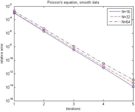
The results are shown in Figure 1 and Table 1. The relative error is rapidly reduced by residual correction until it is not much greater than machine precision. As shown in the figure, we achieve linear convergence, with a very small asymptotic error constant. We also see that the error only increases by a factor of 3 as the number of grid points per dimension doubles, but since these error estimates do not include truncation of Fourier series, it follows that the overall errordecreases as the number of grid points increases.

Figure 1: Relative error in solutions to Poisson’s equation (19), (20), (21) computed by 2-node block KSS methods with residual correction.

We now solve (19) with a less smooth coefficient and right-hand side,

Table 1: Relative L2 error, excluding truncation of Fourier series, in solutions of (19), (20), (21) withN grid points per dimension. The third column lists the number of iterations of residual correction.

N Error Iterations 16 1.3e-14 4 32 4.0e-14 4 64 1.2e-13 4

0.0021 sin 3y+ 0.029 cosx+ 0.014 sinx+ 0.0083 cos(x+y) +

0.0036 cos(x+ 2y) + 0.0023 cos(x+ 3y) + 0.0066 cos(x−2y) + 0.0073 cos(x−y) + 0.0046 sin(x−y) + 0.0072 cos 2x+ 0.0038 cos(2x+y) + 0.0018 sin(2x+y) + 0.004 cos(2x−y)−0.0034 sin(2x−y) + 0.004 cos 3x+ 0.0033 cos(3x+y) +

0.0026 cos(3x−y), (22)

g(x, y) ≈ −2.39 siny+ 4.93 sin 2y+

3.82 sin 3y−0.31 sinx−1.44 sin(x+y) + 0.68 sin(x+ 2y)−1.37 sin(x+ 3y)− 0.98 sin(x−3y)−5.75 sin(x−y)− 1.78 sin 2x−1.15 sin(2x+y)− 1.21 sin(2x+ 2y)−1.67 sin(2x+ 3y)− 0.24 sin(2x−3y) + 0.95 sin(2x−2y)− 0.12 cos(2x−y)−5.47 sin(2x−y) + 0.34 cos 3x+ 8.84 sin 3x+

0.19 cos(3x+y) + 4.95 sin(3x+y) + 2.3 sin(3x+ 2y)−1.84 sin(3x+ 3y) + 0.72 sin(3x−3y) + 0.79 sin(3x−2y) + 0.98 sin(3x−y), (23)

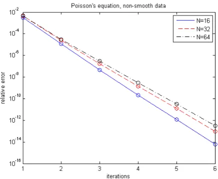
and with Dirichlet boundary conditions. The results are shown in Figure 2 and Table 2. We observe that even though the Fourier coefficients of the problem data decay more slowly than in the previous problem by two orders of magnitude, the computed solution has comparable ac-curacy, after just one extra iteration of residual correc-tion. As before, the error increases only moderately as the number of grid points per dimension is doubled.

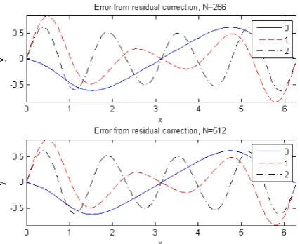
Figure 3 displays the error in solutions to a one-dimensional analogue of (19) with smoothly varying co-efficients and data, after each pass of residual correction, using a 2-node block KSS method with 256 and 512 grid points, respectively. It can easily be seen from the fig-ure, and confirmed by a simple Fourier analysis, that for Poisson’s equation, the error in the initial iterations of residual correction is smooth, but becomes less smooth as residual correction continues. Furthermore, the initial

Figure 2: Relative error in solutions to Poisson’s equation (19), (22), (23) computed by 2-node block KSS methods with residual correction.

Table 2: Relative L2 error, excluding truncation of Fourier series, in solutions of (19), (22), (23) withNgrid points per dimension. The third column lists the number of iterations of residual correction.

N Error Iterations 16 6.0e-15 5 32 8.9e-14 5 64 3.1e-13 5

smooth error is essentially independent of the grid reso-lution. Therefore, it makes sense to use a multigrid-like approach, in which initial solutions are computed on a coarse grid, and corrected on a finer grid; that is, the opposite sequence of a traditional V-cycle. Future work will explore the development of more efficient iterative methods based on this idea.

3.2 The Helmholtz Equation

Now, we apply a 2-node block KSS method to the inho-mogeneous Helmholtz equation

Δu(x, y) +k(x, y)2u(x, y) =g(x, y), (24)

with periodic boundary conditions, where

k(x, y)2 ≈ 4.03 + 0.017 cosy+ 0.0052 siny+ 0.029 cosx+ 0.014 sinx+

0.0083 cos(x+y) + 0.0073 cos(x−y) + 0.0046 sin(x−y), (25)

g(x, y) ≈ 1.63 + 0.015 cosy+ 0.0039 siny+ 0.014 cosx+ 0.0057 sinx+

Figure 3: Error in computed solutions to a 1-D ana-logue of (19) after zero (solid blue curve), one (dashed red curve), two (dotted-dashed black curve) and three (dotted green curve) iterations of residual correction in conjunction with a 2-node block KSS method on a 256-point grid (top plot) and a 512-256-point grid (bottom plot).

0.0033 sin(x−y). (26)

The results are shown in Table 3. Although the solution is not as accurate as for Poisson’s equation, we note that the accuracy does not degrade with the number of grid points. This is due to the fact that the dominant portion of the error arises from the computation of the Fourier coefficients corresponding to the region of phase space where the symbol ofL= Δ +k2 is smallest. This leads to Gaussian quadrature nodes near the singularity in the integrand f(λ) = λ−1. The integrand is more difficult to approximate accurately by polynomial interpolation near this singularity, and the resulting error is negligibly impacted by the grid refinement.

However, this error is substantially reduced if the coeffi-cientk(x, y)2and right-hand sideg(x, y) are very smooth, because then the basis functions eiω·x are nearly eigen-functions, which makes most of the terms αjβj in (8) negligibly small. Future work will explore the use of pre-conditioning similarity transformations, aided by fast al-gorithms presented in [2] for application of Fourier inte-gral operators, for homogenizing variable coefficients in order to improve the performance of KSS methods for such problems.

We now solve the modified problem

Δu(x, y) + 100k(x, y)2u(x, y) =g(x, y), (27)

with periodic boundary conditions andk(x, y) andg(x, y) as defined in (25), (26). The results are listed in Table 4. We see that even though there is a greater degree

Table 3: Relative L2 error, excluding truncation of Fourier series, in solutions of (24), (25), (26) withNgrid points per dimension. The third column lists the number of iterations of residual correction.

N Error Iterations 16 3.5e-9 5 32 3.5e-9 5 64 3.5e-9 5

of indefiniteness in the operator L, the errors are still quite small, and that high accuracy is achieved after only a single residual correction. This is because the domi-nant portion of the error, described earlier, corresponds to Fourier coefficients that, in the exact solution, are sig-nificantly smaller.

Table 4: Relative L2 error, excluding truncation of Fourier series, in solutions of (27), (25), (26) withNgrid points per dimension. The third column lists the number of iterations of residual correction.

N Error Iterations 16 1.9e-16 1 32 9.7e-15 1 64 1.3e-11 1

We now solve (24) with less smooth coefficients and data,

k(x, y)2 ≈ 4.03 + 0.017 cosy+ 0.0052 siny+ 0.0026 cos 2y+ 0.029 cosx+ 0.014 sinx+ 0.0083 cos(x+y) + 0.0019 cos(x−2y) + 0.0073 cos(x−y) + 0.0046 sin(x−y) + 0.0021 cos 2x, (28)

g(x, y) ≈ 1.62 + 0.015 cosy+ 0.0039 siny+ 0.0011 cos 2y+ 0.014 cosx+ 0.0057 sinx+ 0.0048 cos(x+y) +

0.0056 cos(x−y) + 0.0033 sin(x−y),(29)

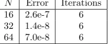
and with periodic boundary conditions. The results are shown in Table 5. We observe that as before, the error is relatively insensitive to increases in the number of grid points per dimension, although the reduced smoothness does cause this error to increase to a small extent.

Table 5: Relative L2 error, excluding truncation of Fourier series, in solutions of (24), (28), (29) withN grid points per dimension. The third column lists the number of iterations of residual correction.

N Error Iterations 16 2.6e-7 6 32 1.4e-8 6 64 7.0e-8 6

to higher frequencies than when k2 is relatively small, higher-frequency oscillations are introduced, which are then amplified by differentiation during the computation of the recursion coefficients inTK, resulting in larger er-rors.

Table 6: Relative L2 error, excluding truncation of Fourier series, in solutions of (27), (28), (29) withN grid points per dimension. The third column lists the number of iterations of residual correction.

N Error Iterations 16 3.0e-14 1 32 8.4e-12 1

64 4.5e-5 1

4

Summary and Future Work

We have demonstrated that KSS methods, while origi-nally designed for time-dependent PDE, can also be ap-plied to time-independent elliptic PDE with smoothly varying coefficients. Using residual correction, these methods can compute highly accurate solutions, even for the Helmholtz equation, for which the integrand in the Riemann-Stieltjes integrals used to compute Fourier co-efficients is singular.

Future work will extend the approach described in this paper to problems in which the coefficients and data are oscillatory or discontinuous, and problems featuring com-plicated geometry. In addition, we will consider the use of Gauss-Radau and Gauss-Lobatto rules, in which selected nodes are prescribed, to deal with the singularity associ-ated with the Helmholtz equation. We will also explore the development of multigrid-like approaches to residual correction in order to maximize efficiency.

References

[1] Atkinson, K.: An Introduction to Numerical Analy-sis, 2nd Ed.Wiley (1989)

[2] Candes, E., Demanet, L., Ying, L.: Fast Compu-tation of Fourier Integral Operators. SIAM J. Sci. Comput.29(6) (2007) 2464-2493.

[3] Golub, G. H., Meurant, G.: Matrices, Moments and Quadrature.Proceedings of the 15th Dundee Confer-ence, June-July 1993, Griffiths, D. F., Watson, G. A. (eds.), Longman Scientific & Technical (1994)

[4] Golub, G. H., Underwood, R.: The block Lanc-zos method for computing eigenvalues.Mathematical Software III, J. Rice Ed., (1977) 361-377.

[5] Golub, G. H, Welsch, J.: Calculation of Gauss Quadrature Rules.Math. Comp.23(1969) 221-230.

[6] Guidotti, P., Lambers, J. V., Sølna, K.: Analysis of 1-D Wave Propagation in Inhomogeneous Media.

Numerical Functional Analysis and Optimization27 (2006) 25-55.

[7] Hochbruck, M., Lubich, C.: On Krylov Subspace Approximations to the Matrix Exponential Opera-tor.SIAM Journal of Numerical Analysis34(1996) 1911-1925.

[8] Lambers, J. V.: Derivation of High-Order Spec-tral Methods for Time-dependent PDE using Modi-fied Moments.Electronic Transactions on Numerical Analysis28(2008) 114-135.

[9] Lambers, J. V.: Enhancement of Krylov Sub-space Spectral Methods by Block Lanczos Iteration.

Electronic Transactions on Numerical Analysis 31 (2008) 86-109.

[10] Lambers, J. V.: An Explicit, Stable, High-Order Spectral Method for the Wave Equation Based on Block Gaussian Quadrature.IAENG Journal of Ap-plied Mathematics38(2008) 333-348.

[11] Lambers, J. V.: Krylov Subspace Spectral Meth-ods for the Time-Dependent Schr¨odinger Equation with Non-Smooth Potentials.Numerical Algorithms

in press.

[12] Lambers, J. V.: Krylov Subspace Spectral Meth-ods for Variable-Coefficient Initial-Boundary Value Problems. Electronic Transactions on Numerical Analysis20(2005) 212-234.

[13] Lambers, J. V.: Practical Implementation of Krylov Subspace Spectral Methods. Journal of Scientific Computing32(2007) 449-476.