A Possibility Linear Programming Approach to Solve a Fuzzy Single Machine Scheduling Problem

Vol. 1, No. 2, pp 116 -129 Summer 2007

A Possibility Linear Programming Approach to Solve a Fuzzy Single

Machine Scheduling Problem

I.N. Kamalabadi1*, A.H. Mirzaei2, B. Javadi3

1

Department of Industrial Engineering, Faculty of Engineering, University of Kurdistan, Sanandaj, Iran ([email protected])

2

Department of Industrial Engineering, Faculty of Engineering, Tarbiat Modares University, P.O.Box 14115/111, Tehran, Iran

([email protected]) 3

Department of Industrial Engineering, Mazandaran University of Science and Technology, P.O.Box 734, Babol, Iran

([email protected]) ABSTRACT

This paper employs an interactive possibility linear programming approach to solve a single machine scheduling problem with imprecise processing times, due dates, as well as earliness and tardiness penalties of jobs. The proposed approach is based on a strategy of minimizing the most possible value of the imprecise total costs, maximizing the possibility of obtaining a lower total costs, and minimizing the risk of obtaining higher total costs simultaneously. This approach is applicable to just-in-time systems, in which many firms face the need to complete jobs as close as possible to their due dates. The objective of the model is to minimize the total costs of earliness/tardiness penalties. In this paper, the proposed possibility linear programming approach is applied to a fuzzy single machine scheduling problem with respect to the overall degree of decision maker satisfaction. Due to the proposed model’s complexity, conventional optimization methods cannot be utilized in reasonable time. Hence, the particle swarm optimization method is applied toward its solution.

Keywords: Single machine scheduling, Earliness / tardiness, Possibility linear programming, Particle swarm optimization.

1. INTRODUCTION

The single machine environment is the basis for other types of scheduling problems. We are to determine the sequencing of N jobs so that the system performance measures such as makespan, completion time, tardiness, number of tardy jobs, and idle times are optimized. Emergence of Just-in-Time (JIT) production philosophy forces jobs to be completed as close to their due dates as possible. Because of the holding, deterioration or opportunity costs of the early jobs, and the costs of customer compensation for missing the due date or the loss of goodwill, the lost sales and performance penalties in the JIT systems, minimizing the earliness and tardiness criteria are important.

Single machine scheduling models addressing both earliness and tardiness costs are relatively recent. Here we cite some recent research works related to earliness-tardiness cost criteria. Liaw

*

(1999) proposes a branch-and-bound approach where machine idle time is not allowed. Chang (1999) deals with a no-weighted problem without preemption. Rabadia et al. (2004) investigate the problem in which due dates of all jobs are identical and setup times depend on jobs’ sequencing. Mazzini and Armentano (2001) have developed a heuristic for minimizing total earliness and tardiness cost in a single machine scheduling problem with distinct ready times and due dates. Mondal and Sen (2001) suggest an algorithm to solve the problem with a common due date. This algorithm uses a graph search space. Wan and Yen (2002) propose an approach to combine a Tabu search (TS) procedure and an optimal timing algorithm for solving the problem with distinct due windows. Feldmann and Biskup (2003) address the restrictive common due date problem by using three meta-heuristic algorithms (evolutionary search (ES), simulated annealing (SA) and threshold accepting (TA)).Ventura and Radhakrishnan (2003) use a Lagrangian relaxation procedure that utilizes the subgradient algorithm to tackle the problem. Tavakkoli-Moghaddam et al. (2005) consider the common due date problem with the objective of minimizing the sum of maximum earliness and tardiness costs. They propose an algorithm, named idle insert algorithm, to solve this problem. Lin et al. (2006) use a sequential exchange approach to solve the common due date problem.

In the conventional scheduling problem, input data or related parameters, such as processing times, due dates, ready times and earliness and tardiness penalties have been assumed to be deterministic (Brucker, 1998). Though, in real-world scheduling problems, these parameters are often encountered with uncertainty. Accordingly, scheduling problems have been mainly branched into two categories: deterministic and non-deterministic (stochastic, fuzzy, ...) problems (Peng and Liu, 2004). In the face of uncertainty, it is more appropriate that the uncertainty be incorporated into scheduling models. One of the approaches for incorporating the uncertainty into scheduling models is fuzzy theory. As of late some papers have dealt with fuzzy treatment of scheduling problems which seems to be an interesting alternative to the deterministic and especially stochastic approaches (Chanas and Kasperski, 2001, 2003). A few of such works have focused on the single machine scheduling problem with some or all fuzzy parameters. Chanas and Kasperski (2001) have investigated this scheduling problem with fuzzy processing times and fuzzy due dates.

Their objective is to minimize maximum lateness. Lam and Cai (2002) have addressed the single machine scheduling problem with fuzzy due dates and nonlinear lateness cost functions. Their objective is minimizing the maximum lateness. Chanas and Kasperski (2003) consider two single machine scheduling problems with fuzzy processing times and fuzzy due dates. In the first problem they minimize the maximal expected value of a fuzzy tardiness and in the second they minimize the expected value of a maximal fuzzy tardiness.

In this research, the objective is minimizing the sum of weighted tardiness and earliness penalties. The proposed model considers some triangular fuzzy parameters such as processing times, due dates, and unit cost of earliness/tardiness (E/T) penalties as an extension of previous models. Here, we propose the possibility linear programming (PLP) approach to solve this problem.

The rest of this paper is organized as follows: Section 2 is devoted to problem definition. Section 3 describes the proposed possibility linear programming approach for solving the fuzzy single machine scheduling problem. The PSO implementation procedure is described in Section 4. The experimental results are provided in Section 5. Finally, Section 6 contains conclusions.

2. PROBLEM FORMULATION

The single machine scheduling problem examined here can be described as follows. Consider the scheduling of N jobs on one machine so as to minimize the sum of weighted E/T costs.

2.1. Notations

The following notions are applied to describe the single machine scheduling problem:

Indices and parameters:

N number of jobs.

i

d~ due date of job i.

i

e~ penalty per unit earliness of job i.

i

t

~ _{penalty per unit tardiness of job i.} i

p

~ _{processing time of job i on machine m.}

ri release time of job i.

M a large positive number.

Decision Variables:

Xi The starting time of job i.

Ti The tardiness of job i.

Ei The earliness of job i.

2.2 The Possibility linear programming (PLP) model 2.2.1 The Objective function

The objective function consists of the total earliness and tardiness costs. The related cost coefficients in the objective function are frequently imprecise in nature because some information is incomplete or unobtainable. Accordingly, the objective function of the proposed model is as follows:

∑

⎜⎜_⎝⎛ + ⎟⎟_⎠⎞ =

i

i i i i E t T e

Z

Min~ ~ ~ (1)

wheree~_iand~t_iare fuzzy coefficients with triangular possibility distributions.

For example, in textile industry, production of light cloth in hot seasons has a high priority. Thus, such a fabric bears a higher penalty for tardiness than for earliness, while in cold seasons there will be a higher penalty for earliness than tardiness. Therefore the coefficients are not fixed and vary based on seasons.

2.2.2 Constraints

The constraints are as follows:

i i i i

i E X p d

T − = +~ −~ (2)

j i i

ij X p X

MY + + ≤

− ~ _{, ∀i,j;i≠ j (3)}

i j j

ij X p X

Y

M − + + ≤

− _{(1 )} ~ _{, ∀i,j;i≠ j (4)}

i i r

0 , , _{i i} ≥

i E X

T , ∀i (6)

1 , 0

= ij

Y , ∀i,j;i≠ j (7)

Constraint (2) specifies the relation among tardiness, earliness, starting time and due date of any job. Constraints (3) and (4) stipulate the starting time relativity of any two jobs. M should be large enough for constraints (3) and (4) so that they are always feasible. Constraint (5) ensures that the starting time of a job is greater than its release time. Non-negativity and binary constraints on decision variables are presented by Equations (6) and (7) respectively.

3. MODEL DEVELOPMENT

3.1. Modeling the imprecise data with triangular possibility distribution

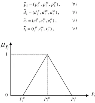
This work assumes the decision maker (DM) has already adopted the pattern of triangular possibility distribution for all imprecise coefficients. The possibility distribution can be stated as the degree of occurrence of an event with imprecise data. Figure 1 presents the triangular possibility distribution of imprecise number~p_i =(p_ip,p_im,p_io). In practice, a DM can construct the triangular possibility distribution ofp~i based on the following important values:

1. The most pessimistic value (p_ip) which has a very low likelihood of belonging to the set of available values (possibility degree = 0 if normalized).

2. The most possible value (p_im) that definitely belongs to the set of available values (possibility degree = 1 if normalized).

3. The most optimistic (p_io) that has a very high likelihood of belonging to the set of available values (possibility degree = 0 if normalized).

The imprecise data for the previous PLP model can thus be modeled with triangular possibility distributions, as follows:

) , , (

~ o

i m i p i

i p p p

p = , ∀i

) , , (

~ _o

i m i p i

i d d d

d = , ∀i

) , , (

~ o

i m i p i

i e e e

e = , ∀i

) , , (

~ o

i m i p i

i t t t

t = , ∀i

0 1

Pip Pim Pio

Figure 1. The triangular possibility distribution of pi

Pi

i P

μ

3.2. An auxiliary multiple objective linear programming (MOLP) model 3.2.1. Strategy for solving the imprecise objective function

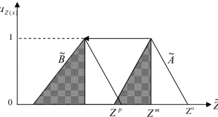
The imprecise objective function of the PLP model in the previous section has a triangular possibility distribution. Geometrically, this imprecise objective is fully defined by three prominent points (ZP,0), (Zm,1) and (Zo,0). The imprecise objective function can be minimized by pushing the three prominent points towards the left. Because the vertical coordinates of the prominent points are fixed at either 1 or 0, the three horizontal coordinates are the only considerations. Consequently, solving the imprecise objective requires minimizing Zp, Zm, and Zo simultaneously. Using Lai and Hwang’s (1992) approach, the approach developed here minimizes Zm, maximizes (Zm-Zp), and minimizes (Zo-Zm), rather than simultaneously minimizing Zp, Zm, and Zo. That is, the proposed approach simultaneously involves minimizing the most possible value of the imprecise total costs,

Zm_{, maximizing the possibility of obtaining a lower total costs, (Z}m_-Zp_{), and minimizing the risk of}

obtaining a higher total costs, (Zo-Zm). The last two objectives actually are relative measures from

Zm_{, the most possible value of the imprecise total costs.}

Figure 2 presents the strategy for minimizing the imprecise objective function.

As in Figure 2, we would prefer the possibility distribution ofB~to that ofA~. The following lists the result for the three new crisp objective functions of total earliness and tardiness costs in Eq. (1).

Figure 2. The strategy to minimize the total earliness and tardiness costs

∑

= + = = N i i m i i m i

m _{e E t T}

Z Z Min

1

1 ( ) (8)

∑

= − + − = − = N i i p i m i i p i m i p

m _{Z e e E t t T}

Z Z Max

1

2 ( ) (( ) ( ) ) (9)

∑

= − + − = − = N i i m i o i i m i o i m

o _{Z e e E t t T}

Z Z Min

1

3 ( ) (( ) ( ) ) (10)

3.2.2. Imprecise right hand side of constraints

As explained before, ~piand di

~

in equations (2) to (4) of the original PLP model, are imprecise and have the triangular possibility distribution. This work adopts the weighted average method proposed

Z

~

p

Z

_Z

m

) (x Z

μ

0 1

A

~

B

~

Zo

by Lai and Hwang (1992) to convert~p_iand d~_iinto crisp numbers. If the minimum acceptable possibility, λ, is given, then the auxiliary crisp constraints can be presented as follows:

) ( _{1 , 1 , 1 ,}

, 1 , 1 , 1 o i m i p i o i m i p i i i

i E X p p p d d d

T − − =φ _λ+φ _λ+φ _λ− φ _λ +φ _λ +φ _λ (11)

o i m i p i i ij

j MY X p p p

X + − ≥φ1 ,_λ+φ1 ,_λ+φ1 ,_λ (12)

o i m i p i j ij

i M Y X p p p

X + (1− )− ≥φ1 ,_λ+φ1 ,_λ +φ1 ,_λ (13)

where, φ₁+φ₂+φ₃ =1, and φ1,φ2,φ3denote the weights of the most pessimistic, most possible and

most optimistic values of the imprecise processing times and due dates. This work uses the most likely values concept of Lai and Hwang (1992), assuming φ2 =46andφ1 =φ3 =16. The reason for

using the most likely values here is that the most possible values usually are the most important ones and hence, to which more weights should be assigned.

3.3. Solving the auxiliary MOLP problem

The auxiliary MOLP problem in section 3.2 can be converted into an equivalent single-goal LP problem using the piecewise linear membership function of Hannan (1981), to represent the fuzzy goals of the DM in the MOLP model, together with the minimum operator of the fuzzy decision-making of Bellman and Zadeh (1970). First we should get the following Positive Ideal Solutions (PIS) and Negative Ideal Solutions (NIS) of the three objective functions (Hwang and Yoon, 1981 and Lai and Hwang, 1992):

Z1PIS= Min Zm , Z1NIS = Max Zm (14a)

Z2PIS=Max (Zm-Zp) , Z2NIS=Min (Zm-Zp) (14b)

Z3PIS=Min (Zo-Zm) , Z3NIS= Max (Zo-Zm) (14c)

The linear membership function of the three objective functions can be computed (see Figures 3, 4, and 5) as:

⎪ ⎪ ⎩ ⎪ ⎪ ⎨ ⎧ > ≤ ≤ − − < = NIS NIS PIS PIS NIS NIS PIS Z Z Z Z Z Z Z Z Z Z Z Z 1 1 1 1 1 1 1 1 1 1 1 0 1 1

μ (15)

⎪ ⎪ ⎩ ⎪ ⎪ ⎨ ⎧ < ≤ ≤ − − > = NIS NIS PIS NIS PIS NIS PIS Z Z Z Z Z Z Z Z Z Z Z Z 2 2 2 2 2 2 2 2 2 2 2 0 1 2

⎪ ⎪ ⎩ ⎪ ⎪ ⎨ ⎧ > ≤ ≤ − − < = NIS NIS PIS PIS NIS NIS PIS Z Z Z Z Z Z Z Z Z Z Z Z 3 3 3 3 3 3 3 3 3 3 3 0 1 3

μ (17)

Each linear membership function can be determined by asking the DM to specify the imprecise objective value interval. Figures 3, 4 and 5 are the graphs of linear membership functions for equations (15) to (17).

Figure 3.The membership functions ofZ1

Finally, using the fuzzy decision-making of Bellman and Zadeh (1970) and Zimmermann’s (1978) fuzzy programming method, we solve the following equivalent single objective linear programming model:

Max α (18)

s.t.

α

μ ≥

l

Z l=1,2,3 (19)

) (1 , 1 , 1 , , 1 , 1 , 1 o i m i p i o i m i p i i i

i E X p p p d d d

T − − =φ λ+φ λ+φ λ− φ λ+φ λ+φ λ (20)

o i m i p i i ij

j MY X p p p

X + − ≥φ1 ,_λ+φ1 ,_λ+φ1 ,_λ (21)

o i m i p i j ij

i M Y X p p p

X + (1− )− ≥φ1 ,_λ+φ1 ,_λ +φ1 ,_λ (22)

i i r

X ≥ , ∀i (23)

0 , , _{i i} ≥

i E X

T , ∀i (24)

1 , 0

= ij

Y , ∀i,j;i≠ j (25)

1

0≤α≤ ₍₂₆₎

PIS

Z

1 NIS

Z

1 1 Z

0

1

1 Z

μ

Figure 4. The membership functions ofZ2

The auxiliary variableα in the above model can be interpreted as representing the overall degree of DM’s satisfaction with the determined goal values.

Figure 5. The membership functions ofZ3 3.4. Solution algorithm

The algorithm of the proposed PLP approach to solve the single machine scheduling problem is as follows.

Step 1: Formulate the PLP model for the single machine scheduling problem.

Step 2: Model the imprecise coefficients (e~_i,~t_i) and the right-hand sides (p~_i,d~_i) using triangular possibility distributions.

Step 3: Develop three new crisp objective functions of the auxiliary MOLP problem that are equivalent to simultaneously minimizing the most possible total cost value, maximizing the possibility of obtaining lower costs, and minimizing the risk of obtaining higher costs.

Step 4: Given the minimum acceptable possibility, λ, convert the imprecise constraints into crisp

ones using the weighted average method or the fuzzy ranking concept. Here, we assign λ= 0.5.

Step 5: Specify the linear membership functions for three new objective functions, and then convert the auxiliary MOLP problem into an equivalent LP model using the fuzzy decisions of Bellman and Zadeh (1970) and Zimmermann’s (1978) fuzzy programming method. This paper considers the PIS of the three new objective functions as (Z1PIS, Z2

NIS

+0.5× Z2NIS, Z3PIS) and the NIS as (Z1PIS+0.5×

Z1PIS, Z2NIS, Z3PIS +0.5× Z3PIS ). 3

Z

μ

NIS

Z

₃ PIS

Z

3

3

Z

1

0

NIS

Z

2 2

Z

μ

0

1

PIS

Z

2

2

Step 6: Solve and modify the model interactively. If the DM is not satisfied with the initial solution, then the model must be modified until a satisfactory solution is found.

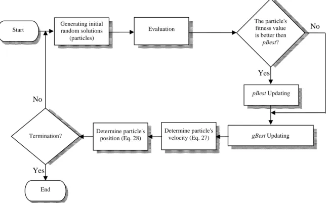
4. PARTICLE SWARM OPTIMIZATION

Particle swarm optimization (PSO) is a population based stochastic optimization technique that was developed by Kennedy and Eberhart (1995). The development of PSO was inspired by social behavior of bird flocking or fish schooling. In PSO, each solution is a bird in the flock and is referred to as a particle. A particle is analogous to a chromosome in GAs (Shi and Eberhart, 1998). All particles have fitness values which are evaluated by the fitness function to be optimized, and have velocities which direct the flying of the particles. The particles fly through the problem space by following the particles with the best solutions so far (Hu et al., 2004).

PSOs have been applied successfully to a wide variety of optimization problems to find optimal or near-optimal solutions. In real world, we need to determine the optimal or a near optimal sequence in scheduling problems, but solving the large size problems are hard and time consuming. Thus, in this paper, we apply the PSO to large size problems. The general scheme of the applied PSO is provided in Figure 6.

PSO is initialized with a group of random particles and then searches for optima by updating each generation. In every iteration, each particle is updated by following two best values. The first value is the location of the best solution a particle has achieved so far which is referred to as pBest. Another best value is the location of the best solution in all the population that has been achieved so

Yes Generating initial

random solutions (particles)

Evaluation

pBest Updating

No

gBest Updating Determine particle's

velocity (Eq. 27) Determine particle's

position (Eq. 28) Termination?

No

Yes End Start

The particle's fitness value is better then

pBest?

far. This value is called gBest (Hu et al., 2004). The particle swarm optimization algorithm is described in the following sections.

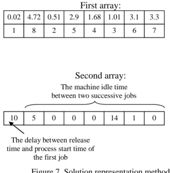
4.1. Solution representation

On one hand, the solution representation must have a one-to-one relation with the search space; on the other hand, the representation should be so that we are able to easily decode it to reduce the cost of the algorithm.

In this paper, we use a new continuous representation method. In this method we use two row arrays of the size equal to the number of the jobs to be scheduled. The first array shows the positions of jobs that are to be scheduled and the second array represents the machine idle times between two successive jobs. In the first array, the value of the first element of the array shows which job is scheduled first and the second value shows which job is scheduled second and so on.

Figure 7. Solution representation method

In this array the smallest value represents the first job; the second smallest value represents the second job and so on. In the second array, the value of the first element of the array indicates the time delay between release time and process start time of the first job and other values of this array represent the machine idle times between two successive jobs. Figure 7 illustrates an instance representation for 8 jobs.

4.2. Particle updating

The core of PSO which deals with updating the velocity and position of each particle can be represented by way of the following equations (Hu et al., 2004):

(27)

id id

id x V

x = + (28)

= id

V w.V_id +c₁.rand().(p_id −x_id)+ +

− )

().( .

2 Rand pgd xid c

First array:

1 8 2 5 4 3 6 7

0.02 4.72 0.51 2.9 1.68 1.01 3.1 3.3

Second array:

10 5 0 0 0 14 1 0

The delay between release time and process start time of

the first job

The machine idle time between two successive jobs

max

max V V

V ≤ id ≤

− (29)

Equation (27) calculates a new velocity for each particle based on its previous velocity (Vid), the

particle's location at which the best fitness so far has been achieved (p_id, or pBest), and the best location in the entire population (p_gd, or gBest) so far achieved. In this equation, Rand() and rand() are two random numbers generated independently in the range [0,1]. c1and c2are two learning

factors, which control the influence of pBest and gBest on the search process and w is an inertia weight which was first introduced by Shi and Eberhart (1998). The function of inertia weight is to balance the global exploration with the local exploitation and is proposed such that to decrease linearly with time from a value of 1.4 to 0.5 (Shi and Eberhart, 1998). Equation (28) updates each particle's position in the solution hyperspace. In equation (29) Vmaxis an upper limit on the

maximum change of particle velocity.

4. EXPERIMENTAL RESULTS

To verify and validate the proposed model, small and large-sized problems are randomly generated with respect to the parameter setting presented in Table 1. Using the branch-and-bound (B&B) method the small-sized test problems are optimally solved by the LINGO 8.0 software package. To solve large-sized instance problems, the particle swarm optimization algorithm has been coded in the Visual Basic 6 and executed on a Pentium 4, 3 GHz, 512 MB of RAM using Windows XP. The performance of the PSO was compared with the results from the LINGO 8.0 for small-sized instances. For both small and large-sized experiments, we consider the assumptions that follow.

General assumptions:

The due dates are uniformly distributed in the interval [P(1−τ−ρ₂),P(1−τ+ρ₂)]where

∑

=

= N

i m i P P

1 ,

andρ andτ are two parameters taking values 0.6, 0.2 respectively (Loukil et al., 2005). Whenτ increases, due dates become more restrictive; whenρincreases, due dates are more diversified.

Assumptions of PSO

In this paper, to tune the PSO, extensive experiments were conducted with different sets of parameters. At the end, the following set was found to be effective in terms of quality of solutions when compared against the Lingo results for small-sized problems. The parameters that need to be

Table 1. Model Parameters Setting Parameters value

Pip, Pim, Pio Pim-w1i U[10,100] Pim+w2i

w1i, w2i U[1, Pim]

dip, dim, dio dim-w3i U[P(1−τ−₂ρ),P(1−τ+ρ₂)] dim+w4i

w3i, w4i U[1, dim]

ri U[0,20]

eip, eim, eio U[1,4] U[4,8] U[8,12]

tuned are as follows: No of Generations (G), Population Size (Number of Particles) (N) and Learning factors (c1and c2) were set to 100, 50, 2.0, and 2.0, respectively. For each instance in

small and large-sized problems, we executed PSO 15 times.

For each small-sized problem, the results obtained were compared with the Lingo 8 results. The results for small and large-sized problems are displayed in Tables 2, 3, 4 and 5.

Table 2.Comparison of small-sized problems

No.

Jobs

* 1

Z *

2

Z *

3

Z Z~

Lingo PSO Lingo PSO Lingo

PSO Lingo

PSO

6

2165.3 2166.7 1748.1 1750.5 787.8 782.2 (417.2,2165.3,2953.1) (416.2,2166.7,2948.9)

7

2723.8 2767 2137.9 2169.8 1166.1 1178.8 (585.9,2723.8,3889.9) (597.2,2767,3945.8)

8

2987.6 2992 2042.1 2018.8 1127 1139.8 (945.5,2987.6,4114.6) (973.2,2992,4131.8)

9

3864.6 3990.7 2844.2 2938.6 1202.4 1200.9 (1020.4,3864.6,5067) (1052.1,3990.7,5191.6)

) , , ( ~

3 1 1 2

1 Z Z Z Z

Z

Z= − +

Table 3. Comparison of aspiration level values for small-sized problems

No.Jobs Lingo PSO − ×100

PSO PSO Lingo

α α α

6 0.6529 0.6514 0.0023027 7 0.7683 0.7326 0.0487305 8 0.7255 0.7132 0.0172462 9 0.3986 0.3755 0.0614731

Table 4. The PSO large-sized experimental results No.of

Jobs

Z1* Z2* Z3*

Ave STD Ave STD Ave STD

15 12981.2 520.5 9224.1 731 6440.5 294.3

20 18957.1 1226.8 13339.1 687.4 8648.8 570

50 173989.6 11429.5 115676.6 7300.2 95335.7 6264.2 80 441748.6 20426.7 296150.1 15055.2 289559 13231.5 100 733438.7 14482.9 494952.3 8933.9 478478.1 17934.8 200 3405205 147997.2 2242287 181973.1 2239673 56539.3

Table 5.The PSO large-sized aspiration level values No.of

Jobs

Z

~

α

_{CPU Time}

Ave Lingo PSO

15 (3757.1,12981.2,19421.7) * 0.6951 00:00:44 20 (5618,18957.1,27605.9) * 0.3688 00:00:56 50 (78653.9,173989.6,269325.3) * 0.5618 00:03:22 80 (145598.5,44174.6,731307.6) * 0.5792 00:09:59 100 (238486.4,733438.7,1211916.8) * 0.6161 00:11:20 200 (1162918,3405205,5644878) * 0.6772 00:38:20 * Lingo can not solve the problem

6. CONCLUSIONS

This work presents a novel PLP method for solving single machine scheduling problems with imprecise processing times, due dates, earliness and tardiness penalties, using triangular possibility distribution. The objective function is to minimize the total costs of earliness and tardiness. The applied method adopts the strategy of simultaneously minimizing the most possible value of the imprecise total costs, maximizing the possibility of obtaining a lower total cost, and minimizing the risk of obtaining a higher total cost. Some illustrative examples demonstrate the feasibility of applying the proposed approach to single machine scheduling problems. The PLP approach in this paper yields an efficient single machine scheduling with optimal solution and overall degree of DM satisfaction with determined goal values. Since the model is complicated, the conventional optimization methods cannot be utilized in reasonable time. Hence, an efficient meta-heuristic algorithm known as particle swarm optimization algorithm is used to solve the proposed model. REFERENCES

[1] Bellman R. E., Zadeh L. A. (1970), Decision-making in a fuzzy environment; Management Science 17; 141-164.

[2] Brucker P. (1998), Scheduling Algorithms; Springer, Berlin.

[3] Chanas S., Kasperski A. (2001), Minimizing maximum lateness in a single machine scheduling problem with fuzzy processing times and fuzzy due dates; Engineering Applications of Artificial Intelligence 14; 377-386.

[4] Chanas S., Kasperski A. (2003), On two single machine scheduling problems with fuzzy processing times and fuzzy due dates; European Journal of Operational Research 147; 281-296.

[5] Chang P. C. (1999), Branch and bound approach for single machine scheduling with earliness and tardiness penalties; Computers and Mathematics with Applications 37; 133-144.

[6] Chou F. D., Chang T. Y., Lee C. E. (2005), A heuristic algorithm to minimize total weighted tardiness on a single machine with release times; International Transactions in Operations Research 12; 215-233.

[7] Feldmann M., Biskup D. (2003), Single-machine scheduling for minimizing earliness and tardiness penalties by meta-heuristic approaches; Computers and Industrial Engineering 44; 307-323.

[8] Hannan E. L. (1981), Linear programming with multiple fuzzy goals; Fuzzy Sets and Systems 6; 235-248.

[9] Hu X., Shi Y., Eberhart R. (2004), Recent advances in particle swarm; in: Proceedings of 2004 Congress on Evolutionary Computation (CEC 2004), Portland, Oregon, Vol. 1, 90-97.

[10] Hwang C. L., Yoon K. (1981), Multiple attribute decision making: methods and applications; Springer

,

Berlin.

[11] Kennedy J., Eberhart R. (1995), Particle swarm optimization. Proceedings of the IEEE International Conference on Neural Networks (Perth, Australia), 1942–1948. Piscataway, NJ: IEEE Service Center. [12] Lam S. S., Cai X. (2002), Single machine scheduling with nonlinear lateness cost functions and fuzzy

[13] Lai Y. J., Hwang C. L. (1992), A new approach to some possibility linear programming problems; Fuzzy Sets and Systems 117; 35-45.

[14] Liaw C F (1999), A branch-and-bound algorithm for the single machine earliness and tardiness scheduling problem; Computers and Operations Research 26; 679-693.

[15] Lin S.W., Chou S.Y., Ying K.C. (2006), A sequential exchange approach for minimizing earliness-tardiness penalties of single-machine scheduling with a common due date; European Journal of Operational Research Article in Press.

[16] Loukil T., Teghem J., Tuyttens D. (2005), Solving multi-objective production scheduling problems using metaheuristics; European Journal of Operational Research 161; 42-61.

[17] Mazzini R., Armentano V. A. (2001), A heuristic for single machine scheduling with early and tardy costs; European Journal of Operational Research 128; 129-146.

[18] Mondal S. A., Sen A. K. (2001), Single machine weighted earliness/tardiness penalty problem with a common due date; Computers and Operations Research 28; 649-669.

[19] Peng J., Liu B. (2004), Parallel machine scheduling models with fuzzy processing times; Information Sciences 166; 49-66.

[20] Rabadia G., Mollaghasemi M., Anagnostopoulos G. C. (2004), A branch-and-bound algorithm for the early/tardy machine scheduling problem with a common due-date and sequence-dependent setup time; Computers and Operations Research 31; 1727-1751.

[21] Shi Y., Eberhart R. (1998), A modified particle swarm optimizer. Proceedings of the IEEE international conference on evolutionary computation. Piscataway, NJ: IEEE Press; 69–73.

[22] Tavakkoli-Moghaddam R.

,

Moslehi G., Vasei M., Azaron A. (2005), Optimal scheduling for a single machine to minimize the sum of maximum earliness and tardiness considering idle insert; Applied Mathematics and Computation 167; 1430-1450.

[23] Ventura J. A., Radhakrishnan S. (2003), Single machine scheduling with symmetric earliness and tardiness penalties; European Journal of Operational Research 144; 598-612.

[24] Wan G., Yen B. P. C. (2002), Tabu search for single machine scheduling with distinct due windows and weighted earliness/tardiness penalties; European Journal of Operational Research 142; 271-281. [25] Zimmermann H. J. (1978), Fuzzy programming and linear programming with several objective