Winter 2011
An Efficient Algorithm to Solve Utilization-based Model for Cellular
Manufacturing Systems
Kaveh Fallahalipour1, Iraj Mahdavi2, Ramin Shamsi3, Mohammad Mahdi Paydar4
1 MAPNA Turbine Engineering & Manufacturing Co. (TUGA), P.O.Box: 15875-5643, Tehran, Iran
2,4Department of Industrial Engineering, Mazandaran University of Science and Engineering, Babol, Iran 3
Department of Industrial and Management Systems Engineering, University of Nebraska-Lincoln, Lincoln, Nebraska, USA
[email protected] ABSTRACT
The design of cellular manufacturing system (CMS) involves many structural and operational issues. One of the important CMS design steps is the formation of part families and machine cells which is called cell formation. In this paper, we propose an efficient algorithm to solve a new mathematical model for cell formation in cellular manufacturing systems based on cell utilization concept. The proposed model is to minimize the number of voids in cells to achieve higher cell utilization. The proposed model is a non-linear model which cannot be optimally solved. Thus, a linearization approach is used and the linearized model is then solved by linear optimization software. Even after linearization, the large-sized problems are still difficult to solve, therefore, a Simulated Annealing method is developed. To verify the quality and efficiency of the SA algorithm, a number of test problems with different sizes are solved and the results are compared with solutions obtained by Lingo 8 in terms of objective function values and computational time.
Keywords: Cell formation, Mathematical model, Cell utilization, Simulated Annealing.
1. INTRODUCTION
Today’s markets enforce manufacturers to produce a wide variety of products with shorter product life cycles and small quantities. Under these situations, maintaining high efficiency in batch operations of traditional process-oriented manufacturing is very difficult. A relatively modern manufacturing approach which overcomes most of the usual problems of the traditional production systems is Group Technology (GT). GT is a manufacturing philosophy that organizes and uses information for grouping various parts and products with similar machining requirements into families of parts and corresponding machines into machine cells (Hyer and Wemmerlov 1984). One specific application of GT is cellular manufacturing system (CMS) which is a production approach aimed at increasing efficiency and flexibility by utilizing the process similarities of the parts. It
Corresponding Author
involves grouping similar parts into part families and the corresponding machines into machine cells. The main advantages of CMS have been reported in the literature as reduction in setup time, reduction in throughput time, reduction in work-in-process inventories, reduction in material handling costs, better quality and production control, increment in flexibility, etc. (Wemmerlov and Hyer 1989, Heragu 1994 and Wemmerlov and Johnson 1997). The cell formation (CF) is one of the key issues in the design of CMS. In the past several years, many solution approaches have been developed for solving CF. Researchers have mainly used zero–one machine- part incidence matrix as the input data for the problem. A detailed review of the pervious researches and solution methods for CF can be found in Singh (1993), Joines et al (1996), Selim et al (1998), Yin and Yasuda (2006), and Papaioannou and Wilson (2010).
Hyer (1984) collected data on 20 U.S. firms through a detailed questionnaire to gather information on the costs and benefits of CM. A large majority of the respondents reported that the actual benefits from implementing CM met or exceeded their expectations. Specific savings generally occurred in reductions of lead times, throughput times, queuing times, setup times, work-in-process, labor costs, material handling costs, and in easier process plan preparation. Collet and Spicer (1995) in a case analysis of a small manufacturing company found that cellular manufacturing resulted in a number of performance improvements when compared to job shops. Operating time was reduced and less work space due to the less work-in-process were the results of CMS in addition to the reduction in setup cost.
As mentioned above, CF identifies the machine cells and part families which is a key step in designing a CMS. At the conceptual level, CF models ignore many manufacturing factors and only consider the machining operations of the products, so that a manufacturing system is represented by a binary machine-part incidence matrix A=[aij], which is a zero-one matrix of order
P M
where Pis the number of products and M is the number of machines. If aij=1, it means that part i requires processing on machine j, otherwise aij= 0.
Mathematical programming is widely used for modeling CMS problem by different objective functions in the literature. Kusiak (1987) suggested the p-median model for group technology to minimize the total sum of distances between each product/machine pair. Adil et al. (1993) proposed an assignment allocation algorithm, a non-linear mathematical model, to identify part families and machine groups simultaneously without manual intervention. The objective of the method is to explicitly minimize the weighted sum of the exceptional elements and voids. Ronald (1997) presented 0-1 integer programming to form minimum-cost machine cells with exceptional parts. Albadawi et al. (2005) proposed a mathematical approach for forming manufacturing cells. The proposed approach involves two phases. In the first phase, machine cells are identified by applying similarity coefficients. In the next phase, an integer-programming model is presented to allocate parts to the identified machine cells. Mahdavi et al. (2007) presented a mathematical model for CF in cellular manufacturing based on cell utilization concept for minimizing the number of voids in cells to achieve the higher performance of cell utilization.
Currently, metaheuristics have been mainly developed for the solution of NP-hard problems. The CF problem is considered to be a complex and difficult optimization problem. To gain more benefits of CMS, many researchers have applied metaheuristic algorithms. The most notable metaheuristics applied to CF are: genetic algorithms (Onwubolu and Mutingi 2001, Goncalves and Resende 2004), simulated annealing (Sofianopoulou 1997 and Wu et al. 2008), neural networks (Majeed Ali and Vrat 1999 and Soleymanpour et al. 2002) and tabu search (Lozano et al. 1999 and Wu et al. 2004).
Chen and Cheng (1995) considered a neural network-based cell formation algorithm in cellular manufacturing. They used an adaptive resonance theory (ART) based neural network to the CF. The main advantage of using an ART network is fast computation and the outstanding ability to handle large scale industrial problems. Mahdavi et al. (2001) presented a graph-neural network manufacturing approach for cell formation. Their research has the ability to handle large scale problems. Onwubolu and Muting (2001) developed a genetic algorithm, which accounts for inter-cellular movements and the cell-load variation. Soleymanpour et al. (2002) applied a transiently chaotic neural network approach (TCNN) to solving a mathematical model in design of CM. The approach adopted for the simultaneous grouping of similar parts and machines is based on minimizing the total number of exceptional elements and voids. Goncalves and Resende (2004) presented a hybrid algorithm combining a local search and a genetic algorithm with very promising results. Wu et al. (2008) proposed a simple effective simulated annealing-based approach for CF problem when the manufacturing system is represented by a 0-1 machine-part incidence matrix. Megala et al. (2008) considered the problem of cell-formation in cellular manufacturing systems with the objective of maximizing the grouping efficacy. They proposed an Ant-Colony Optimization (ACO) algorithm to obtain machine-cells and part-families. Fallahalipour and Shamsi (2008) introduced a mathematical model for CF in CMS using sequence data with the goal of minimizing total costs of inter and intra-cell movements and utilization concept. Safaei et al. (2008) used an efficient hybrid meta-heuristic based on mean field annealing (MFA) and simulated annealing so-called MFA-SA to solve an extended model of dynamic cellular manufacturing system problem, the way they analyzed the quality of the solutions is widely used in section 5 of this paper. The rest of this paper is organized as follows: in Section 2 the problem formulation of the proposed model is presented. A numerical example is described in section 3. Implementation of SA and the computational results are described in Section 4. Finally, conclusion is given in Section 5.
2. MATHEMATICAL MODEL
In this section, we formulate the new mathematical model based on machine-part relationship in CMS. The proposed model deals with the minimization of the number of voids in cells for better cell utilization.
Indexing sets
i index for parts (i =1, 2,…, P)
j index for machines (j =1, 2… M)
k index for cells (k =1, 2,…, C) Parameters
Lk: lower bound of the number of machines in cell k.
Uk: upper bound of the number of machines in cell k.
LP: lower bound of the number of parts in cells. Min_utk: minimum utilization for cell k.
M: large positive value
1 if part nedd to machine ,
0 otherwise.
ij
i
j
r
Decision variable
1 if machine is assigned to cell ,
0 otherwise.
jk
j
k
Y
1 if part is assigned to cell ,
0 otherwise.
ik
i
k
Z
Objective function
We formulate the objective function as:
1 1 1 1 1
Z =
-C P M P M
ik jk ik jk ij
k i j i j
Min
Z Y
Z Y
r
(1)The objective function accounts for calculation of total number of voids in all cells.
Constraints
Lower and upper bound for the number of machines to be allocated to cells:
1
M
Y jk Lk k
j
(2) 1 MY jk Uk j
k (3)Each machine must be allocated to one cell:
1
1
C jk kY
j (4) Each part must be assigned to one cell:1
1
C ik kZ
i (5) Lower limit of number of parts in each cell:1 P ik i
Z
LP
We could specify minimum utilization of cells to be achieved as follows:
k
1 1 1 1
_ut
P M P M
ik jk ij ik jk
i j i j
z y r
Min
z y
k (7) Constraint (5) ensures that each part is assigned to only one cell. Also, this assignment is according to maximum number of operations of that part to be performed in that cell. The constraints (8), (9) and (10) guarantee that each part type can be assigned to cells containing maximum number of operations of that part. These constraints help in reducing the number of exceptional elements.
M
j ij jk
m i k y r
f
1
, i k, (8)
(
,
)
max
i
Max
f
i
k
f
mk
i (9)
max
1
1
( , )
ik m
Z
f
i
f
i k
M
i k, (10)
0
,
1
,
jk
ikY
Z
i j k, , (11) Linearization of the mathematical modelIt is obvious that Eqs. (1) and (7) are nonlinear functions. These functions can be linearized by defining new binary variable Wijk, which is computed by the following equation:
ijk ik jk
W
Z Y
The following equations should be added to the original proposed model:
1.5 0
ijk ik jkW
Z
Y
i j k, , (12)1.5
W
ijk
Z
ik
Y
jk
0
i j k, , (13) 3. A NUMERICAL EXAMPLE
This section aims to verify the applicability of the proposed model, so an example from the literature is chosen (Singh and Rajamani, 1996). Table 1 shows the machine-part incidence matrix
Table1 5 x 7 machines - part matrix; Singh and Rajamani (1996) i
j 1 2 3 4 5 6 7
1 0 1 0 1 0 0 1
2 0 0 1 0 1 0 0
3 1 1 0 1 0 0 1
4 1 0 1 0 0 1 0
to the example which includes 5 machines and 7 parts. This example is solved by branch-and-bound (B&B) method under Lingo 8.0 software on an Intel® Celeron® 3.01 GHz Personal Computer with 1024 Mb RAM. This example is generated according to the information provided Table 2.
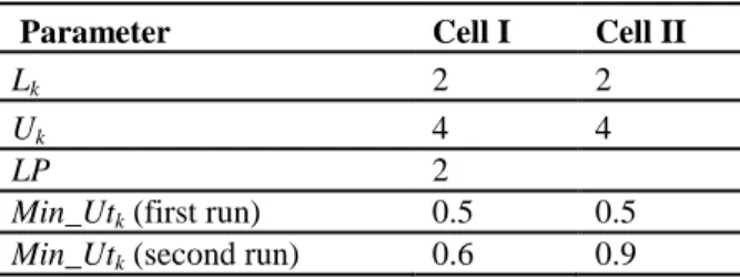
Table 2 Parameter setting for typical problem
Parameter Cell I Cell II
Lk 2 2
Uk 4 4
LP 2
Min_Utk (first run) 0.5 0.5
Min_Utk (second run) 0.6 0.9
After linearization, the proposed model includes 115 variables and 203 constraints and its computation time is 2 second. This example was run twice in which the minimum cell utilization of the first and the second run is assumed (0.5, 0.5) and (0.9,0.6) respectively. The optimum solution (Zbest) was found after two seconds in both runs. The cell configurations corresponding to the best obtained solution are shown in Figure 1.
C1 C2
M1 M3 M2 M4 M5
C1
P1 1 1
P2 1 1
P4 1 1 1
P7 1 1 C2
P3 1 1 1
P5 1 1
P6 1 1
C1 C2
M1 M3 M2 M4 M5 C1
P2 1 1
P4 1 1 1
P7 1 1
C2
P1 1 1
P3 1 1 1
P5 1 1
P6 1 1
Utilization cell I= 0.5, Utilization cell II=0.5 Utilization cell I= 0.9, Utilization cell II=0.6 Figure 1 Best obtained cell configurations for typical test problem
4. THE PROPOSED ALGORITHM
The proposed model falls in a class of NP-Hard problems. Therefore, determination of a final optimum solution under these conditions and constraints becomes difficult or even impossible for large practical problems in reasonable amount of computational time. In this paper, SA algorithm has been used and designed to solve the proposed model.
4.1. Simulated annealing implementation
Simulated annealing is a local search algorithm (Metaheuristic) introduced by Kirkpatrick et al. (1983) as a method to solve combinatorial optimization problems. Easy implementation, convergence properties and use of hill-climbing moves to escape local optima have made it a popular technique over the past two decades. The key algorithmic feature of simulated annealing is that it provides a means to escape local optima by allowing hill-climbing moves (i.e., moves which worsen the objective function value). SA begins with an initial solution (init_sol) and an initial temperature (T), cooling rate β and an iteration number (E1).
The possibility of the acceptance of a deteriorating solution is controlled by Temperature (T), and an iteration number (E1) is in charge of the number of repetitions until a stable state under the
necessary temperature. Temperature provides a means of flexibility while at high temperatures (early in the search), there is some flexibility to the situation to deteriorate; but at lower temperatures (later in the search) less flexibility exists.
A new neighborhood solution (Φ′) is generated based on T and E1 through a heuristic perturbation on the existing solutions. The neighborhood solution (Φ′) becomes the current solution (Φ) if the changes of the objective function (ΔTC=TC (Φ′) −TC (Φ)) is improved (i.e. TC (Φ′)≤TC (Φ)). Even though it is not improved, the neighborhood solution becomes a new solution with an appropriate probability based on
TC T e
.
This reduces the possibility of entrapment in a local optimum. The algorithm terminates upon reaching a predetermined number of iteration, K, or if there is no improvement in the objective function after repetition.
4.1.1. Solution representation
In the proposed algorithm, we have developed two matrixes for each solution representation. The first, namely Machine-Cell, shows machines assignment to the cells and it is a C×Uk array matrix, for an example of a 6×6×2 problem with Uk=4; which means there are 2 cells, 6 parts and 6 machines. Figure 2 represents Machine-Cell matrix.
2
5
6
0
1
3
4
0
Figure 2 Machine-Cell matrix of a solution
Figure 2 shows that machines 2, 5 and 6 are assigned to cell I and machines 1, 3 and 4 are assigned to cell II.
The second matrix, namely Part-Cell, displays assignment of the parts to cells and it is a C×H, where H = P-C×LP+LP. For a problem of size 6×6×2 with LP = 2, a typical Part-Cell matrix is shown in Figure 3.
2
6
0
0
1
3
4
5
Figure 3 Part-Cell matrix of a solution 4.1.2. Proposed SA algorithm
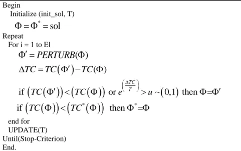
In this paper, a meta-heuristic algorithm based on simulated annealing (SA) is proposed. The pseudo code of this algorithm is illustrated in Figure 4. The main steps of the proposed SA are as follows:
Step 1. Initial solution generation
The initial solution is randomly generated. For this purpose, as mentioned in Section 4.1.1, we used two matrixes to represent a solution. At first, a machine is selected randomly and then assigned to a
cell until Lk is met, after that for remained machines, a randomly selected cell will be used to assign machines considering Uk.
The generated Machine-Cell matrix will construct the Part-Cell matrix based on maximum number of operations in each cell, so generation of infeasible solutions is possible because of lower bound on the number of parts in cells. If so, this step will be repeated. In addition, initial temperature, T0, epoch length, E1, the number of generated solutions in each temperature, maximum number of iterations, K, and cooling rate, β, are initialized in this step. Then, the objective function of the initial solution will be calculated.
Step 2. Temperature updating
The temperature is decreased according to the following equation: Ti+1 = β × Ti where, β is the cooling rate and is equal to 0.9 or 0.88. If the number of iterations is not less than Maximum Number of Iteration, K, go to step 3, otherwise go to step 6, set counter = 1.
Step 3. Neighborhood generation
In order to obtain the neighborhood solution from the current solution, a cell is randomly chosen from the cells which have more than Lk machines. A machine of that cell is selected randomly too and the algorithm transfers that machine to another cell where it does not make the solution infeasible.
Begin
Initialize (init_sol, T)
*sol
RepeatFor i = 1 to El
PERTURB
( )
TC
TC
TC
( )
if
or
0,1 then =
TC T
TC
TC
e
u
if
TC
TC
*
then
*=
end forUPDATE(T) Until(Stop-Criterion) End.
Figure 4 Proposed SA pseudo-code Step 4. Acceptance criteria
In this step, we decide to whether replace the current solution with the neighborhood solution or not. The current solution will be replaced with the neighborhood solution if its corresponding O.F.V. (TC (Φ′)) is less than or equal to the O.F.V of the current solution (TC (Φ)). Even if the neighborhood solution is not better than the current solution, in order to allow the algorithm to leave a local optimum, the neighborhood solution will be accepted if the Metropolis Condition is met.
According to Metropolis condition, a worse solution will be accepted as the current solution with the probability of
( )
iTC T r
P A
e
where ΔTC=TC (Φ′) −TC (Φ).Step 5. Counter updating
The counter counts the maximum number of solutions generated in each temperature. In this step, it is decided whether we have reached the maximum number of solutions in each iteration or not. If this maximum is not reached (i.e. counter < E1) go to step 4, otherwise, go to step 2.
Step 6. Termination
The algorithm will be terminated if the number of iterations is reached a predetermined number (M). To prevent losing an optimal solution, the best solution found so far (Φ*) is kept. A better solution generated from the current solution will be compared with Φ* and if it is better than Φ*,
Φ* will be replaced by it. In the initializing step, Φ* is initialized and will be the same as the random initial solution.
5. COMPUTATIONAL RESULTS
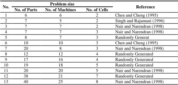
To verify the performance of the SA approach, we solved 13 problems from the literature (9 small/medium-sized + 4 large-sized) as given in Table 3.
Table 3 Source of problems
No. Problem size Reference
No. of Parts No. of Machines No. of Cells
1 6 6 2 Chen and Cheng (1995)
2 7 5 2 Singh and Rajamani (1996)
3 7 7 2 Nair and Narendran (1998)
4 7 7 3 Nair and Narendran (1998)
5 8 7 3 Randomly Generat
6 10 10 3 Chen and Cheng (1995)
7 20 8 3 Nair and Narendran (1998)
8 12 12 4 Randomly Generated
9 17 16 4 Randomly Generated
10 19 18 5 Randomly Generated
11 20 20 5 Nair and Narendran (1998)
12 38 21 7 Randomly Generated
13 40 25 8 Nair and Narendran (1998)
We consider a time criterion to determine the number of solved instances. For small/medium-sized problems, we started from a small-sized problem and increased gradually the size of the problem by a specific rule until the exact approach could not reach the feasible space within a predetermined run time. In a similar fashion, for large sized problems, we started from the largest medium-sized problems and increased the size of problem by a specific rule until the heuristic approach could not reach the feasible space within a predetermined run time (Safaei et al. 2008).
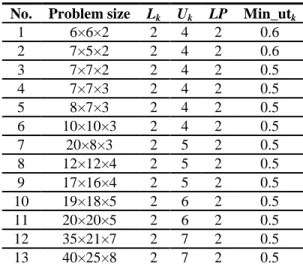
Some problems are generated randomly based on similar data in the literature. The problem sizes and other related information are shown in Table 4.
Table 4 Parameter setting of the problems No. Problem size Lk Uk LP Min_utk
1 6×6×2 2 4 2 0.6
2 7×5×2 2 4 2 0.6
3 7×7×2 2 4 2 0.5
4 7×7×3 2 4 2 0.5
5 8×7×3 2 4 2 0.5
6 10×10×3 2 4 2 0.5
7 20×8×3 2 5 2 0.5
8 12×12×4 2 5 2 0.5
9 17×16×4 2 5 2 0.5
10 19×18×5 2 6 2 0.5
11 20×20×5 2 6 2 0.5
12 35×21×7 2 7 2 0.5
13 40×25×8 2 7 2 0.5
The computation of each problem is allowed for 10000 seconds (2.7 hours). The optimal solution for the proposed model cannot be reached in 10000 seconds or even longer for medium and large-sized examples because of its complexity nature. Thus, to solve the small and medium-large-sized problems, we considered a possible interval for optimum value of objective function (F*) constructed by the Fboundand Fbest values. These values are introduced by Lingo software whereFbound F*Fbest.
According to the Lingo, Fbest indicates the best feasible objective function value (OFV) found so far. Fboundindicates the bound on the objective function values.
A limit on how far the solver will be able to improve the objective is this bound. At some point, these two values may become very close. These two values are close indicates that Lingo’s current best solution is either the optimal solution or very closes to it because of the fact that best objective value can never surpass the bound.
When such a point is available, the user may interrupt the solver and use the current best solution in order to save additional computation time. As mentioned earlier, we interrupt the solver when the computation time reached 10000 seconds. The SA parameter setting is shown in Table 5.
Table 5 SA parameter setting
No. 1 2 3 4 5 6 7 8 9 10 11 12 13
T0 10 10 10 10 10 10 10 12 25 25 28 30 32
El 4 4 5 5 6 11 17 15 28 35 41 80 100
K 100 100 100 100 100 100 100 100 100 100 100 100 100 β 0.9 0.9 0.9 0.9 0.9 0.88 0.88 0.88 0.88 0.88 0.88 0.88 0.88
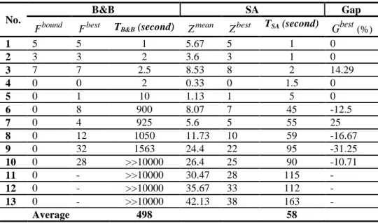
Comparison between the results obtained by B&B and SA are presented in Table 6 for 13 small/medium and large-sized problems. Each problem was run 15 times and the mean of OFV (
mean
Z ), best OFV (Zbest), and also the mean of CPU time (TSA) is reported in Table 6. The relative gaps between the best OFV found by B&B (Fbest) and Zmean found by SA are shown in
column ‘‘
G
mean’’. TheG
mean is calculated as: Gmean ZmeanFbest Fbest100. Also, the relative gaps between Fbest and Zbest are shown in column ‘‘G
best’’. In a similar manner, TheG
best is calculated as: Gbest ZbestFbest Fbest100Table 6 Comparison between B&B and SA runs for small and large-sized problems No.
B&B SA Gap
bound
F Fbest TB&B (second) Zmean Zbest TSA (second) Gbest(%)
1 5 5 1 5.67 5 1 0
2 3 3 2 3.6 3 1 0
3 7 7 2.5 8.53 8 2 14.29
4 0 0 2 0.33 0 1.5 0
5 0 1 10 1.13 1 5 0
6 0 8 900 8.07 7 45 -12.5
7 0 4 925 5.6 5 55 25
8 0 12 1050 11.73 10 59 -16.67
9 0 32 1563 24.4 22 95 -31.25
10 0 28 >>10000 26.4 25 90 -10.71
11 0 - >>10000 30.47 28 115 -
12 0 - >>10000 35.67 33 112 -
13 0 - >>10000 42.13 38 163 -
Average 498 58
Table 7 Comparison between three criteria for small and large-sized problems No.
Gap
mean
G (%) Gbest(%) (%)
1 13.4 0 13.4
2 20 0 20
3 21.58 14.29 7.56
4 0 0 0
5 13 0 13
6 0.875 -12.5 13.37
7 40 25 15
8 -2.25 -16.67 14.42
9 -23.75 -31.25 7.5
10 -5.71 -10.71 4.99
11 - - -
12 - - -
13 - - -
Ave. 7.74 -3.18 10.92
To evaluate the performance, ‘‘
G
mean’’ andG
best, Fbest are used as measures.Thus, a negative value indicates a better performance. Table 7 shows the comparison between the results obtained from B&B and the SA algorithm for the 13 small and large-sized problems considered in Table 6. The columns of Table 7 show the values ofG
meanandG
best resulted from SA. In general, thesmaller values of
G
mean,G
best andave G
mean
G
best
are more favorable and indicates higher quality of the solution.Obviously, the measure
ave G
mean
G
best
directly depends on the standard deviation of OFV in the 13 runs. As shown in the last row of Table 7, the average values ofG
mean,G
best and
mean best
ave G
G
resulted from SA are 7.74%, -3.18% and 10.95%, respectively. In other words, Zmean is 7.74% worse, in average, than Fbest while Zbest is 3.18% better, in average, than Fbest .Figure 5 Comparison between B&B and SA results (Table 5): (Zbestfound by SA) vs. (Fboundand Fbest).
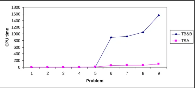
Figure 6 Comparison between CPU times related to the SA and B&B 0
5 10 15 20 25 30 35
1 2 3 4 5 6 7 8 9 10
O
F
V
problem
Zbest Fbound Fbest
0 200 400 600 800 1000 1200 1400 1600 1800
1 2 3 4 5 6 7 8 9
Problem
C
P
U
t
im
e
TB&B TSA
There is also an average of 10.95% difference between Zmean and Zbest. The average of CPU time is 29 seconds that is a promising result in comparison to the CPU time reported for B&B. Figures 5 and 6 show the behavior of Zmean and Zbest values obtained by SA versus Fbest and
bound
F according to the information shown in Table 6. In these figures, the problems are arranged in terms of Fbestvalues. The obtained results show that the SA is a suitable approach to solve the small and large-sized problems.
6. CONCLUSION
In this paper a new optimization model of cell formation based on cell utilization concept in cellular manufacturing systems (CMS) is introduced. The proposed model determines the cell configuration based on cell utilization concept with the aim of minimizing the number of voids in cells. We solved typical example problems for different values of cell utilization and showed how cell utilization can affect the cell configuration. An efficient algorithm based on simulated annealing (SA) was designed to solve the mathematical model. In order to verify the performance of the SA approach, we solved 13 benchmark problems (9 small/medium-sized +4 large-sized). The performance of SA was evaluated and compared to the performance of the branch-and-bound (B&B) method with respect to some defined measures. We observed that SA is an effective and efficient method in solving these CMS problems as the results are very promising.
REFERENCES
[1] Adil G. K., Ragamani D., Strong D. (1993), A mathematical model for cell formation considering investment and operational costs; European Journal of Operational Research 69; 330–341.
[2] Albadawi Z., Bashir H.A., Chen M. (2005), A mathematical approach for the formation of manufacturing cells; Computers & Industrial Engineering 48; 3–21.
[3] Chen S.J., Cheng C.S. (1995), A neural network based cell formation algorithm in cellular manufacturing; International Journal of Production Research 33(2); 293- 318.
[4] Collet S., Spicer R. (1995), Improving productivity through cellular manufacturing; Production and Inventory Management Journal 36(1); 71–75.
[5] Fallahalipour K., Shamsi R., A mathematical model for cell formation in CMS using sequence data (2008); Journal of Industrial and Systems Engineering 2(2); 144-153.
[6] Goncalves J., Resende M. (2004), An evolutionary algorithm for manufacturing cell formation; Computers & Industrial Engineering 47; 247–273.
[7] Heragu S.S. (1994), Group technology and cellular manufacturing; IEEE Transactions on Systems, Man and Cybernetics 24(2); 203–214.
[8] Hyer N. (1984), The Potential of Group Technology for U.S. Manufacturing; Journal of Operations Management 4(3); 183-202.
[9] Hyer N., Wemmerlov U. (1984), Group technology and productivity; Harvard Business Review, July-August; 140-149.
[10] Joines J.A., King R.E., Culbreth C.T. (1996), A comprehensive review of production oriented manufacturing cell formation techniques; International Journal of Flexible Automation and Integrated Manufacturing 3; 225–265.
[11] Kirkpatrick S., Gelatt C. D., Vecchi M. P. (1983), Optimization by simulated annealing; Science 220; 671-680.
[12] Kusiak A. (1987), The generalized group technology concept; International Journal of Production Research 25(4); 561–569.
[13] Lozano S., Adenso-Diaz B., Eguia I., Onieva L. (1999), A one-step tabu search algorithm for manufacturing cell design; Journal of the Operational Research Society 50; 509–16.
[14] Majeed Ali A. A., Vrat P. (1999), Manufacturing cell formation: a neural network approach; Proceedings of the International Conference on Operations Management for Global Economy Challenges and Prospects; Indian Institute of Technology, New Delhi, India, 565-571.
[15] Mahdavi I., Kaushal O.P., Chandra M. (2001), Graph-neural network approach in cellular manufacturing on the basis of a binary system; International Journal of Production Research 39(13); 2913–2922.
[16] Mahdavi I., Javadi B., Fallah-Alipour K., Slomp J. (2007), Designing a new mathematical model for cellular manufacturing system based on cell utilization; Applied Mathematics and Computation 190; 662–670.
[17] Megala N., Rajendran C., Gopalan R. (2008), An ant colony algorithm for cell-formation in cellular manufacturing systems; European Journal of Industrial Engineering 2(3); 298-336.
[18] Nair G.J., Narendran T.T. (1998), CASE: A clustering algorithm for cell formation with sequence data; International Journal of Production Research 36; 157–179.
[19] Onwubolu G.C., Mutingi M. (2001), A genetic algorithm approach to cellular manufacturing systems; Computers & Industrial Engineering 39, 125–44.
[20] Papaioannou G., Wilson J.M. (2010), The evolution of cell formation problem methodologies based on recent studies (1997–2008): Review and directions for future research; European Journal of Operational Research 206(3); 509-521.
[21] Ronald B.H. (1997), Forming minimum-cost machine cells with exceptional parts using zero-one integer programming; Journal of Manufacturing Systems 16(2); 79-90.
[22] Safaei N., Saidi-Mehrabad M., Jabal-Ameli M.S. (2008), A hybrid simulated annealing for solving an extended model of dynamic cellular manufacturing system; European Journal of Operation Research 185; 563–592.
[23] Selim H.M., Askin R.G., Vakharia A.J. (1998), Cell formation in group technology: review, evaluation and directions for future research; Computers and Industrial Engineering 34; 3–20.
[24] Singh N. (1993), Design of cellular manufacturing systems: an invited review; European Journal of Operational Research 69; 284–291.
[25] Singh N., Rajamani D. (1996), Cellular manufacturing systems design, planning and control; Chapman and Hall Publishing; London, UK.
[26] Sofianopoulou S. (1997), Application of simulated annealing to a linear model for the formation of machine cells in group technology; International Journal of Production Research 35, 501–511. [27] Soleymanpour M., Vrat P., Shanker R. (2002), A transiently chaotic neural network approach to the
design of cellular manufacturing; International Journal of Production Research 40(10), 2225-2244. [28] Wemmerlov U., Hyer N.L. (1989), Cellular manufacturing in the US industry: a survey of users;
International Journal of Production Research 27(9); 1511–1530.
[29] Wemmerlov U., Johnson D.J. (1997), Cellular manufacturing at 46 user plants: implementation experiences and performance improvements; International Journal of Production Research 35(1); 29– 49.
[30] Wu T., Low C., Wu W. (2004), A tabu search approach to the cell formation problem; International Journal ofAdvanced Manufacturing Technology 23; 916–924.
[31] Wu T.H., Chang C.C., Chung S.H. (2008), A simulated annealing algorithm for manufacturing cell formation problems; Expert Systems with Applications 34; 1609–1617.
[32] Yin Y., Yasuda K. (2006), Similarity coefficient methods applied to the cell formation problem: A taxonomy and review; International Journal of Production Economics 101; 329-352.