New High Accuracy Non-polynomial Spline Group Explicit Iterative Method for Two Dimensional Elliptic Boundary Value Problems

(1)

Sharif University of Technology

Scientia Iranica

Transactions D: Computer Science & Engineering and Electrical Engineering www.scientiairanica.com

New high-accuracy non-polynomial spline group

explicit iterative method for two-dimensional elliptic

boundary value problems

J. Goh

_{and N.H.M. Ali}

School of Mathematical Sciences, Universiti Sains Malaysia, 11800 Pulau Pinang, Malaysia. Received 9 September 2015; received in revised form 24 May 2016; accepted 20 August 2016

KEYWORDS Non-polynomial spline;

Finite dierence method; Group explicit iterative method; Elliptic partial dierential equation.

Abstract. In this paper, we propose a new high-accuracy method based on non-polynomial spline for the numerical solution to two-dimensional elliptic partial dierential equations. Using a non-polynomial spline approximation in x-direction and central dierence in y-direction, we obtain a new nine-point compact nite-dierence formulation. A four-point Group Explicit (GE) iterative scheme with an acceleration tool is then applied to the obtained system. The formulation procedure is presented in detail. The eciency of the proposed method is then illustrated by some test problems. The numerical results are found to be in good agreement with the exact solutions.

1. Introduction

Equilibrium problems in two or higher dimensions often lead to the elliptic partial dierential equations. These equations arise very frequently in describing velocity potentials, stationary distribution of temperatures, po-tential ows, and structural mechanics. Thus, solving this type of equation has been of interest to many researchers [1-5]. We consider the two-dimensional elliptic partial dierential equation of the form:

@2_u

@x2+

@2_u

@y2=A(x; y)

@u

@x+B(x; y) @u

@y+g(x; y);

(x; y) 2 ; (1)

dened in solution domain = f(x; y) : 0 < x; y < 1g with boundary @, where A(x; y) > 0 and B(x; y) > 0 *. Corresponding author. Tel.: +604 653 3924;

E-mail address: [email protected] (J. Goh) doi: 10.24200/sci.2017.4487

in . The corresponding Dirichlet boundary conditions are prescribed by:

u(x; y) = (x; y); (x; y) 2 @: (2)

Assume that the boundary conditions are given with sucient smoothness to maintain the order of accuracy in the numerical method under consideration.

The construction of group iterative methods in solving the elliptic partial dierential equation with promising results and improved execution timings has been greatly observed since the 1980s [6-12]. The methods were formulated using a combination of skewed nite-dierence approximations together with the centred-dierence approximation that resulted in schemes with better rates of convergence than the exist-ing iterative methods available in literature. However, one of the weaknesses of these formulations is that the formulas are based purely on nite-dierence dis-cretization which enables the solutions to be obtained only at certain intersection points of the grid lines in the solution domain.

The application of splines to solving dierential equations has been an active area of research over the

(2)

last few decades. In 1968, Bickley [13] originated an idea to obtain better accuracy for a linear ordinary dierential equation by using cubic splines method. Following this, Albasiny and Hoskins [14] applied the cubic spline interpolation to solve a two-point bound-ary value problem. At about the same time, Fyfe [15] examined the method suggested by Bickley [13] and carried out the error analysis. Fyfe concluded that spline method is better than the usual nite-dierence method as the spline method has the exibility to get the solution at any point in the domain with more ac-curate results. Due to its simplicity, many researchers started considering spline as one of the approximation tool to obtain accurate numerical solutions [16-19]. Recently, Ding et al. [20] and Gopal et al. [21] have studied non-polynomial spline methods for the numer-ical solution to one-dimensional hyperbolic problem. More recently, Jha and Mohanty [22] have formulated the solution to nonlinear second-order boundary value problems by using quintic non-polynomial spline. To the best of the authors' knowledge, no high-accuracy non-polynomial spline method has been investigated on two-dimensional elliptic partial dierential equations. Since the spline method has the exibility to produce approximations at any point in the domain with high-accuracy solutions, there has been an interest to for-mulate group iterative schemes in hybrid with splines in solving the elliptic partial dierential equations. Goh and Ali [23] managed to derive a new method, namely the Spline Explicit Group (SEG) iterative method, which incorporates cubic spline with group iterative scheme for solving the elliptic equation with the promising results. However, with the emergence of newer types of splines with more favorable properties, it would be a worthwhile eort to investigate the application of highly advanced types of splines to the group schemes as a means to further improve the performance of the methods.

In this paper, we aim to discuss the formulation of a new numerical method which incorporates a non-polynomial spline into combination with a group explicit iterative scheme for solving a two-dimensional elliptic partial dierential equation. We will present the proposed method as follows. In the next section, we discuss the non-polynomial spline approximations. In Section 3, the numerical scheme of the solution to the singular problem based on the non-polynomial spline approximation in x-direction and central dier-ence approximation in y-direction will be elaborated in detail. The formulation of the non-polynomial spline group explicit iterative method will be discussed and the complexity of computation will be analyzed in Section 4. The performance of method will be investigated via few test problems in Section 5. Finally, the discussion and concluding remarks will be given in Sections 6 and 7, respectively.

2. The non-polynomial spline approximation Let solution domain = [0; 1] [0; 1] be divided into NxNymesh with spatial step size h = 1=Nx> 0 in

x-direction and k = 1=Ny> 0 in y-direction, respectively,

where Nxand Nyare positive integers. The mesh ratio

parameter is denoted by = (k=h) > 0. Grid points (xl; ym) are dened by xl = lh and ym = mk, l =

0; 1; ; Nx, m = 0; 1; ; Ny. Notations ul;m and

Ul;m are represented as the exact and approximation

solutions of u(x; y) at grid point (xl; ym), respectively.

At grid point (xl; ym), dierential equation (1) can be

written as follows:

Uxxl;m+Uyyl;m=f(xl; ym; Ul;m; Uxl;m; Uyl;m)Fl;m; (3)

where:

f(x; y; U; Ux; Uy) = A(x; y)Ux+ B(x; y)Uy+ g(x; y):

In this paper, a non-polynomial spline approximation is used to approximate the solution. Non-polynomial spline, Sm(x), is a function of class C2[0; 1], which

interpolates value Ul;m at grid point (xl; ym) at each

mth mesh row and is given by:

Sm(x) =al;m+ bl;m(x xl) + cl;msin !(x xl)

+ dl;mcos !(x xl); xl x xl+1; (4)

where al;m, bl;m, cl;m, and dl;m are constants and ! is

a free parameter.

The derivatives of non-polynomial spline Sm(x)

can be obtained as follows: S0

m(x)=bl;m+!cl;mcos !(x xl) !dl;msin !(x xl); (5)

S00

m(x)= !2[cl;msin !(x xl)+dl;mcos !(x xl)]: (6)

In order to derive the expression for the coecients of Eq. (4) in terms of Ul;m, Ul+1;m, Ml;m, and Ml+1;m,

we denote:

Sm(xl) = Ul;m; Sm(xl+1) = Ul+1;m;

S00

m(xl) = Ml;m; Sm00(xl+1) = Ml+1;m:

From algebraic manipulation, we can obtain:

al;m=Ul;m+M_!l;m₂ ; cl;m=Ml;mcos M_!₂_sin l+1;m;

bl;m= Ul+1;m_h Ul;m +Ml+1;m_! Ml;m;

dl;m= M_!l;m₂ ;

where = !h. By substituting x = xl and the

(3)

ml;m=Sm0 (xl) = Uxl;m=Ul+1;m_h Ul;m

h[Ml+1;m+ Ml;m]; (7)

where:

= 1

2( csc 1); =

1

2(1 cot ):

Replacing h by h, it gives: ml;m=Sm0 (xl) = Ul;m _hUl 1;m

+ h[Ml 1;m+ Ml;m]: (8)

Combining both Eqs. (7) and (8), the following approx-imation can be obtained:

ml;m=Sm0 (xl) = Ul+1;m_2hUl 1;m

h

2 [Ml+1;m Ml 1;m]: (9) Further, we have:

ml+1;m=Sm0 (xl+1) = Ul+1;m_h Ul;m

+ h[Ml;m+ Ml+1;m]; ₍₁₀₎

ml 1;m=Sm0 (xl 1) =Ul;m _hUl 1;m

h[Ml;m+ Ml 1;m]: (11)

By using the continuity of the rst derivative at (xl; ym), which is Sm0 (x+l ) = Sm0 (xl ), the following

relation can be obtained: Ul+1;m 2Ul;m+ Ul 1;m

h2 =Ml+1;m+ 2Ml;m

+ Ml 1;m: (12)

It is worthwhile to notice that when ! ! 0, that ! 0 and (; ) ! (1=6; 1=3), then the relation reduces to ordinary cubic spline relation:

Ul+1;m 2Ul;m+ Ul 1;m

= h₆2(Ml+1;m+ 4Ml;m+ Ml 1;m):

The following approximations are considered:

Uyl;m=Ul;m+1_2kUl;m 1=Uyl;m+k 2

6 U03+O(k4_(13a));

Uyl+1;m=Ul+1;m+1_2kUl+1;m 1 = Uyl+1;m

+k2 6 U03+

k2_h

6 U13+ O(k2h2); (13b)

Uyl 1;m=Ul 1;m+1_2kUl 1;m 1 = Uyl 1;m

+k₆2U03 k 2_h

6 U13+ O(k2h2); (13c)

Uyyl;m=Ul;m+1 2U_kl;m₂ + Ul;m 1 = Uyyl;m

+k₁₂2U04+ O(k4); (14a)

Uyyl+1;m=Ul+1;m+1 2Ul+1;m_k₂ + Ul+1;m 1

=Uyyl+1;m+k 2

12U04+ k2_h

12 U14+O(k2h2_(14b));

Uyyl 1;m=Ul 1;m+1 2Ul 1;m_k₂ + Ul 1;m 1

=Uyyl 1;m+k 2

12U04 k2_h

12 U14+O(k2h2_(14c));

ml;m=Ul+1;m_2hUl 1;m=ml;m+h 2

6 U30+O(h4);_(15a)

ml+1;m=3Ul+1;m 4U_2hl;m+ Ul 1;m = ml+1;m

h2

3 U30 O(h3); (15b)

ml 1;m= 3Ul 1;m+ 4U_2hl;m Ul+1;m = ml 1;m

h2

3 U30+ O(h3); (15c)

where: Wab=@

a+b_{W (x} l; ym)

@xa_@yb ; W = U; D and g:

(4)

Ml;m= Uyyl;m+ Fl;m; (16a)

Ml+1;m= Uyyl+1;m+ Fl+1;m; (16b)

Ml 1;m= Uyyl 1;m+ Fl 1;m; (16c)

^

ml;m=Ul+1;m_2hUl 1;m h₂ Ml+1;m Ml 1;m;

(17a) ^

ml+1;m=Ul+1;m_h Ul;m+hMl;m+Ml+1;m;

(17b) ^

ml 1;m=Ul;m _hUl 1;m hMl;m+Ml 1;m;

(17c) and:

Fl;m= f(xl; ym; Ul;m; Uxl;m; Uyl;m); (18a)

Fl+1;m=f(xl+1; ym; Ul+1;m; Uxl+1;m; Uyl+1;m); (18b)

Fl 1;m=f(xl 1; ym; Ul 1;m; Uxl 1;m; Uyl 1;m); (18c)

^

Fl;m= f(xl; ym; Ul;m; ^Uxl;m; Uyl;m); (19a)

^

Fl+1;m=f(xl+1; ym; Ul+1;m; ^Uxl+1;m; Uyl+1;m); (19b)

^

Fl 1;m=f(xl 1; ym; Ul 1;m; ^Uxl 1;m; Uyl 1;m): (19c)

Let: l;m=

@f @Ux

l;m

: (20)

With the help of approximations (13) and (15), from Eqs. (18a)-(18c), we obtain:

Fl;m= Fl;m+h 2

6 U30l;m+ O(h4+ k2); (21a)

Fl+1;m=Fl+1;m h 2

3 U30l;m

+ O( h3_{+ k}2_{+ k}2_{h + k}2_h2_); _(21b)

Fl 1;m =Fl 1;m h 2

3 U30l;m

+ O(h3_{+ k}2 _k2_{h + k}2_h2_): _(21c)

Similarly, using approximations (14), (16), and (21), Eqs. (17a)-(17c) can be simplied as follows:

^

ml;m= ml;m+ O(h4+ k2h2); (22a)

^

ml+1;m=ml+1;m+O( h3 h4 k2h k2h2); (22b)

^

ml 1;m= ml 1;m+ O(h3 h4+ k2h k2h2): (22c)

Now, from Eqs. (19a)-(19c), we can get: ^

Fl;m= Fl;m+ O(h4+ k2+ k2h2); (23a)

^

Fl+1;m=Fl+1;m+ O( h3 h4

+ k2_{+ k}2_{h + k}2_h2_); _(23b)

^

Fl 1;m =Fl 1;m+ O(h3 h4+ k2

k2_{h + k}2_h2_): _(23c)

By using Taylor series expansion about grid point (xl; ym), Eq. (1) can be written as follows:

Lu2(Ul+1;m 2Ul;m+ Ul 1;m)

+k2 12

Uyyl+1;m+ Uyyl 1;m+ 10Uyyl;m

=k₁₂2hF^l+1;m+ ^Fl 1;m+ 10 ^Fl;m

i

+ ^Tl;m; (24)

where l = 1; ; Nx, m = 1; ; Ny, and ^Tl;m is

the local truncation error. Finally, using the above approximations and from Eq. (24), we can obtain local truncation error, ^Tl;m= O(k4+ k4h2+ k2h4).

3. Application to singular problem Consider the two-dimensional elliptic equation:

@2_u

@x2 +

@2_u

@y2 = D(x)

@u

@x+ g(x; y); 0<x; y <1;₍₂₅₎ subject to appropriate Dirichlet boundary conditions prescribed, where functions D(x) and g(x; y) 2 C2_().

Applying Eq. (24) to the above equation, the following dierence scheme can be obtained:

2_(U

l+1;m 2Ul;m+ Ul 1;m)

+k2 12

Uyyl+1;m+ Uyyl 1;m+ 10Uyyl;m

= k₁₂2[Dl+1m^l+1;m+ Dl 1m^l 1;m+ 10Dlm^l;m]

+k2

12[gl+1;m+ gl 1;m+ 10gl;m] + ^Tl;m: (26) Substituting above approximations (14)-(18) into Eq. (26) will result in:

(5)

f 242 2_h(D

l 1 Dl+1)

2[10 + h(Dl+1 Dl 1)]

+ 2k2_(D

l+1 5Dl)Dl+1

2k2_(5D

l Dl 1)Dl 1gUl;m

+n122 2_h(D

l+1+ 5Dl)

2[1 + h(Dl+1 5Dl)]

3

2k2(Dl+1 5Dl)Dl+1 1

2k2(Dl+1 Dl 1)Dl +1₂k2_(5D

l Dl 1)Dl 1

o Ul+1;m

+n122₊2_h(5D

l+ Dl 1)

2[1 + h(5Dl Dl 1)]

1

2k2(Dl+1 5Dl)Dl+1 +1

2k2(Dl+1 Dl 1)Dl +3

2k2(5Dl Dl 1)Dl 1 o

Ul 1;m

+ [1+h(Dl+1 5Dl)](Ul+1;m+1+Ul+1;m 1)

+ [10 + h(Dl+1 Dl 1)](Ul;m+1+ Ul;m 1)

+ [1+h(5Dl Dl 1)](Ul 1;m+1+Ul 1;m 1)

= k2_{f[1 + h(D}

l+1 5Dl)]gl+1;m

+ [1 + h(5Dl Dl 1)]gl 1;m

+ [10 + h(Dl+1 Dl 1)]gl;mg + ^Tl;m: (27)

If the singular terms, like 1

x, appear in functions D(x)

and/or g(x; y), unable to be evaluated at x = 0, the following approximations are considered:

Dl1= D00 hD10+h 2

2 D20 O(h3);

gl1;m= g00 hg10+h 2

2 g20 O(h3);

where gl;m = g00= g(xl; ym), etc. Thus, by neglecting

the higher order terms and local truncation error,

Eq. (27) can be written as follows: a1Ul;m+ a2Ul+1;m+ a3(Ul+1;m+1

+ Ul+1;m 1) + a4(Ul;m+1+ Ul;m 1)

+ a5Ul 1;m+ a6(Ul 1;m+1+ Ul 1;m 1)

=k2_f12g

00+ h2[g20+ 2( 5)D00g10

+ 2( + )D10g00]g = Gl;m; (28)

where:

a1= 242+ 22h2D10 2(10 + 2h2D10)

+ 4k2_{( 5)D}

00D00;

a2=122 2h

6D00+h 2

2 D20

2_h2_D

1021 + ( 5)hD00+ h2D10

2k2_{( 5)D}

00D00 2hk2( 2)D00D10;

a3= 1 + ( 5)hD00+ h2D10;

a4= 10 + 2h2D10;

a5=122+ 2h

6D00+h 2

2 D20

2_h2_D

10 21 ( 5)hD00+ h2D10

2k2_{( 5)D}

00D00+2hk2( 2)D00D10;

a6= 1 ( 5)hD00+ h2D10:

This modied equation retains its order of accuracy everywhere throughout the solution region, especially in the vicinity of the singularity. Note that this modied scheme Eq. (29) is applicable to both singular and non-singular elliptic equations of form (25). 4. Spline group explicit method

In 1986, Yousif and Evans [6] developed Group Explicit (GE) iterative method, where a small group of 2, 4, 9, 16, and 25 points was constructed in the iterative processes for solving the Laplace's equation. The nu-merical results showed that the GE method is simpler to program compared to block (line) iterative methods and it requires less storage. However, this method was solely formulated using the usual standard nite-dierence discretization which restricts the solutions at only certain points of the solution domain.

(6)

Here, we adopt the idea in using non-polynomial spline in the formulation of the group methods. By applying Eq. (29) to any group of four points on the solution domain (as shown in Figure 1), a (44) system can be obtained as follows:

2 6 6 4

a1 a2 a3 a4

a5 a1 a4 a6

a6 a4 a1 a5

a4 a3 a2 a1

3 7 7 5 2 6 6 4

ul;m

ul+1;m

ul+1;m+1

ul;m+1

3 7 7 5 =

2 6 6 4

Rl;m

Rl+1;m

Rl+1;m+1

Rl;m+1

3 7 7 5 ;

(29) where:

Rl;m= a5ul 1;m a3ul+1;m 1

a6(ul 1;m+1+ul 1;m 1) a4ul;m 1+Gl;m;

Rl+1;m= a2ul+2;m a3(ul+2;m+1+ ul+2;m 1)

a6ul;m 1 a4ul+1;m 1+ Gl+1;m;

Rl+1;m+1= a2ul+2;m+1 a3(ul+2;m+2+ ul+2;m)

a6ul;m+2 a4ul+1;m+2+ Gl+1;m+1;

Rl;m+1= a5ul 1;m+1 a3ul+1;m+2

a6(ul 1;m+2+ul 1;m) a4ul;m+2+Gl;m+1:

The (4 4) system in Eq. (30) can be inverted and written in explicit forms:

2 6 6 4

ul;m

ul+1;m

ul+1;m+1

ul;m+1

3 7 7 5=_det1

2 6 6 4

b1 b2 b3 b4

b5 b1 b4 b6

b6 b4 b1 b5

b4 b3 b2 b1

3 7 7 5 2 6 6 4

Rl;m

Rl+1;m

Rl+1;m+1

Rl;m+1

3 7 7 5 ;

(30)

Figure 1. Computational molecule.

where: det =a4

1 2a21a24+ a44 2a12a2a5+ 4a1a3a4a5

2a2a24a5+ a22a25 a23a25 2a21a3a6

+ 4a1a2a4a6 2a3a24a6 a22a26+ a23a26;

and:

b1=a31 a1a24 a1a2a5+a3a4a5 a1a3a6+a2a4a6;

b2= a21a2+ 2a1a3a4 a2a24+ a22a5 a23a5;

b3= a21a3+ 2a1a2a4 a3a24 a22a6+ a23a6;

b4= a21a4+a34+a1a3a5 a2a4a5+a1a2a6 a3a4a6;

b5= a21a5 a24a5+ a2a25+ 2a1a4a6 a2a26;

b6= 2a1a4a5 a3a25 a21a6 a24a6+ a3a26:

The Gauss-Seidel technique is employed to accelerate the convergence process. Iterations are generated in the groups of four points over the entire spatial domain until the convergence test is satised.

Applying System (31) to each of the group in natural row ordering (Figure 2) will lead to a linear system:

Au = b;

where the matrix of coecient A is given by: A =

2

4D U_{L D U} L D 3

5 ; (31)

with:

Figure 2. Points ordering for non-polynomial spline group explicit method.

(7)

D = 2

4R_R0₅ R_R2₀ _R₂ R5 R0

3

5 ; U =

2

4R_R4₆ R_R3₄ _R₃ R6 R4

3 5 ; L = 2 4R 0 4 R03

R0

6 R04 R03

R0 6 R04

3 5 : The submatrices are given by:

R0=

2 6 6 4

a1 a2 a3 a4

a5 a1 a4 a6

a6 a4 a1 a5

a4 a3 a2 a1

3 7 7

5 ; R2=

2 6 6 4

0 0 0 0 a2 0 0 a3

a3 0 0 a2

0 0 0 0 3 7 7 5 ;

R3=

2 6 6 4

0 0 0 0 0 0 0 0

a3 0 0 0

0 0 0 0 3 7 7

5 ; R4=

2 6 6 4

0 0 0 0

a6 a4 0 0

a4 a3 0 0

3 7 7 5 ;

R5=

2 6 6 4

0 a5 a6 0

0 0 0 0

0 a6 a5 0

3 7 7

5 ; R6=

2 6 6 4

0 0 0 0 0 0 0 0 0 0 0 0

0 a6 0 0

3 7 7 5 ; R0 3= 2 6 6 4

0 0 0 0

0 0 0 a3

0 0 0 0 0 0 0 0

3 7 7

5 ; R04=

2 6 6 4

0 0 a3 a4

0 0 a4 a6

0 0 0 0

3 7 7 5 ; R0 6= 2 6 6 4

0 0 a6 0

0 0 0 0 0 0 0 0 0 0 0 0 3 7 7 5 :

In order to derive the explicit formulae, matrix A is transformed into AE _{and vector b is modied into b}E_,

where:

AE_{= diagfR} 1 0 gA;

bE _{= diagfR} 1 0 gb:

The block structure of AE _{is the same as that of}

matrix A with nonzero block R0 replaced by identity

matrices, I and blocks Ri and R0j, replaced by R01Ri,

i = 0; 2; 3; 4; 5; 6 and R₀1R0

j, j = 3; 4; 6, respectively.

Since coecient matrix (32) is block tridiagonal with non-vanishing diagonal element, it is -consistently

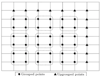
Figure 3. Types of points in non-polynomial spline group explicit for Nx= Ny= 8.

ordered and has property-A() _{[24]. Thus, the theory}

of block SOR is also applicable to the non-polynomial spline group explicit iterative method and, therefore, is convergent.

Here, the computational complexity of the non-polynomial spline iterative method is examined to show the eciency of the proposed method. We assume that the solution domain is discretized into even intervals, Nxand Ny in x- and y-directions, respectively.

There-fore, we have (nx 1)(ny 1) Grouped Points (GP)

and (nx+ ny 1) ungrouped points (UGP), where

nx = Nx 1 and ny = Ny 1. This can be shown

as in Figure 3.

The estimation of this computational complexity is based on the arithmetic operations performed at each iteration for the Additions/Substractions (A/S) and Multiplications/Divisions (M/D) operations [6]. Therefore, the number of operations required per iteration for non-polynomial spline group explicit is given as in Table 1. The total number of arithmetic operations can be obtained by multiplying the number of arithmetic operations for each iteration with the number of iterations.

5. Numerical results

In this section, some benchmark test problems with the known exact solution are solved by the proposed combination of Non-polynomial Spline and Group Ex-plicit iterative method (NSGE), which is approximately

Table 1. The number of arithmetic operations per iteration for non-polynomial spline group explicit iterative method.

Internal points A/S M/D

GP (nx 1)(ny 1) 8(nx 1)(ny 1) 8(nx 1)(ny 1)

UGP (nx+ ny 1) 8(nx+ ny 1) 6(nx+ ny 1)

(8)

O(k2_+h4_{). To demonstrate the method is of the fourth}

order; so, we take k = h2_{. Relation (12) is suitable for}

solving Eq. (1), provided that it satises the consis-tency condition; that is, when + 2 + = 1, which is equivalent to equation tan(!=2) = !=2. This equation has innite numbers or roots, the smallest positive nonzero root being given by ! = 8:986818916 [25].

The results are then compared with those ob-tained by the:

Combination of non-polynomial spline with stan-dard point Gauss-Seidel iterative method (NSPT);

Combination of Central Dierence scheme with Group Explicit iterative method (CDGE).

where the CDGE scheme is of O(h2 _{+ k}2_{), which}

can be derived by substituting the partial derivative into Eq. (1) with the central dierence approximation, similar to the one adopted in [6]. In all cases, we assume that u(0) _{= 0 as the initial guess and the iterations are}

stopped when the estimated error is below tolerance, that is, when ju(s+1) _u(s)_{j 10} 12 _{is achieved.}

All the experiments are implemented on a PC with Intel(R) Core(TM)2 Quad CPU Q9400 @ 2.66 GHz, 3 GB of RAM running Windows 7 using Matlab 7.10.0 (R2010a).

Example 1. Consider the following two-dimensional Poisson's equation:

@2_u

@x2 +

@2_u

@y2 = (x2+ y2)exy; 0 < x; y < 1;

with Dirichlet boundary conditions satisfying exact solution u(x; y) = exy_{. The solutions can be obtained}

by substituting the above approximations (Eqs. (14a)-(14c)), ^ml;m = ^ml+1;m = ^ml 1;m = 0 and g(x; y) =

(x2_{+ y}2_)exy _{into the dierence scheme (Eq. (26)) and}

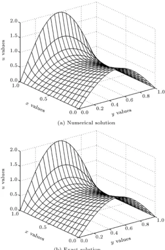
solved as in Section 4. The graphs of the numerical and exact solutions are plotted in Figure 4(a) and (b), respectively, for h = 1=16 and k = 1=20. The max-imum errors and execution timings of NSGE method compared with those of NSPT method are tabulated in Table 2, while the maximum errors and execution

Figure 4. Simple Poisson's equation for h = 1=16 and k = 1=20.

timings obtained by the proposed NSGE method and the existing central dierence group scheme CDGE are shown in Table 3. The total arithmetic operations needed for both NSGE and NSPT are displayed in Table 4.

Example 2. Consider the convection-diusion equa-tion:

@2_u

@x2 +

@2_u

@y2 =

@u

@x; 0 < x; y < 1;

where constant > 0 represents the ratio of convection

Table 2. Maximum absolute errors for Example 1 (k = h2_).

h k

O(k2_{+ h}4_{)-method, NSGE} _O(k2_{+ h}4_{)-method, NSPT}

Maximum absolute errors

Time (seconds)

1

4 161 0.66375E-05 0.01 0.66375E-05 0.01

1

8 641 0.41322E-06 0.12 0.41317E-06 0.22

1

16 2561 0.24756E-07 13.00 0.23968E-07 17.64 1

(9)

Table 3. Maximum absolute errors for Example 1 (k = h2_).

h k

O(k2_{+ h}4_{)-method, NSGE} _O(h2_{+ k}2_{)-method, CDGE}

Time (seconds)

1

4 161 0.66375E-05 0.01 0.10415E-03 0.05

1

8 641 0.41322E-06 0.12 0.27036E-04 0.12

1

16 2561 0.24756E-07 13.00 0.67558E-05 11.25 1

32 10241 0.23371E-07 1520.14 0.16749E-05 1425.48

Table 4. Total arithmetic operations needed to generate the above results.

h k O(k

2_{+ h}4_{)-method, NSGE} _O(k2_{+ h}4_{)-method, NSPT}

Number of iterations

Total arithmetic operations

1

4 161 224 153,664 311 167,940

1

8 641 2408 16,658,544 4124 21,824,208

1

16 2561 32362 1,963,143,644 56953 2,614,142,700 1

32 10241 445889 225,308,603,478 783787 298,274,845,572

to diusion and the exact solution is given by: u(x; y)=ex2 sin y

sinh h

2e 2 sinh x+sinh (1 x)

i ; where 2 ₌2 ₊ 2

4 . The boundary conditions can

be obtained from the exact solution. (4 4) matrix system can be obtained by substituting D00 = ,

D10 = D20 = 0 and Gl;m = Gl+1;m = Gl+1;m+1 =

Gl;m+1= 0 into Eq. (30). The graphs of the numerical

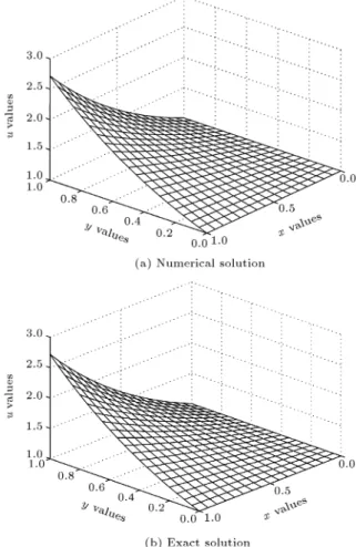
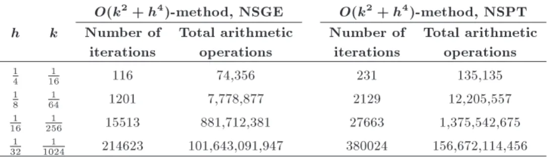
and exact solutions are plotted in Figure 5(a) and (b), respectively, for = 10, h = 1=16, and k = 1=20. Table 5 displays the comparison of maximum errors and execution timings of the NSGE method with those of the NSPT method. Meanwhile, Table 6 depicts the maximum errors and execution timings obtained by the proposed NSGE method compared with those of the existing central dierence group scheme CDGE [6]. Table 7 shows the total arithmetic operations needed for both NSGE and NSPT.

Example 3. Given the two-dimensional Poisson's equation in polar cylindrical coordinates in r z plane:

@2_u

@r2+

@2_u

@z2+

1 r

@u

@r=cosh z 5r cosh r+2(2+r2) sinh r

; where 0 < r; z < 1. The exact solution is u(r; z) = r2_{sinh r cosh z. The solutions can be approximated}

by replacing variables (x; y) by (r; z) and substituting g(r; z) = cosh z(5r cosh r +2(2+r2_{) sinh r) and D(r) =}

1

rinto the above scheme (Eq. (29)). The graphs of the

numerical and exact solutions are plotted in Figure 6(a) and (b), respectively, for h = 1=32, and k = 1=40. The maximum errors and execution timings of the proposed NSGE method compared with those of NSPT are displayed in Table 8, while the maximum errors

Figure 5. Convection-diusion equation for = 10 and h = 1=16.

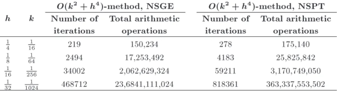
and execution timings of NSGE method compared with those of CDGE are tabulated in Table 9. The total arithmetic operations needed for both NSGE and NSPT are shown in Table 10.

(10)

Table 5. Maximum absolute errors for k = h2_{, and = 10.}

h k

Time (seconds)

1

4 161 0.35075E-00 0.01 0.35075E-00 0.03

1

8 641 0.21113E-01 0.07 0.21113E-01 0.09

1

16 2561 0.10942E-02 5.68 0.10942E-02 8.05

1

32 10241 0.68663E-04 657.93 0.68655E-04 889.61

Table 6. Maximum absolute errors for k = h2_{, and = 10.}

h k

Time (seconds)

1

4 161 0.35075E-00 0.01 0.24230E-00 0.04

1

8 641 0.21113E-01 0.07 0.78743E-01 0.06

1

16 2561 0.10942E-02 5.68 0.17155E-01 5.72

1

32 10241 0.68663E-04 657.93 0.43934E-02 544.28

h k

1

4 161 116 74,356 231 135,135

1

8 641 1201 7,778,877 2129 12,205,557

1

16 2561 15513 881,712,381 27663 1,375,542,675

1

32 10241 214623 101,643,091,947 380024 156,672,114,456

Table 8. Maximum absolute errors for k = h2_.

h k

Time (seconds)

1

4 161 0.18086E-01 0.04 0.18086E-01 0.04

1

8 641 0.60070E-03 0.21 0.60070E-03 0.23

1

16 2561 0.26865E-04 22.51 0.26866E-04 22.92 1

32 10241 0.77407E-05 2544.47 0.77324E-05 2694.46

Table 9. Maximum absolute errors for k = h2_.

h k

Time (seconds)

1

4 161 0.18086E-01 0.04 0.22704E-01 0.10

1

8 641 0.60070E-03 0.21 0.64553E-02 0.24

1

16 2561 0.26865E-04 22.51 0.17345E-02 20.40 1

(11)

h k

1

4 161 219 150,234 278 175,140

1

8 641 2494 17,253,492 4183 25,825,842

1

16 2561 34002 2,062,629,324 59211 3,170,749,050 1

32 10241 468712 23,6841,111,024 818361 363,337,553,502

Figure 6. Poisson's equation for h = 1=32 and k = 1=40.

6. Discussion

It can be observed that for all the model problems, the graph of the numerical solutions almost coincide with that of the exact solutions for dierent values of x and y, indicating that the computed solutions are in good agreement with the exact ones. As depicted in Tables 2, 5, and 8, the proposed NSGE converges faster than the existing NSPT, which is due to the lower computational complexity of the NSGE method. From Tables 3, 6, and 9, it can be seen that the proposed NSGE produces more accurate results than

CDGE which is of O(h2_+k2_{), while maintaining almost}

the same execution timings for all the examples. The total arithmetic operations needed for both NSGE and NSPT, for Examples 1, 2, and 3, are tabulated in Tables 4, 7, and 10. It is clear that the total number of arithmetic operations for NSGE is lower than that of NSPT in all cases due to the grouping strategies in the former method. The gains in the execution timings of NSGE over the NSPT are in the range of 26.3%-45.5% in Example 1, 22.2%-66.7% in Example 2, and 1.8-8.7% in Example 3.

7. Conclusions

In this paper, a new method, which incorporates a non-polynomial spline with the four-point group explicit iterative scheme, was formulated for solving the elliptic boundary value problems. The results show that the proposed method is capable of producing high-accuracy solutions with lesser computation timing compared to the non-polynomial spline standard point Gauss-Seidel method (NSPT) due to its lesser computational complexity. A more accurate result can be obtained by decreasing the step size. However, the computation time (computation cost) will be increased. In addition, the proposed method is superior to the original Central Dierence Group Explicit (CDGE) iterative method [6] in terms of accuracy, but with almost similar execution timings. In conclusion, the proposed method is a viable alternative approximation tool to solve the elliptic partial dierential equations.

Acknowledgment

The authors gratefully acknowledge the nancial sup-port from Universiti Sains Malaysia Research Univer-sity Grant (1001/JPEND/AUPE002) and FRGS Grant (203/PMATHS/6711321) and thank the reviewers for their valuable suggestions.

References

1. Aar~ao, J., Bradshaw-Hajek, B.H., Miklavcic, S.J. and Ward, D.A. \The extended-domain-eigenfunction method for solving elliptic boundary value problems

(12)

with annular domains", J. Phys. A: Math. Theor., 43, p. 185202 (2010).

2. He, W.-M. \High eective nite element algorithm for elliptic partial dierential equation", Appl. Math. Comput., 187(2), pp. 1567-1573 (2007).

3. Malavi-Arabshahi, S.M. and Dehghan, M. \Precon-ditioned techniques for solving large sparse linear systems arising from the discretization of the elliptic partial dierential equations", Appl. Math. Comput., 188(2), pp. 1371-1388 (2007).

4. Wang, Y.-M. and Guo, B.-Y. \Fourth-order compact nite dierence method for fourth-order nonlinear elliptic boundary value problems", J. Comput. Appl. Math., 221(1), pp. 76-97 (2008).

5. Xu, H., Zhang, C. and Barron, R. \A new numerical approach to solve an elliptic equation", Appl. Math. Comput., 171(1), pp. 1-24 (2005).

6. Yousif, W.S. and Evans, D.J. \Explicit group over-relaxation methods for solving elliptic partial dier-ential equations", Math. Comput. Simul., 28(6), pp. 453-466 (1986).

7. Abdullah, A.R. \The four point explicit decoupled group (EDG) method: A fast Poisson solver", Int. J. Comput. Math., 38, pp. 61-70 (1991).

8. Yousif, W.S. and Evans, D.J. \Explicit decoupled group iterative methods and their parallel implemen-tations", Parallel Alg. Appl., 7, pp. 53-73 (1995).

9. Abdullah, A.R. and Ali, N.H.M. \The comparative study of parallel strategies for the solution of elliptic PDE0s", Parallel Alg. Appl., 10, pp. 93-103 (1996).

10. Ali, N.H.M. and Lee, S.C. \Group accelerated over relaxation methods on rotated grid", Appl. Math. Comput., 191, pp. 533-542 (2007).

11. Ng, K.F. and Ali, N.H.M. \Performance analysis of explicit group parallel algorithms for distributed memory multicomputer", Parallel Comput., 34(6-8), pp. 427-440 (2008).

12. Saeed, A.M. and Ali, N.H.M. \On the convergence of the preconditioned group rotated iterative methods in the solution of elliptic PDEs", Appl. Math. Inf. Sci., 5(1), pp. 65-73 (2011).

13. Bickley, W.G. \Piecewise cubic interpolation and two-point boundary problems", Comput. J., 11(2), pp. 206-208 (1968).

14. Albasiny, E.L. and Hoskins, W.D. \Cubic spline solu-tions to two-point boundary value problems", Comput. J., 12(2), pp. 151-153 (1969).

15. Fyfe, D.J. \The use of cubic splines in the solution of two-point boundary value problems", Comput. J., 12(2), pp. 188-192 (1969).

16. Al-Said, E.A., Noor, M.A. and Rassias, T.M. \Cu-bic splines method for solving fourth-order obstacle problems", Appl. Math. Comput., 174(1), pp. 180-187 (2006).

17. Goh, J., Majid, A.A. and Ismail, A.I.M. \Numerical method using cubic B-spline for the heat and wave equation", Comput. Math. Appl., 62(12), pp. 4492-4498 (2011).

18. Goh, J., Majid, A.A. and Ismail, A.I.M. \A quartic B-spline for second-order singular boundary value problems", Comput. Math. Appl., 64(2), pp. 115-120 (2012).

19. Mohanty, R.K. and Gopal, V. \High accuracy cubic spline nite dierence approximation for the solution of one-space dimensional non-linear wave equations", Appl. Math. Comput., 218(8), pp. 4234-4244 (2011).

20. Ding, H.F., Zhang, Y.X., Cao, J.X. and Tian, J.H. \A class of dierence scheme for solving telegraph equation by new non-polynomial spline methods", Appl. Math. Comput., 218(9), pp. 4671-4683 (2012).

21. Gopal, V., Mohanty, R.K. and Jha, N. \New nonpoly-nomial spline in compression method of O(k2_{+ h}4_{) for} the solution of 1D wave equation in polar coordinates", Adv. Numer. Anal., 2013, 8 pages (2013).

22. Jha, N. and Mohanty, R.K. \Quintic hyperbolic non-polynomial spline and nite dierence method for nonlinear second order dierential equations and its application", J. Egyptian Math. Soc., 22(1), pp. 115-122 (2014).

23. Goh, J. and Ali, N.H.M. \High accuracy Spline Ex-plicit Group (SEG) approximation for two dimensional elliptic boundary value problems", Plos One, 10(7), pp. 1-13 (2015).

24. Young, D.M., Iterative Solution of Large Linear Sys-tems, pp. 140-171, Academic Press, New York (1971).

25. Jain, M.K. and Aziz, T. \Spline function approxima-tion for dierential equaapproxima-tions", Comput. Methods in Appl. Mech. Eng., 26(2), pp. 129-143 (1981).

Biographies

Joan Goh received her Bachelor of Science (Maths) with a minor in Management from Universiti Sains Malaysia in 2003. She received her MSc in Mathe-matics and completed her PhD in Numerical Analysis from Universiti Sains Malaysia, in 2007 and 2013, respectively. She continued her research at Universiti Sains Malaysia as a Postdoctoral Fellow in 2014. Norhashidah Hj Mohd Ali received her Bachelor of Science (Maths) with a minor in Information Sciences from Western Illinois University, USA. She received her MSc in Applied Mathematics from Virginia Tech, USA, and completed her PhD in Industrial Computing from Universiti Kebangsaan Malaysia in 1998. She has been with Universiti Sains Malaysia since 1990. Her research interests are mainly in the area of Numerical Partial Dierential Equations.