Classifying inputs and outputs in interval data envelopment analysis

(1)

134

Hossein Azizi1*, Alireza Amirteimoori2

1

Department of Applied Mathematics, Parsabad Moghan Branch, Islamic Azad University, Parsabad Moghan, Iran

2

Department of Applied Mathematics, Rasht Branch, Islamic Azad University, Rasht, Iran hazizi@iaupmogan.ac.ir; azizhossein@gmail.com

Abstract

Data envelopment analysis (DEA) is an approach to measure the relative efficiency of decision-making units with multiple inputs and multiple outputs using mathematical programming. In the traditional DEA, it is assumed that we know the input or output role of each performance measure. But in some situations, the type of performance measure is unknown. These performance measures are called flexible measures. In addition, the traditional DEA needs crisp input and output data which may not always be available in real world applications. This paper discusses the input or output role of flexible measures using the DEA in environments with interval inputs and outputs. The application of the proposed DEA models is shown with a real dataset.

Keywords: Data envelopment analysis; interval data; flexible measures

1- Introduction

Data envelopment analysis (DEA) was developed primarily for measuring the relative efficiency of peer decision-making units (DMUs) where multiple inputs and multiple outputs are available (Charnes et al., 1978, Banker et al., 1984). The DEA has been used in a variety of environments including the public sector, banking, insurance, agriculture, transport, power industry, and many other applications (Kao and Hwang, 2008, Jahanshahloo et al., 2004, Wang et al., 2009, Zhang et al., 2009, Du et al., 2010, Tavana et al., 2013, Kao et al., 2017, Eskelinen, 2017, Liu et al., 2017, Du et al., 2017, Fan et al., 2017, Wang et al., 2017, Amirteimoori et al., 2016). The conventional DEA analyses require a set of measures and it is assumed that the input or output role of measures is known. But in many situations, there are measures whose situation is flexible. For example, in the evaluation of research productivity in the university, like what has been discussed in Beasley (1990), Beasley (1995), there is always the question that whether the research income is an input or an output? In articles, many authors have suggested that it should be considered as an input because this is the money earned by the university and it is used for the same period. Others argue that this is an income obtained from the university, therefore it should be considered as an output. However, to obtain a higher efficiency score, some universities may consider the research income as an input and others see it as an output. The main question is how to decide about the role of research income for each university? Similarly, in a conventional study discussing the operational efficiency of bank branches for investment attraction, like what has been discussed inCook and Hababou (2001), Cook et al. (2000), a factor such as the number of high value customers can be considered either as input or output.

*Corresponding author.

Classifying inputs and outputs in interval data envelopment

analysis

Journal of Industrial and Systems Engineering Vol. 10, No. 2, pp 134-150

(2)

135

It can be said that in cases where there is ambiguity, the correct selection of the input or output role of a performance measure mainly depends on the fairest possible behavior with the DMU. Thus, the organization must adopt the fairest possible approach with the least opposition for efficiency evaluation. Bala and Cook (2003), and Cook and Zhu (2007) pointed to very similar questions in the context of the DEA. Bala and Cook (2003) studied the decision problem on the suitable situation of flexible measures when additional information is available. In particular, they studied a situation that consultants of bank branches present additional classification data and specify good or bad branches. The idea is that any flexible measure is given a situation so that obtained efficiency scores have the most consistency with expert opinion. A major problem in the method proposed by Bala and Cook (2003) is that additional information must be entered for making decisions on the situation of each variable. Cook and Zhu (2007) proposed a different approach for classification of flexible variables. They introduced a single model and a model that optimizes the cumulative efficiency of a set of DMUs. Toloo (2009) showed that the use of Cook and Zhu (2007) may lead to inaccurate efficiency scores in some cases due to a computational error by entering a large positive number to the model. He then proposed a revised model that did not need such a large positive number. Amirteimoori and Emrouznejad (2011) proposed a new model for working with flexible measures and demonstrated that the main disadvantage of the model proposed by Cook and Zhu (2007) is that it overestimates the efficiency. The proposed approach by Amirteimoori and Emrouznejad (2011) was extended to the slack-based model by Amirteimoori et al. (2013). Moreover, Amirteimoori and Emrouznejad (2012) showed that the modified model of Toloo (2009) is a special case of the model of Cook and Zhu (2007) and it is not applicable in many cases. For working with a flexible measure, Cook et al. (2006) developed a model that considers only a single factor and it ignores many flexible measures. This approach was extended to the mode of multiple flexible measures by Farzipoor Saen (2010).

The traditional DEA models assume that exact data are available for all inputs and outputs. In some applications, however, some of the factors may include imprecise data (Amirteimoori and Kordrostami, 2005, Kim et al., 1999, Smirlis et al., 2006, Khalili-Damghani et al., 2015, Jahed et al., 2015). The nature of these imprecise data depends on the characteristics of the particular problem (Kao and Liu, 2004, Kao and Liu, 2011, Liu, 2008). For example, they could be in the form of missing values, integer values, judgment data, fuzzy data, rank data, etc (Cooper et al., 2001, Kao and Liu, 2000a, Kao and Liu, 2000b, Amirteimoori and Kordrostami, 2014, Cook et al., 2012, Cook and Zhu, 2006). Various DEA models have been developed for dealing with imprecise data (Smirlis et al., 2006, Azizi, 2013b, Kao, 2006, Lozano and Villa, 2006, Liu, 2014). Farzipoor Saen (2011) extended the proposed model of Toloo (2009) for the media selection problem in the presence of both types of flexible factors and imprecise data. The proposed DEA models of Farzipoor Saen (2011) have some shortcomings: (1) They always overestimate or underestimate the efficiency; and (2) they are not applicable in many real cases. To overcome this problem, in this paper we extend the proposed approach of Amirteimoori and Emrouznejad (2011). We believe that this approach is an important contribution to the interval DEA discussion which has been less studied.

The paper is organized as follows. Section 2 presents the interval DEA models. Section 3 provides an interval DEA based approach for modeling production processes in the presence of flexible measures. In section 4, the DEA models of Farzipoor Saen (2011) are analyzed. Section 5 shows the applicability of the proposed DEA models for media selection in Iranian steel industry. Section 6 is the conclusion.

2- Background

2-1- Interval DEA models for measuring optimistic efficiency of DMUs

In DEA analysis, it is generally assumed that there are

n

production units, each using

m

inputs and producing

s

outputs. Specifically, the

j

th production unit consumes the values

0 ) , , ( ₁

r

≥ …

= j mj

j x x

X , 0

r

≠

j

X ( j =1,…,n), from the inputs, while it produces the values

0 )

,

(

₁

r

≥

…

=

j sj

j

y

Y

, 0

r

≠

j

Y ( j =1,…,n) from the outputs. In interval DEA, it is assumed that a few of the precise values of input

x

_ij and output

y

_rj are unknown. The only thing we know is that

(3)

136

they all fall in the upper and lower bounds of the range determined by intervals [ , Uij]

L ij x

x and ]

,

[y_rjL yU_rj ; where x_ijL >0 and y_rjL >0.

To deal with such an unreliable condition, the pair of linear programming models has been created as below, so as to produce the upper and lower bounds of optimistic efficiency for each DMU (Wang et al., 2005): . , , 1 ; , , 1 , 0 , , 1 , , , 1 , 0 s.t. max 1 1 1 1 m i s r v u x v n j x v y u y u i r m i L io i m i L ij i s r U rj r s r U ro r U o … = … = ≥ = … = ≤ − =

∑

= = = =

φ

(1) . , , 1 ; , , 1 , 0 , , 1 , , , 1 , 0 s.t. max 1 1 1 1 m i s r v u x v n j x v y u y u i r m i U io i m i L ij i s r U rj r s r L ro r L o … = … = ≥ = … = ≤ − =

∑

= = = =

φ

(2)

where

DMU

_o indicates the DMU under evaluation, v_i (i=1,…,m) and u_r (r=1,…,s) as the decision-making variables.

φ

_oU and

φ

_oL are optimistic efficiencies under the most favorable and the most unfavorable conditions for

DMU

_o, respectively. They form the optimistic efficiency interval

] , [ oU

L

o

φ

. If there is a set of weights that makes

φ

oU* =1, then

DMU

o is said to be DEA efficient or

optimistic efficient; otherwise it is called DEA non-efficient or optimistic non-efficient. The dual program of models (1) and (2) is as follow:

free. ; , , 1 , 0 , , , 1 , , , , 1 , s.t. min 1 1 U o j U ro n j U rj j L io U o n j L ij j U o n j s r y y m i x x

φ

λ

φ

λ

φ

… = ≥ … = ≥ … = ≤

∑

= = (3) free. ; , , 1 , 0 , , , 1 , , , , 1 , s.t. min 1 1 L o j L ro n j U rj j U io L o n j L ij j L o n j s r y y m i x x

φ

λ

φ

λ

φ

… = ≥ … = ≥ … = ≤

∑

= = (4)

If the classic technology with constant return to scale is used, then the Production Possibility Set (PPS) is defined as below:

(

)

        … = ≥ ≥ ≤ =

∑

= = n j Y Y X X Y X T _j n j U j j n j L j

j , , 0, 1, ,

,

1 1

λ

(5)

T

is a closed and convex set and the frontier points

T

are defined as efficient production frontier.

(4)

137

3- Flexible measures in production process

3-1- An axiomatic foundation

Assume that

n

DMUs are to be assessed in terms of

m

inputs and

s

outputs. Assume that

ij

x (i=1,…,m) and yrj (r=1,…,s) are the input and outputs values for DMUj ( j=1,…,n),

respectively. Furthermore, assume that

t

is the flexible measure

z

_kj (k =1,…,t), the input/output condition of which is undetermined; these measures might be taken into account as input in some DMUs and as output in some others.

With regard to generality of the subject now, assume that there are only three performance measures

X

,

Y

, and

Z

for each DMU in the assessment model. Assume that Tˆ is the PPS of technology under study. Several facts are assumed as below:

A1- Feasibility of observed data: (X_j,Y_j,Z_j)∈Tˆ for each j=1,…,n

A2- Unbounded ray: (X,Y,Z)∈Tˆ implicitly means that we have

β

(X,Y,Z)∈Tˆ for each

β

≥0. A3- Convexity: Assume (X′,Y′,Z′)∈Tˆ and (X′′,Y′′,Z′′)∈Tˆ, then for each

λ

∈[0,1] we have

T Z Y X Z

Y

X , , ) (1 )( , , ) ˆ ( ′ ′ ′ + −

λ

′′ ′′ ′′ ∈

λ

.

A4- Free disposability:(X,Y,Z)∈Tˆ,

X

′

≥

X

, Y′≤Y, (either Z′≥Z or Z′≤Z) imply that T

Z Y

X , , ) ˆ ( ′ ′ ′ ∈ .

A5- Minimal extrapolation: Tˆ is the intersection set of all T′s satisfying the postulates 1, 2, 3, and 4, and subject to the condition that each of the observed vectors(X_j,Y_j,Z_j)∈T′, j =1,…,n.

Now an algebraic representation is given for PPS of technology Tˆ in order to support axioms A1 to A5.

Theorem 1: The PPS Tˆ, true in axioms A1 to A5, is defined as follow:

(

)

      

      

… = ≥ ≥

≤ ≥

≤ =

∑

=

= =

=

n j

Z Z

Z Z Y

Y X

X Z

Y X T

j n

j

U j j

n

j L j j n

j U j j n

j

L j j

, , 1 , 0 ), or

either ( , ,

, , ˆ

1

1 1

1

λ

(6)

Proof: It is clear that Tˆ set is true in axioms A1 to A5. In order to see Tˆ is a minimal set; assume that T′ as well supports A1 to A5. We should show that (X,Y,Z)∈Tˆ implies that(X,Y,Z)∈T′. Consider the below representation for unit(X,Y,Z).

Y

X

n

j U j j n

j

L j j

≥

≤

∑

= =

1 1

λ

either

Z

n

j L j

j

≤

∑

=1

λ

or

Z

n

j

U j

j

≥

∑

=1

λ

For vector

λ

=(

λ

₁,

λ

₂,…,

λ

_n) of this representation, we define:

)

,

(

)

,

(

1 1

1

∑

₌ ₌ ₌

=

n

j j j

n

j j j

n

j j

X

j

Y

Z

Y

X

_λ _λ _λ

λ

It is clear that(X_λ,Y_λ,Z_λ)∈T′; a unit dominating over (X,Y,Z) referring to Pareto principle. Hence, we conclude that (X,Y,Z)∈T′ completes the proof.

(5)

138 3-2- Interval DEA models with flexible measures

According to definition of PPS (6) and the result of Theorem 1, the following DEA models are proposed for assessing the efficiency interval ofDMU_o. In these models, each DMU determines the condition of performance measure Z in favor of its own efficiency level:

, , s.t. min 1 1 U o n j U j j L o U o n j L j j U o y y x x ≥ ≤

∑

= =

λ

θ

λ

θ

(7.1) , either 1 L o U o n j L j

jz

θ

z

λ

≤

∑

= (7.2) free. ; , , 1 , 0 , or 1 U o j U o n j U j j n j z z

θ

λ

… = ≥ ≥

∑

= (7.3)

, , s.t. min 1 1 L o n j U j j U o L o n j L j j L o y y x x ≥ ≤

∑

= =

λ

θ

λ

θ

(8.1) , either 1 U o L o n j L j

jx

θ

z

λ

≤

∑

= (8.2) free. ; , , 1 , 0 , or 1 L o j L o n j U j j n j z y

θ

λ

… = ≥ ≥

∑

= (8.3)

The above-mentioned models for solution are not easy linear programs. Therefore, the following method discusses transformation of the mentioned models into a mixed integer linear program. For instance, we take into account transformation of the DEA model in the upper-bound of the efficiency interval. Similarly, the DEA model in the lower-bound of the efficiency interval can be transformed through the same procedure.

It should be noted that one and only one of the constraints of either (7.2) or (7.3) should satisfy performance measureZ. Assume that M is a large positive number. Now consider the following constraints: , 1 1

δ

θ

λ

z _oUz_oL M

n

j L j

j ≤ +

∑

= (9.1) , 2 1

δ

λ

z zU M

o n

j U

j

j ≤− +

−

_∑

= (9.2)

,

1

2 1

+

δ

=

(6)

139

.

1 ,

0 ,

₂

1

δ

∈

{

}

δ

(9.4) Selecting

δ

₁

=

0

leads to

δ

₂

=

1

, thus the constraint (9.2) is redundant and (9.1) is satisfied. It implicitly means that

z

_oL is selected as an input measure for DMU_o. Moreover, if we allow

δ

1

=

1

, then

δ

₂

=

0

, thus the constraint (9.1) is redundant and (9.2) is satisfied. In this case,

z

_oU is selected as an output measure for DMU_o. The models (7.1)-(8.3) can now be presented again as mixed integer linear programs as below:

free. ; , , 1 , 0 , 1 , 0 , , 1 , , , , s.t. min 2 1 2 1 2 1 1 1 1 1 U o j U o n j U j j L o U o n j L j j U o n j U j j L o U o n j L j j U o n j M z z M z z y y x x

θ

λ

δ

λ

δ

θ

λ

θ

λ

θ

… = ≥ } { ∈ = + + − ≤ − + ≤ ≥ ≤

∑

= = = = (10) free. ; , , 1 , 0 , 1 , 0 , , 1 , , , , s.t. min 2 1 2 1 2 1 1 1 1 1 L o j L o n j U j j U o L o n j L j j L o n j U j j U o L o n j L j j L o n j M z z M z z y y x x

θ

λ

δ

λ

δ

θ

λ

θ

λ

θ

… = ≥ } { ∈ = + + − ≤ − + ≤ ≥ ≤

∑

= = = = (11)

3-3- Generalization of the proposed models

Assuming that there are three performance measures includingX, Y, and Z, the DEA models of (10) and (11) were constructed (where the condition Z should be determined in DEA models). Now assume that there are multiple inputs x_ij (i=1,…,m) and multiple outputs y_rj (r =1,…,s) and several flexible measures

z

_kj (k =1,…,t). For generalization of the proposed interval DEA models, we allow that each DMU determine every flexible measure, in a way that some flexible measures are considered as input and some other as output, so as to maintain its best efficiency score. In this case, the interval DEA models are proposed as below:

(7)

140 free. ; , , 1 , 0 , , , 1 , 1 , 0 , , , , 1 , 1 , , , 1 , , , , 1 , , , , 1 , , , , 1 , s.t. min 2 1 2 1 2 1 1 1 1 1 U o j k k k k k U ko n j U kj j k L ko U o n j L kj j U ro n j U rj j L io U o n j L ij j U o n j t k t k t k M z z t k M z z s r y y m i x x

θ

λ

δ

λ

δ

θ

λ

θ

λ

θ

… = ≥ … = } { ∈ … = = + … = + − ≤ − … = + ≤ … = ≥ … = ≤

∑

= = = = (12) free. ; , , 1 , 0 , , , 1 , 1 , 0 , , , , 1 , 1 , , , 1 , , , , 1 , , , , 1 , , , , 1 , s.t. min 2 1 2 1 2 1 1 1 1 1 L o j k k k k k L ko n j U kj j k U ko L o n j L kj j L ro n j U rj j U io L o n j L ij j L o n j t k t k t k M z z t k M z z s r y y m i x x

θ

λ

δ

λ

δ

θ

λ

θ

λ

θ

… = ≥ … = } { ∈ … = = + … = + − ≤ − … = + ≤ … = ≥ … = ≤

∑

= = = = (13)

4- Analysis of Farzipoor Saen’s (2011) DEA models

In this section, we analyze Farzipoor Saen’s (2011) DEA model which has been proposed as below:

.

,

1 ;

,

1 ,

0 ,

,

1 ,

0 },

1 ,

0 ,

,

1 ),

1 (

,

1 ,

0 ,

1 ,

,

1 ,

0

2 s.t.

2 max

1 1 1 1 1 1 1 1

m

i

s

r

v

t

k

d

t

k

d

t

k

d

z

x

v

n

j

z

x

v

z

y

z

y

i r k k k k k k k k k t k L ko k m i L io i t k L kj k m i L ij i t k U kj k s r U rj r t k U ko k s r U ro r U o

…

=

…

=

≤

…

=

≤

{

∈

…

=

−

+

≤

…

=

≤

=

+

…

=

≤

−

+

=

∑

= = = = = = = =

µ

γ

σ

γ

σ

γ

σ

µ

σ

µ

ϕ

(14)

(8)

141

.

,

1 ;

,

1 ,

0 ,

,

1 ,

0 },

1 ,

0 ,

,

1 ),

1 (

,

1 ,

0 ,

1 ,

,

1 ,

0

2 s.t.

2 max

1 1 1 1 1 1 1 1

m

i

s

r

v

t

k

d

t

k

d

t

k

d

z

x

v

n

j

z

x

v

z

y

z

y

i r k k k k k k k k k t k U ko k m i U io i t k L kj k m i L ij i t k U kj k s r U rj r t k L ko k s r L ro r L o

…

=

…

=

≤

…

=

≤

{

∈

…

=

−

+

≤

…

=

≤

=

+

…

=

≤

−

+

=

∑

= = = = = = = =

µ

γ

σ

γ

σ

γ

σ

µ

σ

µ

ϕ

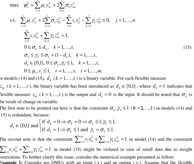
(15)

In models (14) and (15), d_k (k =1,…,t) is a binary variable. For each flexible measure

kj

z

(k=1,…,t), the binary variable has been introduced as d_k ∈{0,1}, where d_k =1 indicates that flexible measure

z

_kj (k=1,…,t) is the output and d_k =0 is the input. It should be noted that

σ

_k is the result of change in variable.

The first note to be pointed out here is that the constraint

σ

_k

,

γ

_k

≤

1

(k=1,…,t) in models (14) and (15) is redundant, because:







≤

=

≤

⇒

=

≤

⇒

=

⇒

=

{

∈

.

1 and

1

1 if

,

1 ,

1

0

0 if

and

}

1 ,

0

k k k k k k k k k

d

σ

γ

σ

γ

σ

The second note is that the constraint

1

+

∑

=

∑

₌ t₌

k L ko k m i L io

i

x

z

v

γ

in model (14) and the constraint

1

+

∑

=

∑

₌ t₌

k U ko k m i U io

i

x

z

v

γ

in model (15) might be violated in case of small data due to weight restrictions. To further clarify this issue, consider the numerical example presented as follow:

Example 1: Consider ten DMUs with an input (

x

) and an output (

y

). Assume that the flexible measure is (

z

), input and output of which should be known. The data have been shown in table 1.

Table 1. The data set for ten DMUs

DMU Input (

x

) Output (

y

) Flexible measure (

z

) 1 [0.031, 0.039] [0.0066, 0.00692] 0.00632

2 [0.0512, 0.0592] [0.00442, 0.004884] 0.00444 3 [0.0414, 0.0419] [0.00854, 0.009741] 0.00576 4 [0.0741, 0.0981] [0.00661, 0.007461] 0.00678 5 [0.0671, 0.0701] [0.00432, 0.006215] 0.00358 6 [0.0741, 0.0821] [0.00932, 0.00996] 0.00327 7 [0.0671, 0.0821] [0.00232, 0.006102] 0.00335 8 [0.0914, 0.0983] [0.00325, 0.005605] 0.00228 9 [0.0654, 0.0761] [0.0061, 0.006993] 0.0063 10 [0.048906, 0.06016] [0.00535, 0.007654] 0.00375

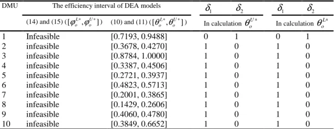
We first implement the DEA models proposed by Farzipoor Saen (2011) (DEA models (11) and (15)) for ten DMUs, so as to determine the condition of flexible measure. Regarding to table 2, it can be seen that DEA models proposed by Farzipoor Saen (2011) are infeasible for all the DMUs. We then implement the DEA models proposed in this paper, so as to determine the condition of flexible measure. Regarding to table 2, it is clear that the DEA models proposed in this paper have determined the condition of flexible measure quite manifestly. Furthermore, the efficiency interval obtained by DEA models (10) and (11) has been shown in table 2. For this numerical example, M =1 has been specified.

(9)

142 Table 2. Results

DMU The efficiency interval of DEA models

1

δ

2

δ

1

δ

2

(14) and (15) ([ ∗, oU∗] L

o ϕ

ϕ ) (10) and (11) ([ ∗, U∗]

o L

o θ

θ ) _{In calculation} U∗

o

θ

In calculation

θ

_oL∗

1 Infeasible [0.7193, 0.9488] 0 1 0 1 2 infeasible [0.3678, 0.4270] 1 0 1 0 3 infeasible [0.8784, 1.0000] 1 0 1 0 4 infeasible [0.3387, 0.4506] 1 0 1 0 5 infeasible [0.2721, 0.3937] 1 0 1 0 6 infeasible [0.4823, 0.5713] 1 0 1 0 7 infeasible [0.2001, 0.3865] 1 0 1 0 8 infeasible [0.1429, 0.2606] 1 0 1 0 9 infeasible [0.4060, 0.4780] 1 0 1 0 10 infeasible [0.3849, 0.6652] 1 0 1 0

Another major flaw in Farzipoor Saen’s (2011) DEA models is to always estimate efficiency either too higher or too lower. This issue will be illustrated through a numerical example in the next section.

5-An empirical example

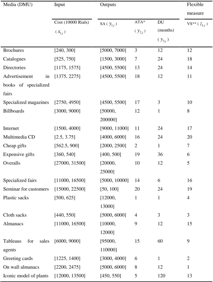
Selecting a medium in steel industry, Sepahan Industrial Group Co. (SIG) (Farzipoor Saen, 2011). A total of twenty media (DMUs) in SIG are evaluated in terms of one input and three outputs and a flexible measure mentioned in the following. The data set has been obtained from Farzipoor Saen’s (2011) paper shown in table 3. For this numerical example, M =106 has been specified.

Input 1

x

: Cost Outputs

1

y

: Size of Audiences (SA)

2

y

: Accuracy in Targeting of Audiences (ATA)

3

y : Durability of Media (DU) Flexible measure

1

(10)

143

Table 3. Relevant characteristics for 20 DMUs

Media (DMU) Input Outputs Flexible

measure

Cost (10000 Rials) (x₁_j)

SA (y₁_j) ATA* (y₂_j)

DU (months) (y₃_j)

VS** (z₁_j)

Brochures [240, 300] [5000, 7000] 3 12 12 Catalogues [525, 750] [1500, 3000] 7 24 18 Directories [1175, 1575] [4500, 5500] 13 24 14 Advertisement in

books of specialized fairs

[1375, 2275] [4500, 5500] 18 12 11

Specialized magazines [2750, 4950] [4500, 5500] 17 3 10 Billboards [3000, 9000] [50000,

200000]

12 1 8

Internet [1500, 4000] [9000, 11000] 11 24 17 Multimedia CD [2.5, 3.75] [4000, 6000] 16 24 20 Cheap gifts [562.5, 900] [2000, 2500] 2 1 7 Expensive gifts [360, 540] [400, 500] 19 36 6 Overalls [27000, 31500] [20000,

25000]

10 12 5

Specialized fairs [11000, 16500] [5000, 10000] 14 6 16 Seminar for customers [15000, 22500] [50, 100] 20 24 19 Plastic sacks [500, 625] [12000,

13000]

1 1 4

Cloth sacks [440, 550] [5000, 6000] 4 3 3 Almanacs [11000, 16500] [10000,

12000]

9 12 15

Tableaus for sales agents

[6000, 9000] [95000, 110000]

15 60 9

Greeting cards [1225, 1400] [3000, 4000] 6 1 2 On wall almanacs [2200, 2475] [5000, 6000] 8 12 1 Iconic model of plants [12000, 13500] [450, 550] 5 120 13

*Ranking such that 20 ≡ highest rank, … , 1 ≡ lowest rank (

14 , 2 10

, 2 13 ,

2 y y

y > >…> ).

**Ranking such that 20 ≡ highest rank, … , 1 ≡ lowest rank (

19 , 1 13 , 1 8 ,

1 z z

(11)

144

Media planning in SIG attempts to choose the best DMU. From the viewpoint of a media planner, VS might play the alternative role for great understanding of audiences. Hence, the study reasonably classifies it as output. However, it can be considered a flexible measure as well, since competitors acquire more information about SIG due to large amount of information presented to audiences. ATA and VS have been assessed at an ordinal scale, so that for instance, they rank the top in terms of ATA for

DMU

₁₃ (Seminar for customers) and for

DMU

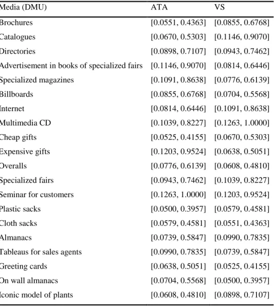
₁₄ (plastic bags) rank the lowest.

In order to convert strong ordinal preference information into interval data, assume that the preference intensity parameter and the ratio parameter have been estimated at

χ

=1.05 and

α

=0.05, respectively. By using a conversion technique described in Wang et al. (2005), interval estimation can be obtained for ATA and VS of each DMU, as shown in table 4. Farzipoor Saen (2011) has assumed, however, the preference intensity parameter about strong ordinal preference information has been given as

χ

=1.12. Obviously, the requirement

~

y

₂_j

≥

1 .

12 ~

y

₂_,_j₊₁ (or ~z₁j ≥1.12~z₁_,j₊₁) for

19 , , 13…

=

j is met. The requirement

~

y

₂_j

≥

1 .

12 y

~

₂_,_j₊₁ (or ~z₁j ≥1.12~z₁_,j₊₁) for j=1,…,12,

however, is not met. For instance, ~y2,18 =y21=3≥1.12×~y2,19 =1.12×2(y29)=2.24 is met, while 8

. 16 ) ( 15 12 . 1 ~ 12 . 1 16 ~

17 , 2 26

28

25 = y = ≥/ ×y = × y =

y is not met. Therefore, Should be selected

χ

quite carefully (Azizi, 2014, Azizi, 2013a).

Table 4. Interval estimation for 20 DMUs after conversion of ordinal preference information

Media (DMU) ATA VS

Brochures [0.0551, 0.4363] [0.0855, 0.6768] Catalogues [0.0670, 0.5303] [0.1146, 0.9070] Directories [0.0898, 0.7107] [0.0943, 0.7462] Advertisement in books of specialized fairs [0.1146, 0.9070] [0.0814, 0.6446] Specialized magazines [0.1091, 0.8638] [0.0776, 0.6139] Billboards [0.0855, 0.6768] [0.0704, 0.5568] Internet [0.0814, 0.6446] [0.1091, 0.8638] Multimedia CD [0.1039, 0.8227] [0.1263, 1.0000] Cheap gifts [0.0525, 0.4155] [0.0670, 0.5303] Expensive gifts [0.1203, 0.9524] [0.0638, 0.5051] Overalls [0.0776, 0.6139] [0.0608, 0.4810] Specialized fairs [0.0943, 0.7462] [0.1039, 0.8227] Seminar for customers [0.1263, 1.0000] [0.1203, 0.9524] Plastic sacks [0.0500, 0.3957] [0.0579, 0.4581] Cloth sacks [0.0579, 0.4581] [0.0551, 0.4363] Almanacs [0.0739, 0.5847] [0.0990, 0.7835] Tableaus for sales agents [0.0990, 0.7835] [0.0739, 0.5847] Greeting cards [0.0638, 0.5051] [0.0525, 0.4155] On wall almanacs [0.0704, 0.5568] [0.0500, 0.3957] Iconic model of plants [0.0608, 0.4810] [0.0898, 0.7107]

(12)

145

By applying interval DEA models (14) and (15), the optimistic efficiency score of DMUs are obtained, as shown in table 5. Regarding to table 5, it can be found out that two DMUs, i.e. DMUs number 6 and 8 based on DEA model (14) are optimistic efficient or DEA efficient. The remaining 18 DMUs are regarded as optimistic non-efficient with lower relative efficiency scores. The optimum level d can be seen in columns three and four of table 5. It is clear that except for

DMU

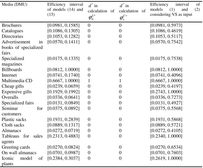
₈, all the DMUs take VS as input. In addition, we evaluated the efficiency interval of DMUs alongside interval DEA models (1) and (2) by considering the value of VS as input. The results have been reported in the fifth column of table 5. It is quite obvious that estimation of efficiency interval in Farzipoor Saen’s (2011) DEA models is not identical to estimation of efficiency interval in models (1) and (2) by considering VS as input. In fact, Farzipoor Saen’s (2011) DEA models are often inapplicable in real situations.

Table 5. The efficiency interval and the condition of flexible measure for 20 DMUs through Farzipoor Saen’s

(2011) models Media (DMU) Efficiency interval

of models (14) and (15)

*

d in

calculation of

∗

L o

ϕ

*

d in

calculation of

∗

U o

ϕ

Efficiency interval of models (1) and (2) considering VS as input

Brochures [0.0981, 0.1585] 0 0 [0.0981, 0.5973] Catalogues [0.1086, 0.1305] 0 0 [0.1086, 0.4619] Directories [0.1053, 0.1282] 0 0 [0.1053, 0.5117] Advertisement in

[0.0570, 0.1411] 0 0 [0.0570, 0.7542]

Specialized magazines

[0.0175, 0.1335] 0 0 [0.0175, 0.7538]

Billboards [0.0812, 1.0000] 0 0 [0.0812, 1.0000] Internet [0.0741, 0.1740] 0 0 [0.0741, 0.4096] Multimedia CD [0.6667, 1.0000] 1 1 [0.6667, 1.0000] Cheap gifts [0.0239, 0.0659] 0 0 [0.0239, 0.4197] Expensive gifts [0.1929, 0.1992] 0 0 [0.2743, 1.0000] Overalls [0.0336, 0.0641] 0 0 [0.0336, 0.7273] Specialized fairs [0.0131, 0.0849] 0 0 [0.0131, 0.4927] Seminar for

customers

[0.0375, 0.0892] 0 0 [0.0375, 0.5568]

Plastic sacks [0.1931, 0.2839] 0 0 [0.1931, 0.5868] Cloth sacks [0.0889, 0.1317] 0 0 [0.0889, 0.5721] Almanacs [0.0272, 0.0719] 0 0 [0.0272, 0.4105] Tableaus for sales

agents

[0.2313, 0.4883] 0 0 [0.2340, 1.0000]

Greeting cards [0.0270, 0.0824] 0 0 [0.0270, 0.6534] On wall almanacs [0.0701, 0.0987] 0 0 [0.0701, 0.7603] Iconic model of

plants

[0.2384, 0.3037] 0 0 [0.2619, 1.0000]

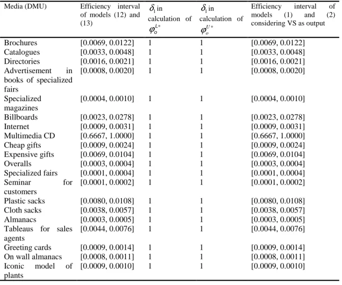
At this stage, we obtain the optimistic efficiency interval score of DMUs by applying interval DEA models (12) and (13), as shown in second column of table 6. From the perspective of optimistic efficiency, a DMU, i.e.

DMU

₈ based on DEA model (12) is optimistic efficient or DEA efficient. The remaining 19 DMUs are regarded as optimistic non-efficient with lower relative efficiency scores. In addition, the input/output behavior of VS level can be seen in table 6. It is quite obvious that our proposed interval DEA models define VS as output measure. Moreover, the efficiency interval of DMUs has been reported in the fifth column of table 6 by considering the VS level as

(13)

146

output using interval DEA models (1) and (2). The efficiency interval obtained from interval DEA models (1) and (2) is not completely identical to that obtained from interval DEA models (12) and (13). Hence, the media planner concludes that higher the VS the better.

Table 6. The efficiency interval and the condition of flexible measure for 20 DMUs through proposed DEA

models Media (DMU) Efficiency interval

of models (12) and (13)

1

δ

in

calculation of

∗

L o

ϕ

1

δ

in

calculation of

∗

U o

ϕ

Efficiency interval of models (1) and (2) considering VS as output

Brochures [0.0069, 0.0122] 1 1 [0.0069, 0.0122] Catalogues [0.0033, 0.0048] 1 1 [0.0033, 0.0048] Directories [0.0016, 0.0021] 1 1 [0.0016, 0.0021] Advertisement in

[0.0008, 0.0020] 1 1 [0.0008, 0.0020]

Specialized magazines

[0.0004, 0.0010] 1 1 [0.0004, 0.0010]

Billboards [0.0023, 0.0278] 1 1 [0.0023, 0.0278] Internet [0.0009, 0.0031] 1 1 [0.0009, 0.0031] Multimedia CD [0.6667, 1.0000] 1 1 [0.6667, 1.0000] Cheap gifts [0.0009, 0.0024] 1 1 [0.0009, 0.0024] Expensive gifts [0.0069, 0.0104] 1 1 [0.0069, 0.0104] Overalls [0.0003, 0.0004] 1 1 [0.0003, 0.0004] Specialized fairs [0.0001, 0.0004] 1 1 [0.0001, 0.0004] Seminar for

customers

[0.0001, 0.0002] 1 1 [0.0001, 0.0002]

Plastic sacks [0.0080, 0.0108] 1 1 [0.0080, 0.0108] Cloth sacks [0.0038, 0.0057] 1 1 [0.0038, 0.0057] Almanacs [0.0003, 0.0005] 1 1 [0.0003, 0.0005] Tableaus for sales

agents

[0.0044, 0.0076] 1 1 [0.0044, 0.0076]

Greeting cards [0.0009, 0.0014] 1 1 [0.0009, 0.0014] On wall almanacs [0.0008, 0.0011] 1 1 [0.0008, 0.0011] Iconic model of

plants

[0.0009, 0.0010] 1 1 [0.0009, 0.0010]

6- Conclusions

One assumption of traditional DEA models is that any performance measure is specified as an input or output. In the measurement of the real world performance, there are performance measures that are flexible. Moreover, the DEA is sometimes faced with the situation of imprecise data due to uncertainty. In this paper, we developed interval DEA models for calculating the efficiency interval of DMUs with flexible measures and interval data. The proposed interval DEA models were studied based on axioms. In these models, each DMU determines the flexible measure situation in favor of its efficiency level. The proposed DEA approach and the obtained interval DEA models were finally tested with two numerical examples including an example about media selection.

Compared with the DEA models of Farzipoor Saen (2011), the proposed interval DEA models are more easily solved and implemented for each scale of data. However, the DEA models of Farzipoor Saen (2011) are not feasible for small data and many other actual data. Moreover, the proposed interval DEA models give a correct efficiency interval for each DMU. Most importantly, the proposed interval DEA models correctly identify the situation of flexible measures. Therefore, the evaluation result is more comprehensive and suitable than the DEA models of Farzipoor Saen (2011). It is hoped that this study can add the richness of DEA theory and present alternative methods for performance measurement and input/output classification in the interval DEA.

(14)

147 Acknowledgement

Professor Alireza Amirteimoori would like to thank the financial support by Rasht branch, the Islamic Azad University, under grant number 4.5830. The authors are grateful for helpful suggestions and comments made by anonymous reviewer on an earlier version of the paper.

References

Amirteimoori, A. & Emrouznejad, A. 2011. Flexible measures in production process: A DEA-based approach. RAIRO - Operations Research, 45, 63-74.

Amirteimoori, A. & Emrouznejad, A. 2012. Notes on “Classifying inputs and outputs in data envelopment analysis”. Applied Mathematics Letters, 25, 1625-1628.

Amirteimoori, A. & Emrouznejad, A. & KHOSHANDAM, L. 2013. Classifying flexible measures in data envelopment analysis: A slack-based measure. Measurement, 46, 4100-4107.

Amirteimoori, A. & Kordrostami, S. 2005. Multi-component efficiency measurement with imprecise data. Applied Mathematics and Computation, 162, 1265-1277.

Amirteimoori, A. & Kordrostami, S. 2014. Data envelopment analysis with discrete-valued inputs and outputs. Expert Systems, 31, 335-342.

Amirteimoori, A., Kordrostami, S. & Azizi, H. 2016. Additive models for network data envelopment analysis in the presence of shared resources. Transportation Research Part D: Transport and

Environment, 48, 411-424.

Azizi, H. 2013a. A note on “A decision model for ranking suppliers in the presence of cardinal and ordinal data, weight restrictions, and nondiscriminatory factors”. Annals of Operations Research, 211, 49-54.

Azizi, H. 2013b. A note on data envelopment analysis with missing values: an interval DEA approach. The International Journal of Advanced Manufacturing Technology, 66, 1817-1823.

Azizi, H. 2014. A note on “Supplier selection by the new AR-IDEA model”. The International

Journal of Advanced Manufacturing Technology, 71, 711-716.

Bala, K. & Cook, W. D. 2003. Performance measurement with classification information: an enhanced additive DEA model. Omega, 31, 439-450.

Banker, R. D., Charnes, A. & Cooper, W. W. 1984. Some models for estimating technical and scale inefficiencies in data envelopment analysis. Management Science, 30, 1078-1092.

Beasley, J. E. 1990. Comparing university departments. Omega, 18, 171-183.

Beasley, J. E. 1995. Determining Teaching and Research Efficiencies. Journal of the Operational

Research Society, 46, 441-452.

Charnes, A., Cooper, W. W. & Rhodes, E. 1978. Measuring the efficiency of decision making units.

European Journal of Operational Research, 2, 429-444.

Cook, W. D., Green, R. & Zhu, J. 2006. Dual-role factors in data envelopment analysis. IIE

(15)

148

Cook, W. D. & Hababou, M. 2001. Sales performance measurement in bank branches. Omega, 29, 299-307.

Cook, W. D., Hababou, M. & Tuenter, H. H. 2000. Multicomponent Efficiency Measurement and Shared Inputs in Data Envelopment Analysis: An Application to Sales and Service Performance in Bank Branches. Journal of Productivity Analysis, 14, 209-224.

Cook, W. D., Harrison, J., Rouse, P. & Zhu, J. 2012. Relative efficiency measurement: The problem of a missing output in a subset of decision making units. European Journal of Operational Research, 220, 79-84.

Cook, W. D. & Zhu, J. 2006. Rank order data in DEA: A general framework. European Journal of

Operational Research, 174, 1021-1038.

Cook, W. D. & Zhu, J. 2007. Classifying inputs and outputs in data envelopment analysis. European

Journal of Operational Research, 180, 692-699.

Cooper, W. W., Park, K. S. & Yu, G. 2001. An Illustrative Application of Idea (Imprecise Data Envelopment Analysis) to a Korean Mobile Telecommunication Company. Operations Research, 49, 807-820.

Du, J., Liang, L., Chen, Y. & Bi, G.-B. 2010. DEA-based production planning. Omega, 38, 105-112.

Du, K., Xie, C. & Ouyang, X. 2017. A comparison of carbon dioxide (CO2) emission trends among provinces in China. Renewable and Sustainable Energy Reviews, 73, 19-25.

Eskelinen, J. 2017. Comparison of variable selection techniques for data envelopment analysis in a retail bank. European Journal of Operational Research, 259, 778-788.

Fan, Y., Bai, B., Qiao, Q., Kang, P., Zhang, Y. & Guo, J. 2017. Study on eco-efficiency of industrial parks in China based on data envelopment analysis. Journal of Environmental Management, 192, 107-115.

Farzipoor Saen, R. 2010. A new model for selecting third-party reverse logistics providers in the presence of multiple dual-role factors. The International Journal of Advanced Manufacturing

Technology, 46, 405-410.

Farzipoor Saen, R. 2011. Media selection in the presence of flexible factors and imprecise data.

Journal of the Operational Research Society, 62, 1695-1703.

Jahanshahloo, G. R., Amirteimoori, A. & Kordrostami, S. 2004. Multi-component performance, progress and regress measurement and shared inputs and outputs in DEA for panel data: an application in commercial bank branches. Applied Mathematics and Computation, 151, 1-16.

Jahed, R., Amirteimoori, A. & Azizi, H. 2015. Performance measurement of decision-making units under uncertainty conditions: An approach based on double frontier analysis. Measurement, 69, 264-279.

Kao, C. 2006. Interval efficiency measures in data envelopment analysis with imprecise data.

European Journal of Operational Research, 174, 1087-1099.

Kao, C. & HWANG, S.-N. 2008. Efficiency decomposition in two-stage data envelopment analysis: An application to non-life insurance companies in Taiwan. European Journal of Operational

(16)

149

Kao, C. & Liu, S.-T. 2000a. Data envelopment analysis with missing data: An application to University libraries in Taiwan. Journal of the Operational Research Society, 51, 897-905.

Kao, C. & Liu, S.-T. 2000b. Fuzzy efficiency measures in data envelopment analysis. Fuzzy Sets and

Systems, 113, 427-437.

Kao, C. & Liu, S.-T. 2004. Predicting bank performance with financial forecasts: A case of Taiwan commercial banks. Journal of Banking & Finance, 28, 2353-2368.

Kao, C. & Liu, S.-T. 2011. Efficiencies of two-stage systems with fuzzy data. Fuzzy Sets and Systems, 176, 20-35.

Kao T.-W., Simpson, N. C., Shao, B. B. M. & Lin, W. T. 2017. Relating supply network structure to productive efficiency: A multi-stage empirical investigation. European Journal of Operational

Research, 259, 469-485.

Khalili-Damghani, K., Tavana, M. & Haji-Saami, E. 2015. A data envelopment analysis model with interval data and undesirable output for combined cycle power plant performance assessment. Expert

Systems with Applications, 42, 760-773.

Kim, S.-H., Park, C.-G. & Park, K.-S. 1999. An application of data envelopment analysis in telephone officesevaluation with partial data. Computers & Operations Research, 26, 59-72.

Liu, D.-Y., Wu, Y.-C., Lu, W.-M. & Lin, C.-H. 2017. The Matthew effect in the casino industry: A dynamic performance perspective. Journal of Hospitality and Tourism Management, 31, 28-35.

Liu, S.-T. 2008. A fuzzy DEA/AR approach to the selection of flexible manufacturing systems.

Computers & Industrial Engineering, 54, 66-76.

Liu, S.-T. 2014. Restricting weight flexibility in fuzzy two-stage DEA. Computers & Industrial

Engineering, 74, 149-160.

Lozano, S. & Villa, G. 2006. Data envelopment analysis of integer-valued inputs and outputs.

Computers & Operations Research, 33, 3004-3014.

Smirlis, Y. G., Maragos, E. K. & Despotis, D. K. 2006. Data envelopment analysis with missing values: An interval DEA approach. Applied Mathematics and Computation, 177, 1-10.

Tavana, M., Khanjani Shiraz, R., Hatami-Marbini, A., Agrell, P. J. & Paryab, K. 2013. Chance-constrained DEA models with random fuzzy inputs and outputs. Knowledge-Based Systems, 52, 32-52.

Toloo, M. 2009. On classifying inputs and outputs in DEA: A revised model. European Journal of

Operational Research, 198, 358-360.

Wang, K., Zhang, J. & Wei, Y.-M. 2017. Operational and environmental performance in China's thermal power industry: Taking an effectiveness measure as complement to an efficiency measure.

Journal of Environmental Management, 192, 254-270.

Wang, Y.-M., Greatbanks, R. & Yang, J.-B. 2005. Interval efficiency assessment using data envelopment analysis. Fuzzy Sets and Systems, 153, 347-370.

(17)

150

arithmetic with an application to performance assessment of manufacturing enterprises. Expert

Systems with Applications, 36, 5205-5211.

Zhang, D., Li, X., Meng, W. & Liu, W. 2009. Measuring the performance of nations at the Olympic Games using DEA models with different preferences. Journal of the Operational Research Society, 60, 983-990.