Detection of Ground in Point-clouds Generated from Stereo-pair Images
Domen Mongus and Borut Žalik
University of Maribor, Faculty of Electrical Engineering and Computer Science E-mail: [email protected] and [email protected], http://gemma.uni-mb.si
Keywords:digital terrain model, mathematical morphology,Θ-mapping
Received:June 24, 2014
This paper proposes a new approach for constructing digital terrain models (DTM) from the point-clouds generated from airborne stereo-pair images. The method uses data decomposition based on the differential attribute profiles andΘ-mapping for the extraction of the most-contrasted connected-components. Their filtering is achieved based on multicriterion threshold function. The method is evaluated by comparing the output DTM with the reference Light Detection and Ranging data (LiDAR).
Povzetek: V ˇclanku predstavljamo novo metodo za konstrukcijo digitalnega modela reliefa iz oblaka toˇck, ki so generirani iz stereo-parov zraˇcnih fotografij. Metoda uporablja podatkovno dekompozicijo na osnovi diferencialnih atributnih profilov inΘ-mapiranja, s katerima doseže zaznavo najbolj kontrast-nih povezakontrast-nih komponent. Razpoznavo toˇck terena dosežemo z veˇckriterijskim pragovnim filtriranjem. Metode je evaluirana s primerjavo z digitalnim modelom reliefa, ustvarjenim iz podatkov LiDAR.
1
Introduction
Digital terrain models (DTMs) are essential part of various spatial analysis, geographic applications, and virtual reality systems [19, 6, 14]. In recent years, a considerable effort has been directed towards developing efficient approaches for accurate DTM generation.
When considering DTM generation from point-clouds, the most often used approaches can, according to the liter-ature, be classified as slope-based, linear prediction-based, and morphological methods [20, 9]. Slope-based methods [18, 21] achieve point-filtering by comparing the gradi-ents between neighbouring points. Consequentially, they have difficulties filtering points on step slopes and tend to smooth terrain undulations [20, 9]. Linear prediction-based methods, on the other hand, have difficulties filter-ing small and low objects as they rely on rough surface approximation to establish a liner prediction of the terrain [8, 2]. Actual filtering is usually achieved by observing the points’ residuals from the predicted surface. Preser-vation of sharp terrain details (e.g. ridges) can, therefore, be exposed as another weakness [20, 9]. By applying op-erations of mathematical morphology [5, 11, 4, 16], mor-phological filters proved to be fairly resistant to previously exposed drawbacks. However, they are severely depen-dent on the definition of the structuring element, as large objects (e.g. buildings) cannot be removed using a small structuring element, whilst large structuring element tends to flatten terrain details (e.g. mountain peaks) [20, 9, 5]. Several attempts have been proposed for optimal definition of a structuring element, the most efficient of which are based on a multi-scale filtering. A set of filters of differ-ent scales is used for this purpose and differdiffer-ent threshold values are usually defined for each of them. A progressive
filtering was proposed by Chen et al. [5], where threshold-ing is applied on height differences achieved by each filter. On the other hand, Mongus and Žalik [11] proposed data-filtering by iterating thin-plate splines towards the ground, where resolution is increased at each iteration by including points, filtered according to their residuals from the previ-ously estimated surface. This, so-called, hierarchical mul-tiresolution filtering has recently been improved by Chen et al. [4]. Pingel et al. [16] have, on the other hand, based their approach on the slope estimation achieved by linearly increasing filtering scale. Since all of these methods are adopted for processing high-resolution point-clouds con-taining vast amounts of points (e.g. LiDAR data), iterative approaches may not always be appropriate. Mongus and Žalik have [12] proposed an efficient multiscale approach that avoids iterations by using attribute filters based on the max-tree data structure. Although the method proves effi-cient when filtering LiDAR data, its accuracy is not guar-anteed when filtering low-resolution point-clouds (such as those generated from stereo-pair images) since it is based on the standard deviation of point heights.
2
Theoretical background
Letg:E→Rbe a regular grid, whereE⊂Z2andp
∈E is a grid point. Consider a level-setEl ⊂ Egiven by the
hight-levellasEl ={p|g[p] =l}. A connected
compo-nent fromEl is named a flat-zone ofg. A filter that acts
on flat-zones rather than individual grid-points is named a connected operator [17]. A connected operator can ei-der remove a zone (by merging it with some other flat-zones) or leave it perfectly preserved, but it cannot brake it. If the decision about which flat-zones to merge is based on some of their attributes, this type of operator is named an attribute filter [1]. Consider a set of all thresholded sets T ={Tl}ofg, each obtained by
Tl={p|g[p]≥l}. (1)
A peak connected componentCk
l ∈ Tl is defined by its
height levelland its component-at-level indexk. Let an at-tribute functionA(Ck
l)that estimates a particular attribute
ofCk
l, e.g. its area, diameter, or bounding-box. For
sim-plicity, letAbe increasing, thus, satisfying the condition Ck1
l1 ⊆C
k2
l2 →A(C
k2
l2 )≤A(C
k2
l2). An attribute filterγ
A a
acting ongis at a particular pointpdefined by
γAa(s)[p] =
_
{l|p∈Clk, A(C k
l)≥a}, (2)
where W
is supremum (i.e. the upper-bound). In other words, an attribute filterγA
a removes all the peak connected
components not satisfying an attribute threshold condi-tion a by assigning to each point p the maximal height-level at which it still belongs to a peak connected com-ponentCk
l withA(C k
l) ≥ a. Since ∀g, γ A
a(g) ≤ g, γaA
is an anti-extensive morphological filter named attribute opening. Its dual, an attribute closing φA
a, is defined as
γA
a(g) =−φAa(−g).
A decomposition named DAP or differential attribute profile∆has recently been proposed by Ouzounis et. al. [15]. ∆is based on progressive content reduction by fil-tering g at an increasing scale. Consider an ordered set of attribute thresholds a = {ai}, where i ∈ [0, I] and
ai−1< ai,∆is obtained by
∆A
a(g) ={γ
A
ai−1(g)−γ
A
ai(g)}, (3)
wherei∈[1, I]. Thus,∆A
a(g)is anI−long response
vec-tor registering the differences introduced by each particular γA
ai, whilstγ
A
aI(g)is a grid residual.
Recently, Mongus and Žalik [12] proposedΘ−mapping that registers the most-contrasted connected-components and estimates their arbitrary attributes by observing char-acteristic values contained in ∆A
a. Namely,Θ−mapping
estimates the most-contrasted connected-components from g by registering the maximal responses from ∆A
a(s)and
filtering scale at which they are obtained. Formally, Θ(g, A,a) :g→(g0, g◦), is atpgiven by
g0[p] =_∆A
a(g)[p], (4)
g◦[p] =^i|γaA
i−1(g)[p]−γ
A
ai(g)[p] =g
0[p], (5)
whereV
is infinum (i.e. the lower-bound). Consider a set of peak connected-componentsCp =
{Clp}containing a point p, i.e. Clp = Ck
l | p ∈ C k
l. The most-contrasted
connected-componentCp
maxwith the respect to the given
∆A
a(g)is identified by
max=_l|ag◦[p]−1≤A(Clp), (6)
wheremaxdefines the height-level of the most-contrasted connected-component. Note that possibly no response was obtained at a givenp, meaning that the corresponding peak connected-components are not in contrast against their sur-roundings and, therefore, belong to the grid residual, i.e. background. In any case, an arbitrary attribute ofCp
maxcan
then be measured and used as an attribute in multicriterion threshold definition.
3
Ground extraction from
point-clouds
The proposed method generates a digital terrain models from point-clouds obtained by stereo-pair images in the fol-lowing tree steps:
– Initializationis the first step of the method were input point-cloud is sampled into a grid,
– Point filtering is performed in the space of the most-contrasted connected-components obtained by Θ-mapping, and
– Construction of DTMis the final step of the method, where removed points are interpolated.
Each of these steps is discussed in continuation.
3.1
Initialization
In order to apply morphological operators on point-clouds, points are firstly sub-sampled into a regular grid g. The resolution of the grid Rg is defined by the point-density
DLasRg= 1.0/DL. When a particular grid-cell contains
more than one point, the hight level of the grid-point is de-fined by the lowest one since it has the highest probability of being a ground point. On the other hand, interpolation is used in order to estimate the hight levels of the undefined grid-points g[p∗] = U N DEF, obtained when there are
no points contained within the corresponding grid-cells. In our case, the height level at p∗ is estimated using inverse distance weighting (IDW) as [10]
g[p∗n] =
P
pn∈Wp
∗
ng[pn]d
−r pn
P
pn∈Wp
∗
nd
−r pn
, (7)
where pn is a grid-point from the neighbourhood Wp
∗
n of p∗n, anddpn is the Euclidean distance between p
∗
pn. Parameterrdefines the smoothness of the
tion. According to the evaluation of the spatial interpola-tion methods described in [3], accurate results are obtained whenWp∗ncontains at least three closest points andr= 2.
3.2
Ground filtering
In order to achieve extraction of the most-contrasted connected-components, the underlying definition of DAPs is given first. In compliance with demanded increasing property of the attribute used for grid decomposition, the proposed method constructs DAPs according to the area of the contained peak connected componentsA. An area threshold vectorais given as
a={20.0∗i}, (8)
wherei ∈ [0, I]. Note thata is given in square-metres, thus, its definition should be adjusted when the input point-cloud is not georeferenced. In any case, the following at-tributes of the most-contrasted connected-components are estimated byΘ-mapping:
– g0 describes the height difference or residual of the most-contrasted connected-component from its back-ground and is estimated by eq. 4,
– g◦ describes the area of the most-contrasted connected-components according to eq. 5,
– gc is a function describing shape-compactness of the most-contrasted connected-components and is esti-mated based on a well-known distance transformation as [13]
gc[p] = A(C
p max)
9π∗DT(Cmaxp )
, (9)
whereDT(Cp
max)is a function that estimates the
av-erage distance of a grid-point contained withinCp max
to the closest background point.
Afterg0,g◦, andgcare estimated, a set of ground
grid-pointsGis recognized with a multicriterion threshold func-tion given by
G={p|g0[p]≤tR, g◦[p]≤tS, gc[p]≤tC}, (10)
wheretR,tS, andtC are residual, size, and compactness
thresholds, respectively.
3.3
DTM construction
In the final step of the method, DTM is contracted by inter-polating the heights of the non-ground pointsN G=E/G using IDW, as given by eq. 7. However, usingr= 2may not always be appropriate as it may produce some sharp un-natural terrain features. Additional smoothing is, therefore, performed based on morphological openingγw, wherewis
a structuring element. In our case, final DTM is obtained by
DT M[p] =
g[p] ; g[p]−γw(g)≤Rg/2.0
γw(g)[p] ; otherwise
(11) wherewis box-shaped structuring element of size5×5.
4
Results
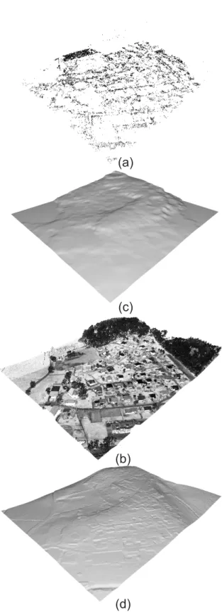
In order to evaluate the method, a point-cloud has been gen-erated from georeferenced stereo-pair image as proposed in [7] with approximately17.000points. Average point spac-ing was below3.1mand average absolute height error was 5.3min comparison to the reference data (see Fig. 1a). The reference data was acquired with LiDAR technology. The referenced point-cloud contained more than 1.6 millions of points with average point-spacing below than0.25m and average absolute height error below0.1m(see Fig. 1c).
The reference DTM was obtained with [12] and was used for the evaluation of the proposed method (see Figs. 1b and d). The results show that the proposed method is capable of removing important portion of noise as the average ab-solute difference of DTMs was lower than the average error of the point-clouds. Namely, the error is reduced to4.8m. However, significant portion of DTM’s details is missing due to the lower point-cloud resolution.
5
Conclusion
The paper proposes a new method for estimation of DTMs from point-clouds, generated by stereo-pair areal images. The method determines non-ground regions by estimating their geometrical characteristics, namely their sizes, shape compactness, and height differences from the background. As confirmed by the results,Θ-mapping provides sufficient solution for this purpose as great majority of errors were in-troduced by interpolation and lower data accuracy in com-parison to LiDAR data.
6
Acknowledgments
(a)
(b)
(c)
(d)
Figure 1:Estimation of DTM from (a and b) stereo-pair images and (c and d) the reference LiDAR data.
Acknowledgement
Acknowledgement text.
References
[1] E. Breen and R. Jones. Attribute openings, thinnings and granulometries.Computer Vision and Image Un-derstanding, 64(3):377–389, 1996.
[2] M. A. Brovelli, M. Cannata, and U. M. Longoni. LiDAR data filtering and DTM interpolation within GRASS.Transactions in GIS, 8(2):155–174, 2004.
[3] V. Chaplot, F. Darboux, H. Bourennane, S. Legué-dois, N. Silvera, and K. Phachomphon. Accuracy of interpolation techniques for the derivation of dig-ital elevation models in relation to landform types and data density.Geomorphology, 77 (1-2):126–141, 2006.
[4] C. Chen, Y. Li, W. Li, and H. Dai. A multiresolu-tion hierarchical classificamultiresolu-tion algorithm for filtering airborne LiDAR data. ISPRS Journal of Photogram-metry and Remote Sensing, 82:1–9, 2013.
[5] Q. Chen, P. Gong, D. Baldocchi, and G. Xie. Filter-ing airborne laser scannFilter-ing data with morphological methods. Photogrammetric Engineering & Remote Sensing, 73(2):175–185, 2007.
[6] R. Dinuls, G. Erins, A. Lorencs, I. Mednieks, and J. Sinica-Sinavskis. Tree species identification in mixed baltic forest using LiDAR and multispectral data. IEEE Journal of Selected Topics in Applied Earth Observations and Remote Sensing, 5(2):594– 603, 2012.
[7] M. Eineder, N. Adam, R. Bamler, N. Yague-Martinez, and H. Breit. Spaceborne spotlight SAR interfer-ometry with TerraSAR-X. IEEE Transactions on Geoscience and Remote Sensing, 47 (5):1524–1535, 2009.
[8] H. S. Lee and N. Younan. DTM extraction of LiDAR returns via adaptive processing. IEEE Transactions on Geoscience and Remote Sensing, 41(9):2063– 2069, 2003.
[9] X. Liu. Airborne LiDAR for DEM generation: some critical issues. Progress in Physical Geography, 32(1):31–49, 2008.
[10] C. D. Lloyd. Local Models for Spatial Analysis ( 2nd ed.). CRC Press, 2010.
[12] D. Mongus and B. Žalik. Computationally efficient method for the generation of a digital terrain model from airborne LiDAR data using connected operators. IEEE Journal of Selected Topics in Applied Earth Ob-servations and Remote Sensing, In press:1–12, 2013.
[13] R. S. Montero and E. Bribiesca. State of the art of compactness and circularity measures. International Mathematical Forum, 4 (25-28):1305–1335, 2009.
[14] A. O. Onojeghuo and G. A. Blackburn. Characteris-ing reedbeds usCharacteris-ing LiDAR data: Potential and lim-itations. IEEE Journal of Selected Topics in Ap-plied Earth Observations and Remote Sensing, (In press):1–7, 2012.
[15] G. K. Ouzounis, M. Pesaresi, and P. Soille. Differ-ential area profiles: Decomposition properties and ef-ficient computation. IEEE Transactions on Pattern Analysis and Machine Intelligence, 32(8):1533–1548, 2012.
[16] T. J. Pingel, K. C. Clarke, and W. A. McBride. An improved simple morphological filter for the terrain classification of airborne LIDAR data.ISPRS Journal of Photogrammetry and Remote Sensing, 77:21–30, 2013.
[17] P. Salembier and M. H. Wilkinson. Connected opera-tors: A review of region-based morphological image processing techniques.IEEE Signal Processing Mag-azine, 136 (6):136–157, 2009.
[18] J. Shan and A. Sampath. Urban DEM generation from raw LiDAR data: A labeling algorithm and its per-formance. Photogrammetric Engineering & Remote Sensing, 71(2):217–222, 2005.
[19] B. Sirmacek, H. Taubenbock, P. Reinartz, and M. Ehlers. Performance evaluation for 3-D city model generation of six different DSMs from air- and spaceborne sensors.IEEE Journal of Selected Topics in Applied Earth Observations and Remote Sensing, 5(1):59–70, 2012.
[20] G. Sithole and G. Vosselman. Experimental compari-son of filter algorithms for bare earth extraction from airborne laser scanning point clouds. ISPRS Journal of Photogrammetry and Remote Sensing, 59(1-2):85– 101, 2004.