ABSTRACT
The problem of slow drilling in deep shale formations occurs worldwide causing significant expenses to the oil industry. Bit balling which is widely considered as the main cause of poor bit performance in shales, especially deep shales, is being drilled with water-based mud. Therefore, efforts have been made to develop a model to diagnose drilling effectivity. Hence, we arrived at graphical correlations which utilized the rate of penetration, depth of cut, specific energy, and cation exchange capacity in order to provide a tool for the prediction of drilling classes.
This paper describes a robust support vector regression (SVR) methodology that offers superior performance for important drilling engineering problems. Using the amount of cation exchange capacity of the shaly formations and correlating them to drilling parameters such as the normalized rate of penetration, depth of cut, and specific energy, the model was developed. The method incorporates hybrid least square support vector regression into the coupled simulated annealing (CSA) optimization technique (LSSVM-CSA) for the efficient tuning of SVR hyper parameters. Also, we performed receiver operating characteristic as a performance indicator used for the evaluation of classifiers. The performance analysis shows that LSSVM classifier noticeably performs with high accuracy, and adapting such intelligence system will help petroleum industries deal with the well drilling consciously.
Keywords: Support Vector Regression, Shaly Formations, Coupled Simulated Annealing, Drilling Region Abdolhamid Sameni1* and Ali Chamkalani2
1 Chemical Engineering Faculty, Tarbiat Modares University, Tehran, Iran 2 Petroleum University of Technology, Ahwaz, Iran
Application of Least Square Support Vector Machine as a Mathematical
Algorithm for Diagnosing Drilling Effectivity in Shaly Formations
*Corresponding author
Abdolhamid Sameni
Email: [email protected] Tel: +98 92 0318 9417
Fax: +98 92 0318 9417
Article history
Received: May 03, 2016
Received in revised form: May 27, 2017 Accepted: July 19, 2017
Available online: January 07, 2018
INTRODUCTION
The remarkable portion of footage drilled occurs in shales; moreover, the drilling operation is performed at high ROP because shales are not rigid and stiff [10]. Due to chemical and mechanical factors, the cuttings stick together or to the bit. Therefore, the bit performance decreased which subsequently caused the drilling rate to decline
penetration (ROP) is global balling. Therefore, whatever prevents or minimizes the global balling can improve and optimize the drilling performance.
Bit Balling Investigations Review
Numerous research studies have considered the framework and the effect of bit balling, and drilling ineffectivity has subsequently been taken into account when drilling a shale formation. The bit balling study has been divided into mechanical and chemical approaches [5,7,8,10,14,31,34,46, 47]; the mechanical explanations ascribe balling to two problems [3]: (I) the difficulty in preserving fluid between the cutter and the cuttings lead to differential sticking of the cuttings to the bit (cutter), and (II) the dilatancy in the shear zone of the cuttings causes a drop in pore pressure within the cuttings, which leads to differential sticking. In addition, the chemical approach can be explained via two strategies [3]: (I) the tendency of drilling fluid to wet the surface of the bit, and (II) sticking of the cuttings by virtue of swelling, because hydrophilic cuttings try to imbibe water. This water imbibition is due to [3]: (1) cohesion among cuttings, and (2) adhesion to bit surfaces. Furthermore, the effect of other possible parameters on bit balling was also surveyed by exploring shale properties (such as cation exchange capacity (CEC)) [12,14,31], mud properties [5,7,8, 10,12,15,34,44,46,47,56], down-hole pressure [5, 7, 10, 12, 34, 46], and bit and cutter design [51, 56]. Other studies [1,3,6,8,17,21,22,26,27,29, 35,39,40,43,50,51,56] have been developed and proposed several normalized, dimensionless, and bit operating parameters for characterizing and diagnosing bit performance.
In this paper, in addition to the normalized rate
of penetration (ROPn), other parameters such as specific energy (Es) and depth of cut (Dcut) are also used to represent drilling performance. The field data used in the correlation are obtained from the southern Iranian oil field drilling wells at the time of drilling.
EXPERIMENTAL PROCEDURES
The Normalized Rate of Penetration
For making a comparison among the combined data from various drilled intervals, normalizing the ROP has been suggested [25]. The normalization is implemented by the following model[15]:
actual 2
60
n
b ROP ROP
WOB rpm
d
=
(1)
where, ROPactual , ROPn , WOB, db , and rpm are the actual rate of penetration, normalized rate of penetration, weight on bit, bit diameter, and rotary speed respectively.
Specific Energy
Pessier and Fear (1992) defined specific energy as the work done per unit volume of rock drilled. In the clean drilling, the specific energy decreases gradually, whereas in the balling region, the specific energy increases gradually. In general, a relatively low value implies efficient drilling and/ or weak rock, and a high value denotes ineffective drilling and/or strong rock [25]. The equation used by Pessier and Fear (992) to express specific energy is defined by:
120
( ) ( )
s WOB rpm Torque
E
Borehole Area Borehole Area ROP
π× ×
= +
× (2)
penetration.
A balled or worn bit requires higher specific energy than a new and/or clean bit for drilling the same rock under identical conditions. The difference between total torque and torque off-bottom is used to estimate bottom hole torque and to subsequently calculate the specific energy for all bit runs[25].
Depth of Cut
Smith (1998) defined the depth of cut as a supplementary parameter for surveying drilling performance:
5
cut ROP
D
rpm =
× (3) where Dcut, ROP, and rpm represent the depth of cut, rate of penetration, and rotary speed respectively.
Cation Exchange Capacity
The cation exchange capacity (CEC) is a tool to describe the electrolytic cation absorbability of a clay-rich rock onto pore surfaces. CEC measurement in oil and gas studies is usually used for shaliness evaluation of sedimentary formations [52]. However, the CEC of rocks in bore hole cannot directly and continuously be measured. The measurement of CEC is subject to laboratory or empirical correlations developed from logs. Typically, the oil and gas industries measure the CEC with an API-recommended methylene blue capacity test [33], but by taking the advantage of the logs derived, using correlations is a beneficial way. In the Appendix, the corresponding calculation and relationship for empirical correlations are described.
Support Vector Machines
Support vector machines (SVM) on the basis of statistical learning theory and structural risk minimization were introduced by Vapink in 1955 [48]. The SVM was constructed to maximize the minimum distance between the data which leads to an optimum hyper-plane. Assuming the objective is f (x) = ω.x + b, where the training set is given by {(xi,yi)}i=1,2,.,l, xi ∈ R is the input and yi∈{-1,1} is the output. For the linear separable case, SVM formulations appear to be:
1 1
1 1
+ ≥ + = +
+ ≥ + = +
T
i i
T
i i
w x b if y
w x b if y (4)
And for the non-separable case,
( )
( )
11 11∅ + ≥ + = +
∅ + ≥ + = +
T
i i
T
i i
w x b if y
w x b if y (5) where, ∅(x) maps the input data into a higher dimensional feature space. Support vector machines for multi-classification have been developed in different supervised classification applications for various issues [4,13,16,19,24,30,32,54,55,57]. A nonlinear kernel function computes the hyper-plane with a maximum margin of w2 between the classes. Standard SVM model utilizes the quadratic programming problem in the following equation:
( )
(
1)
1 2
1 0 1
=
+ ξ
∅ + = − ξ ξ ≥ = …
∑
lT
i i T
i i i i
min w w C
s.t y w x b , ,i , , l
(6)
where, C is the representative of the trade-off parameter.
By implementing Karush-Kuhn-Tucker (KKT) and using Lagrangian multipliers, αi, the quadratic programming problem can be solved. Consequently,
w can be obtained by using
( )
1
=
=
∑
s αt j t j∅ t jj
w y x
decision boundary.
Let donate tj (j=1, ..., s)j to the s support vectors. Then, one can rewrite:
( )
1
= α ∅
=
∑
t j t j t jS
w y x
j (7)
By taking the dual problem into account, the quadratic programming problem would be solved.
( )
(
)
1 1 1 2 0 0 = =α = − α α
≤ α ≤ ∀
α =
∑
∑
l
i i i j i j
j
i l
i i j
max Q y y K x , x
C , s.t . y
(8)
According to Mercer theorem, the kernel is similar to the following equation:
(
i j)
= ∅
( )
i T∅
( )
jK x ,x
x
x
(9)The general formulation for SVM is represented by:
( )
(
)
1
=
= α +
∑
l
i i i j j
y x sign y K x ,x b (10)
Least Square Support Vector Machines
Suykens and Vandewalle proposed a modified version of SVM called least square SVM (LS-SVM) [45]. Like SVM, LS-SVM has application in both regression and classification cases. LS-SVM has reduced the run time and shown more adaptivity. Moreover, LS-SVM draws attention because it employs an equality constraint-based formulation instead of using quadratic programming methods. In LS-SVMs, the regression appears as:
( )
(
)
2 1 1 21 0 1
= + ∅ + = − ≥ = …
∑
l T i i T i imin w w C e
s.t y w x b e , i ,i , , l
(11)
The Lagrangian equation is defined as follows:
(
)
2{
(
( )
)
}
1 1
1 1
2
, , ; T l l T
i i i i
i i
L w b eα W W C e α y w x b e
= =
= +
∑ ∑
− ∅ + − +(12) where, Lagrangian multipliers αi∈ R; if Lagrangian equation is differentiated with respect to w, b, αi,
and ei, and the conditions are applied, one may obtain:
( )
( )
(
)
1 1 0 0 0 0 10 1 1
, , ..
, , .. l
i i i i l i i i i i T
i i i
i
dL w y x
dw
dL y
db
dL Ce i l
de
dL y y w x b e i l
α α α α = = = → = ∅ = → = = → = = … = → = ∅ + − + = …
∑
∑
(13) Omitting e and w results in a KKT system:1 0 0 1 − =
Ω +
T
Y
Y C I (14)
where, C is a positive constant, and b is the bias.
(
)
(
)
(
)
( )
( )
(
)
1 11 1 1
1 1
= …
= … α = α … α
Ω = ∅ ∅ = ≤ ≤
v
T i
i T
ij i j i j i j i j
y y , , y , ,
, ,
y y x x y y K x ,x , i , j
(15) By applying the Mercer condition, the final result would be:
( )
(
)
1
=
= α +
∑
l
i i i j j
y x sign y K x , x b (16)
The most common kernel functions used in SVM are defined as follows [2,9]:
1. Linear kernel:
K x ,x
(
i j)
=
x x
i j (17)2. Polynomial kernel:
(
i j) (
= i j +)
d ∈Θ ≥0K x ,x x x C for d ,c (18)
3. Gaussian (RBF) kernel:
2
i j
i j 2
x x
K(x , x ) exp( )
2 − − = σ (19)
Coupled Simulated Annealing
Coupled simulated annealing (CSA) method was proposed by Xavier de Souza et al. in 2010 [53]. CSA features a new form of acceptance probability function that can be applied to an ensemble of optimizers. This approach considers several current states which are coupled together by their
energies in their acceptance probability function. Moreover, as it is distinct from classical simulated annealing (SA) techniques [1,29], parallelism is an inherent characteristic of this class of methods. The objective of creating coupled acceptance probability functions that comprise the energy of many current states, or solutions, is to generate more information when deciding to accept less favorable solutions.
The following equation describes the acceptance probability function A with coupling term ρ:
(
)
( )
( )
∞ θ ∞ − ρ → =
− + ρ i k i i i k E y exp T
A , x y
E y exp
T
(20)
where, Aθ(ρ, xi→yi) is the acceptance probability for every xi∈Θ, yi∈ ϒand ϒ ⊂ Θ. ϒ denotes the set of all possible states, and the set Θ ≡
{ }
xi iq=1 is presented as the set of current states of qminimizers; moreover, Tkac is the acceptance temperature parameter at time instant k. The variance σ2 of A
θ is equal to:
Θ ∀ ∈Θ
σ =
∑
A −q q
2 2
2 x
1 1 (21)
The coupling term ρ is given by:
( )
j i x k E y exp T ∞ ∈Θ − ρ =
∑
(22)Hence, CSA considers many current states in the set Θ, which is a subset of all possible solutions ϒ, and accepts a probing state yi based not only on the corresponding current state xi but by considering also the coupling term, which depends on the energy of all other elements of ϒ.
Performance Evaluation: Receiver
Operating Characteristic (ROC)
The ROC curve [18,21] shows the separation abilities of a binary classifier; by setting different
possible classifier thresholds, the data set is tested on misclassifications. If the plot has an area under the curve equal to 1 for the test data, a perfectly separating classifier is found (on that particular dataset); if the area is equal to 0.5, the classifier has no discriminative power at all.
The receiver operating characteristic (ROC) curve can be used to measure the performance of a classifier. ROC utilizes sensitivity and specificity analyses as given by:
TP
Sensitivity(%) 100
TP FN
= ×
+ (23)
TN
Specificity(%) 100
FP TN
= ×
+ (24)
where TP, TN, FP, and FN denote true positives, true negatives, false positives, and false negatives respectively.
True Positive (TP): An input is detected Effective as diagnosed by field observation, Effective.
True Negative (TN): An input is detected Ineffective as diagnosed by field observation, Ineffective. False Positive (FP): An input is detected Effective, but it is experimentally labeled Ineffective. False Negative (FN): An input is detected Ineffective, but it is experimentally labeled Effective.
blue halo surrounding the dyed solids, the end point is reached. Also, the CEC analyses can be performed at the well site with a minimum amount of equipment.
Results and Discussion
The data have been gathered from a shaly formation in one of the southern Iranian oilfields. The formations were drilled by a PDC bit using water-based mud. For evaluating and training the proposed model, the data set was divided into two categories. A randomly 12 data sets were selected for the testing stage, and the remaining data sets were used for training the diagnostic model. The method for measuring CEC is described in the preceding section. The input parameters to LS-SVM classifier include cation exchange capacity, normalized rate of penetration, depth of cut, and specific energy, whereas the output parameter represents the drilling effectivity/ ineffectivity. Furthermore, in the present study, it is tried to correlate CEC with the normalized rate of penetration, depth of cut, and specific energy in order to develop such classifications. It means that the effectivity/ineffectivity of drilling operations can be assessed by relating the aforementioned parameters.
In a separate study, the same dataset was exposed to the LS-SVR algorithm only (without the CSA algorithm), and the different parameters were optimized based on an exhaustive search. It was found out that it was not possible to reach the best solutions starting from arbitrary initial conditions. In particular, it is difficult to obtain the optimum choices of σ2and γ after starting with some discrete values. The solutions frequently become stuck in sub optimal local minima. These experiments
justified the use of a hybrid technique for LS-SVR parameter tuning. Then, these data were exposed to the hybrid CSA-LSSVM model. Figure 2 depicts the flowchart of the developed CSA-based hyper parameter determination approach for SVM. The k-fold method presented by Salzberg was applied to the experiments using a k value of 10 [38,20]. Thus, the dataset was split into 10 parts, with each part of the data sharing the same proportion of each class of data.
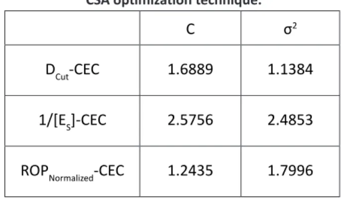
Due to fewer parameters to set and an excellent overall performance, the RBF is an effective option for kernel function [49,26]. Through an initial experiment without feature selection, the parameter values of the proposed CSA-LS-SVM approach were set as follows: T0 and Tkac were set to 1.0, and the range of the parameters of RBF kernel is selected arbitrary: σ2 = [0.001, 103] and C = [0.01, 104]. The optimal parameters for each
pair of the inputs are listed in Table 1.
Table 1: Optimal values of categories optimized by CSA optimization technique.
C σ2
DCut-CEC 1.6889 1.1384
1/[ES]-CEC 2.5756 2.4853
ROPNormalized-CEC 1.2435 1.7996
Figure 1: LSSVM model classify the drilling data into effective and ineffective for inputs of CEC-Dcut .
Figure 2: LS-SVM model classifies the drilling data into effective and ineffective for the inputs of CEC-1/Es.
As can be seen in Figure 3, the normalized rate of penetration was employed to distinguish effective bit cleaning from an ineffective drilling pattern.
Figure 3: LS-SVM model classifies the drilling data into effective and ineffective for the inputs of CEC-ROPn.
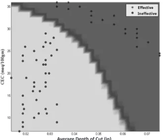
As Dcut and CEC increase simultaneously, effective drilling can be achieved. In other word, at low depth of cut, when the CEC is high, the drilling will be effective. Correlating CEC versus reciprocal of specific energy (Figure 2) shows a same trend as one described for Dcut vs. CEC. Since, specific energy is related to the strength of the rock being drilling and subsequently efficiency of the drilling operation, therefore a low value of specific energy implies an effective drilling operation, while high values shows an ineffective drilling process.
Figures 4 to 6 represent a general template detecting drilling ineffectivity. In addition, they can be used as a graphical correlation which utilizes ROPnormalized ,
Dcut , and the reciprocal of Es as tools for determining the functionality of drilling.
Figure 4: General template or graphical correlation for diagnosing drilling effectivity by inputs of CEC-Dcut .
Average Depth of Cut (in)
Table 2 performs a comparison between the observed and simulated drilling manner, where the inputs are Dcut- CEC. The predicted data show good agreement with the observed data with no false prognostication.
Table 2: Making a comparison between the observed and simulated drilling effectively for the inputs of DCUT-CEC.
NO. DCut CEC ObservedDrilling SimulatedDrilling 1 0.037535 36 Effective Effective
2 0.023459 11 Ineffective Ineffective
3 0.023459 8 Ineffective Ineffective
4 0.037535 35 Effective Effective
5 0.05161 30 Effective Effective
6 0.028151 10 Ineffective Ineffective
7 0.029324 22 Ineffective Ineffective
8 0.032843 35 Effective Effective
9 0.042226 33 Effective Effective
10 0.070377 25 Effective Effective
11 0.030028 26.8 Ineffective Ineffective
12 0.032843 9 Ineffective Ineffective
13 0.05161 30.5 Effective Effective
Also, Table 3 shows a comparison between the observed and simulated drilling effectively for the inputs of 1/[Es]-CEC.
Table 3: A comparison between the observed and simulated drilling effectively for the inputs of 1/[ES]-CEC.
NO. 1/[ES] CEC ObservedDrilling SimulatedDrilling 1 0.000277 28 Effective Effective 2 0.000238 33 Effective Effective 3 0.00012 27 Ineffective Ineffective 4 9.8E-05 16 Ineffective Ineffective 5 0.000159 36 Effective Effective 6 8.01E-05 24 Ineffective Ineffective 7 8.01E-05 9 Ineffective Ineffective 8 8.01E-05 9 Ineffective Ineffective 9 0.000238 30 Effective Effective 10 0.000218 32 Effective Effective 11 0.000218 30.5 Effective Effective 12 0.0001 25 Ineffective Ineffective
Figure 5: General template or graphical correlation for diagnosing drilling effectivity by inputs of CEC-1/Es.
Figure 8: Receiver Operating Characteristic curve for analysis of model performance for CEC-1/Es.
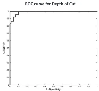
ROC curve for 1/[Average Specific Energy] Figure 7: Receiver Operating Characteristic curve for analysis of model performance for CEC-Dcut.
ROC curve for Depth of Cut
Moreover, Table 4 shows a comparison between the observed and simulated drilling effectively for the inputs of 1/[Es]-CEC.
Table 4: A comparison between the observed and simulated drilling effectively for the inputs of
ROPNormalized-CEC.
NO. ROPNormalized CEC ObservedDrilling- Simulated
Drilling-1 21.58898 26 Effective Effective
2 12.33656 35 Effective Effective
3 12.33656 36 Effective Effective
4 13.87863 35 Effective Effective
5 18.50484 33 Effective Effective
6 15.4207 34 Effective Effective
7 9.25242 17 Ineffective Ineffective
8 6.16828 15 Ineffective Ineffective
9 4.62621 19 Ineffective Ineffective
10 9.715041 20 Ineffective Ineffective
11 10.79449 9 Ineffective Ineffective
12 7.71035 11 Ineffective Ineffective
Furthermore, this comparison has been performed for 1/[Es]-CEC and ROPnormalized . For both, the results elucidate the high powerful ability of LS-SVM classifier.
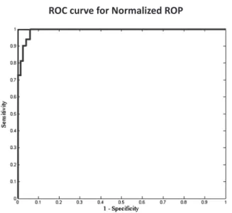
ROC curves are used to exhibit the performance and accuracy profile of classifications. The x-axis was set to (1-specificity), while y-axis was assigned to be sensitivity. As stated by Equations 19 and 20, one may obtain the following relations at the upper left-corner:
1 0
TP Then
Sensitivity FN
TP FN
= = → =
+ (26)
1-Specificity 1- TN 0 Then FP 0 FP TN
= = → =
+ (27)
CONCLUSIONS
This study presents a CSA-based approach capable of searching for the optimal parameters of SVM to diagnose drilling ineffectivity. Four parameters (in three pairs) were employed as tools to develop graphical correlations. The data were collected from Iranian oilfields drilled by PDC bit with water-based mud. For evaluating CSA-LS-SVM model, receiver operating characteristic (ROC) was adapted to monitor the model behavior. In addition, a comparison of the obtained results with the observed results demonstrates that the proposed CSA-LS-SVM works functionally and practically. Furthermore, CSA-LS-SVM is an intelligent system with a self-adapting attribute which helps drilling industry to upgrade drilling performance.
APPENDIX
To calculate CEC using log data, Rsh, ρma, φt, Fsh, and temperature (T) have to be estimated. First, one should calculate the counterion concentration, Qv
(meq/cc pore volume)as follows:
ROC curve for Normalized ROP
Figure 9: Receiver Operating Characteristic curve for analysis of model performance for CEC-ROPn.
max
sh v
sh
F Q
R B
= (1)
Bmax can be calculated using the following correlation derived from the experimental data collected by Waxman and Thomas (1975)[58].
2
max 0.0003 0.205 0.0929
B = − T + T− (2)
where, T(°C) is the temperature of the zone of interest , and Bmax (mho/m/(meq/cc)) is the maximum equivalent counterion conductance.
Qv is related to cation exchange capacity by:
(
1100)
tv
ma
CEC Q= φ ρφ
− (3)
where, φt (φt = φe + φB) is the total porosity, and φe is the effective porosity; φB is the fractional volume of water bound to shale, and ρma (gr./cc) is the density of rock matrix containing shale, and CEC (meq/100 gr.) is the cation exchange capacity. Using the approximation adapted in the dual water model, the total porosity is calculated as an average of density and neutron porosity, i.e.:
2
Neutron Density
t
φ
φ
φ
= + (4)The shale formation factor is then calculated by:
2
sh t
F =
φ
− (5)NOMENCLATURES
CEC : Cation Exchange Capacity
CSA : Coupled Simulated Annealing
db : Bit Diameter
Es : Specific Energy (kpsi)
FN : False Negative
FP : False Positive
KKT : Karush-Kuhn-Tucker
MBT : Methylene Blue Test
ROC : Receiver Operating Characteristic
ROP : Rate of Penetration [L/T]
ROPn : Normalized Rate of Penetration
rpm : Rotary Speed [L/T]
SVR : Support Vector Regression
TN : True Negative
TP : True Positive
WOB : Weight on Bit
REFERENCES
1. Aarts E. and Korst J., “Simulated Annealing and Boltzmann Machines,” New York: John Wiley and Sons, 1989, 415-417.
2. Abe S., “Support Vector Machines for Pattern Classification,” New York: Springer-Verlag
Springer, 2005, 1-467.
3. Aghassi A., “Investigation of Qualitative Methods for Diagnosis of Poor Bit Performance Using Surface Drilling Parameters,” MSc Dissertation,
Louisiana State University, 2003, 1-135. 4. Al-Anazi A. F. and Gates I. D., “Support
Vector Regression for Porosity Prediction in a Heterogeneous Reservoir: a Comparative Study,” Computations and Geosciences, 2010,
36, 1494–1503.
5. Allred R. B. and McCaleb S. B., “Rx for Gumbo Shale Drilling,” SPE 4233, The Sixth Conference
on Drilling and Rock Mechanics of Society of Petroleum Engineers of AIME, Dallas, TX, 1973.
6. Bible M., Lesage M., and Falconer I., “Method for Detecting Drilling Events from Measurement While Drilling Sensors,” USA Patent 4876886, Anadrill Inc., 1989.
7. Bland R., Haliday B., Illerhaus R., Isbell M., and et al., “Drilling Fluid and Bit Enhancement for Drilling Shales,” AADE Annual Technical Forum-Improvements in Drilling Fluids Technology, Houston, Texas, 1999.
8. Bourgoyne Jr., A. T., Chenevert M. E., Milheim K. K., and Young Jr. F.S., “Applied Drilling Engineering,” SPE Text Book Series, Richardson, TX, 1991.
9. Burges C. A. “Tutorial on Support Vector Machines for Pattern Recognition,” Data
Mining Knowledge Discovery 2, 1998, 121-167.
10. Chesser B. G. and Perricone A. C., “A Physicochemical Approach to the Prevention of Balling of Gumbo Shale,” SPE 4515, 48th Annual Fall Meeting of the Society of Petroleum
Engineers of AIME, Las Vegas, NV, 1973.
11. Cheatham C. A. and Nahm J. J., “Bit Balling in Water-Reactive Shale During Full-Scale Drilling Rate Test,” IADC/SPE 19926, IADC/SPE Conference, Houston, 1990.
12. Cheatham C. A., Nahm J. J., and Heikamp N. D. “Effect of Selected Mud Properties on Rate of Penetration – Full-Scale Shale Drilling Simulations,” SPE/IADC 13465, SPE/IADC Drilling Conference, New Orleans, LA. March, 1985.
14. Copper G. A. and Roy S., “Prevention of Bit Balling by Electro-Osmosis,” SPE 27882, SPE Western Regional Meeting, Long Beach, CA., 1994.
15. Demircan G., Smith J. R., and Bassiouni Z., “Estimation of Cation Exchange Using Log Data: Application to Drilling Optimization, Society of Petrophysicists and Well Log Analysts (SPWLA),” 41st Annual Logging Symposium, Dallas, Texas, June, 2000.
16. Du C. J. and Sun D. W., “Multi-Classification of Pizza using Computer Vision and Support Vector Machine,” Journal of Food Engineering, 2008, 86, 234-242.
17. Falconer I. G., Burgess T. M., and Sheppard M. C., “Separating Bit and Lithology Effects from Drilling Mechanics Data,” IADC/SPE 17191, Drilling Conference, Dallas, TX, 1988.
18. Fawcett T., “An Introduction to ROC Analysis,” Pattern Recognition Letters 27, 2006, 861-874. 19. Gao G. H., Zhang Y. Z., Zhu Y., and Duan G. H., “Hybrid Support Vector Machines-Based Multi-Fault Classification,” Journal of China University of Mining Technology, 2007, 17, 246-250. 20. Han J. and Kamber M., “Data Mining: Concepts
and Techniques,” 3rd ed., Morgan Kaufmann,
San Francisco, 2011, 1-673.
21. Hanley J. A. and McNeil B. J., “The Meaning and Use of the Area Under a Receiver Operating Characteristic (ROC) Curve,” Radiology, 1982,
143, 29-36.
22. Hood J. A., Leidland B.T., Haldorsen H., and Heisig G., “Aggressive Drilling Parameter Management Based on Down-hole Vibration Diagnostic Boosts Drilling Performance in Difficult Formation,” SPE 71391, SPE Annual
Technical Conference and Exhibition, New
Orleans, L.A., 2001.
23. P. A. Watson, “Drilling Fluids,” SPE/IADC 21933, Drilling Conference, Amsterdam, Netherlands, 2001.
24. Horng M. H., “Multi-class Support Vector Machine for Classification of the Ultrasonic Images of Supraspinatus,” Expert System
Applications, 36, 2009, 8124-8133.
25. Ipek G., Smith J. R., and Bassiouni Z., “Diagnosis of Ineffective Drilling Using Cation Exchange Capacity of Shaly Formations,” Journal of
Canadian Petroleum Technology,2006, 45, 26-30.
26. Keerthi S. S. and Lin C. J., “Asymptotic Behaviors of Support Vector Machines with Gaussian Kernel,” Neural Computation, 2003, 15, 1667-1689.
27. King C. H., Pinckard M. D., Krishnamoorthy K., and Benton D. F., “Method of and System for Optimizing Rate of Penetration in Drilling Operations,” USA Patent 6155357, Noble Drilling Services Inc., 2000.
28. King C. H., Pinckard M. D., Sparling D. P., and Weegh A. O. D., “Method of and System for Monitoring Drilling Parameters,” USA Patent 6152246, Noble Drilling Services Inc., 2000. 29. Kirkpatrick S., Gelatt Jr. C., and Vecchi M.,
“Optimization by Simulated Annealing,” Science, 1983, 220, 671-680.
30. Lee Y. K. and Lee C. K., “Classification of Multiple Cancer Types by Multi-Category Support Vector Machines using Gene Expression Data,” Bioinformatics, 2003, 19, 1132-1139.
Petroleum Engineers, Dallas, TX, October, 1991.
32. Li D., Yang W., and Wang S., “Classification of Foreign Fibers in Cotton Lint using Machine Vision and Multi-class Support Vector Machine,” Journal of Computers and Electronics in Agriculture, 2010, 74, 274-279.
33. Mike Stephens, Sandra Gomez-nava and Marc Churan, “Methylene Blue Test for Drill Solids and Commercial Bentonites,” Section 12 in: API Recommended Practices 13I: Laboratory Testing of Drilling Fluids, 7th ed. and ISO
10416:2002, American Petroleum Institute, 2004, 34-38.
34. O’Brien D. E. and Chenevert M. E., “Stabilizing Sensitive Shale with Inhibited, Potassium Base Drilling Fluids,” Journal of Petroleum
Technology, 1973, 25, 1089-1100.
35. Pessier R. C. and Fear M. J., “Quantifying Common Drilling Problems with Mechanical Specific Energy and a Bit-specific Coefficient of Sliding Friction,” SPE 24584, SPE Annual
Technical Conference and Exhibition, Washington D. C., 1992.
36. Pinckard M. D., “Method of and System for Optimizing Rate of Penetration in Drilling Operations,” USA Patent 6192998, Noble Drilling Services Inc., 2001.
37. Roy S. and Cooper G. A., “Prevention of Bit Balling in Shale: Some Preliminary Results,” IADC/SPE 23870, IADC/SPE Drilling Conference, New Orleans, LA., 1992.
38. Salzberg S. L., “On Comparing Classifiers: Pitfalls to Avoid and a Recommended Approach,” Data
Mining Knowledge Discovery Journal,1997, 1, 317-327.
39. Smith J. R., “Performance Analysis of Deep
PDC Bits Runs in Water-Base Muds,” ETCE 2000, ASME - Drilling Technology Symposium,” Houston, Texas, 2000.
40. Smith J. R., “Diagnosis of Poor PDC Bit Performance in Deep Shales,” Dissertation, Louisiana State University, 1998, 1-103. 41. Smith J. R., “Drilling Over-Pressured Shales
with PDC Bits: A Study of Rock Characteristics and Field Experience Offshore Texas,” PhD Thesis, Louisiana State University, 1995. 42. Smith J. R. and Lund J. B., “Single Cutter Tests
Demonstrate Cause of Poor PDC Bit Performance in Deep Shales,” ETCE 2000, ASME -Drilling Technology Symposium, Houston, Texas, 2000.
43. Smith J. R., “Addressing the Problem of PDC Bit Performance in Deep Shales,” IADC/SPE 47814, IADC/SPE Asia Pacific Drilling Conference, Jakarta, Indonesia, 1998.
44. Smith L., Mody F. K., Hale A., and Romslo N., “Successful Field Application of An Electro Negative ‘Coating’ to Reduce Bit Balling Tendencies in Water Base Mud,” IADC/SPE 35110, IADC/SPE Drilling Conference, New Orleans, LA., March, 1996.
45. Suykens J. A. K. and Vandewalle J., “Least Squares Support Vector Machine Classifiers,” Neural Processing Letter, 1999, 9, 293-300. 46. Van Oort E., Friedheim J. E., and Toups B., “Drilling Faster with Water-Base Muds,” AADE, AADE Annual Technical Forum-Improvements in Drilling Fluids Technology, Houston, Texas, 1999.
47. Van Oort E., “On the Physical and Chemical Stability of Shales,” Journal of Petroleum
Theory,” (2nd ed.), New York, Springer-Verlag,
1995, 1-279.
49. Vapnik V. and Lerner A., “Pattern Recognition Using Generalized Portrait Method,” Automation
Remote Control, 1963, 24, 774-780.
50. Warren T. M. and Sinor L. A., “PDC Bits: What’s Needed to Meet Tomorrow’s Challenge,” University of Tulsa, Centennial Petroleum Engineering Symposium, Tulsa, Oklahoma, SPE 27978, 1994.
51. WarrenT. M. and Armagost W. K., “Laboratory Drilling Performance of PDC Bits,” SPE 15617, 61st Annual Technical Conference and Exhibition of Society of Petroleum Engineers, New Orleans, LA., 1986.
52. Waxman M. H. and Smits L. J. M., “Electrical Conductivities in Oil Bearing Shaly Sands,” Journal of Society of Petroleum Engineers,
1968, 8, 107-122, .
53. Xavier S. S., Suykens J. A. K., Vandewalle J., and Bolle D., “Coupled Simulated Annealing,” IEEE Transaction on Systems Management Cybernetics B Cybernetics, 2010, 40, 320-335. 54. Yang B. S., Hwang W. W., Kim D. J., and Tan
A. C., “Condition Classification of Small Reciprocating Compressor for Refrigerators Using Artificial Neural Networks and Support Vector Machines,” Mechanical Systems and Signal Processing, 2005, 19, 371-390. 55. Yao X. J., Panaye A., Doucet J. P., Chen H. F.,
and et al., “Comparative Classification Study of Toxicity Mechanisms Using Support Vector Machines and Radial Basis Function Neural Networks,” Anal. Chim. Acta. Computer Tech. Optimization., 2005, 535, 259-273.
56. Zijsling D. H. and Illerhaus R., “Eggbeater PDC
Drill-Bit Design Concept Eliminates Balling in Water-Base,” Society of Petroleum Engineers, 1991, 11-14.
57. Zuo R. and Carranza E. J. M., “Support Vector Machine: A Tool for Mapping Mineral Prospectivity,” Computation and Geoscience,
2011, 37, 1967-1975.
![Table 3: A comparison between the observed and simulated drilling effectively for the inputs of 1/[E S ]-CEC.](https://thumb-us.123doks.com/thumbv2/123dok_us/8033815.2127222/8.892.98.428.585.866/table-comparison-observed-simulated-drilling-effectively-inputs-cec.webp)