SENSITIVITY ANALYSES OF TIME-TO-EVENT
DATA WITH POSSIBLY INFORMATIVE
CENSORING FOR CONFIRMATORY CLINICAL
TRIALS
Yue Zhao
A dissertation submitted to the faculty of the University of North Carolina at Chapel Hill in partial fulfillment of the requirements for the degree of Doctor of Public Health in the Department of Biostatistics.
Chapel Hill 2012
Approved by:
c
2012
Yue Zhao
Abstract
YUE ZHAO: Sensitivity Analyses of Time-to-event Data With Possibly Informative Censoring for Confirmatory Clinical Trials
(Under the direction of Dr. Gary G. Koch and Dr. Amy H. Herring)
We presents a multiple imputation method for sensitivity analysis of continuous time-to-event data with possibly informative censoring. The imputed time for censored values is drawn from the failure time distribution conditional on the time of follow-up discontinuation. A variety of specifications regarding the post-withdrawal tendency of having events can be incorporated in the imputation through a hazard ratio parameter for discontinuation versus continuation of follow-up. Multiply imputed data sets are analyzed with the primary analysis method, and the results are then combined using the methods of Rubin.
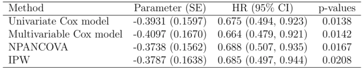
We then introduce covariate-adjusted sensitivity analysis within the established framework. For the illustrative example in the previous paper (chapter 2), we compare three methods of analysis for time-to-event data, and then we illustrate how to incorpo-rate these methods into the proposed sensitivity analysis for covariate adjustment. The three methods are the multivariable Cox proportional hazards model, non-parametric ANCOVA, and inverse probability weighting with propensity scores. The assumptions, statistical issues, and features for these methods are discussed.
Lastly we extend the underlying principle of the proposed sensitivity analysis to grouped time-to-event data. Various post-withdrawal assumptions are specified through a conditional odds ratio of failure for the discontinued vs. retained patients, so that the counts of withdrawals are redistributed to the failure counts in the following time inter-vals or to the counts censored at the end of study, as if all the withdrawers completed
follow-up. The hypothetical survival profile estimates and the inferences on treatment effects (i.e., the incidence density ratio, the odds ratio, the Mann-Whitney probability, and the Mantel-Haenszel criterion) are produced by matrix operations with the covari-ance estimators obtained using the linear Taylor’s series approximations. Therefore there is no need to perform the multiple imputation procedures for the missing out-comes (i.e., probabilistically assign the patients to a failure status in the time intervals following their withdrawals).
Acknowledgments
My most heartfelt thanks go to my mentor and co-advisor, Dr. Gary G. Koch, who coached me through my research, exposed me to scientific thinking, and allowed me the opportunity to pursue my career goals. I will be forever grateful to him for his extreme patience, generosity and encouragement.
I would like to thank my co-advisor, Dr. Amy H. Herring, for her guidance and advice, and for providing me financial assistance when I needed it the most. I also appreciate the time and effort that Drs. John S. Preisser, Benjamin R. Saville, and Haibo Zhou have devoted to my academic progress. In addition, I would like to give my special thanks to Dr. Wayne D. Rosamond for participating on my committee.
Finally, I thank all the people who have helped me during my graduate study and supported me through the completion of my dissertation, particularly Dr. Mirza W. Ali who provided some motivating background for the topic addressed by the second chapter and Dr. Suzanne Edwards who generously provided data for the illustration example in the second and third chapters.
Table of Contents
List of Tables . . . x
List of Figures . . . xii
List of Abbreviations . . . xiii
1 Literature review . . . 1
1.1 Introduction . . . 1
1.2 Withdrawal in Longitudinal Clinical Trials . . . 3
1.3 Missing Data Mechanisms . . . 4
1.4 Withdrawal Reasons in Clinical Trials . . . 8
1.5 Mixed-Effect Regression Model (MRM) . . . 9
1.6 Multiple Imputation (MI) . . . 13
1.7 Sensitivity Analysis . . . 16
1.7.1 Why Sensitivity Analysis . . . 16
1.7.2 Selection and Pattern-mixture Models . . . 18
1.8.1 Intent-to-treat and Per-protocol Analysis . . . 21
1.8.2 PM Model with Longitudinal Data via MI . . . 22
1.9 Informative Censoring and Sensitivity Analysis . . . 24
1.10 Summary . . . 26
2 Sensitivity Analyses of withdrawals in Time-to-Event Data . . . 28
2.1 Introduction . . . 28
2.2 Clinical trial examples . . . 32
2.3 Method . . . 38
2.3.1 Kaplan-Meier Multiple Imputation Strategy . . . 38
2.3.2 Parameter Estimations . . . 44
2.4 Results . . . 46
2.4.1 Performance of KMMI method underθ = 1 . . . 46
2.4.2 Sensitivity analysis . . . 53
2.5 Discussion . . . 57
3 Covariate-Adjusted Sensitivity Analysis for Time-to-event Data . . 61
3.1 Introduction . . . 61
3.2 Covariate-Adjusted Hazard Ratio Estimation . . . 65
3.2.1 Nonparametric ANCOVA . . . 65
3.2.2 Inverse probability weights using propensity score . . . 66
3.3 Sensitivity Analysis using Multiple Imputation . . . 69
3.3.1 Unadjusted multiple imputation . . . 69
3.3.2 Covariate-adjusted multiple imputation . . . 70
3.3.3 Parameter estimation . . . 71
3.4 Application . . . 72
3.4.1 Clinical trial example . . . 72
3.4.2 Covariate-adjusted analyses with MAR-like assumption . . . 76
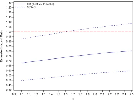
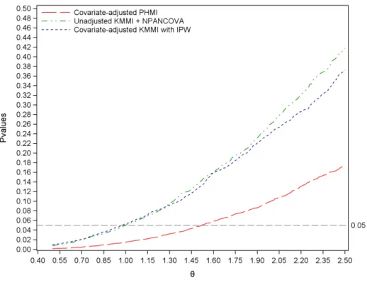
3.4.3 Sensitivity analyses with covariate adjustment . . . 81
3.5 Summary . . . 84
4 Sensitivity Analysis for Withdrawals in Grouped Time-to-event Data 88 4.1 Introduction . . . 88
4.2 Methods . . . 91
4.2.1 Data structure . . . 91
4.2.2 Survival/failure probability estimation . . . 93
4.2.3 General framework of sensitivity analysis . . . 97
4.2.4 Criteria for treatment effect comparison . . . 100
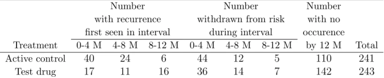
4.3 Application . . . 105
4.4 Summary and discussion . . . 116
5 Discussion . . . 118
Appendix 1: Cumulative discontinuation proportions by reasons . . . 120
Appendix 4: Conditional probability of failing (h) . . . 123
Appendix 5: Variance/covariance estimate for p . . . 128
Appendix 6: Variance/covariance estimate for hθ . . . 130
Appendix 7: Variance/covariance estimates for q and qθ . . . 132
Appendix 8: Covariance estimates for loge IDR ( ˆη) and loge OR ( ˆψ) . 137 Appendix 9: Variance estimates for Mann-Whitney probability ξ . . .ˆ 139 Appendix 10: Calculation of QM H . . . 140
Bibliography . . . 142
List of Tables
2.1 Discontinuations and the corresponding reasons by treatment groups . 33
2.2 Unadjusted and adjusted odds ratios for discontinuation . . . 36
2.3 Analyses of treatment comparisons for delaying time-to-intervention for any mood episode . . . 37
3.1 Distribution of patients’ baseline characteristics . . . 75
3.2 Association of patients’ baseline characteristics and the primary outcome (assessed with Cox model) . . . 75
3.3 Covariate-adjusted analyses for treatment effects under the MAR-like assumption . . . 77
3.4 Characteristics of the pseudo population created by standardized weights using IPW method . . . 78
3.5 Sensitivity analysis with specification of θ = 1 . . . 79 3.6 Key steps and assumptions in the performance of sensitivity analyses
under θ = 1 . . . 80 4.1 Data for endoscopic assessment in 12-month maintenance trial for
duo-denal ulcer . . . 106
4.2 Interval-specific and cumulative rate for ulcer recurrence obtained from different managements of withdrawals (i.e., crude rate, life table, and sensitivity analysis with θC =θT = 1) . . . 109 4.3 Interval-specific (loge) incidence density ratios and statistical inferences
via the linear model with design matrix X =It×t . . . 110
4.5 Common (loge) incidence density ratios and odds ratios via the linear model with design matrix X =1t . . . 112
4.6 Mann-Whitney probability and the Mantel-Haenszel criterion by differ-ent managemdiffer-ents of withdrawals . . . 112
4.7 Sensitivity analysis . . . 113
A.1 KMMI and PHMI methods with or without bootstrap resampling atθ = 1121 A.2 Alternative KMMI strategy for sensitivity analysis . . . 122
List of Figures
2.1 Cumulative discontinuation proportions by treatment groups . . . 34
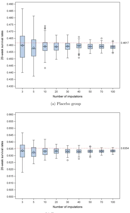
2.2 Distributions of 20 weeks survival rates for 100 replications of different numbers of imputations. The conventional KM estimates are indicated with the horizontal line. . . 48
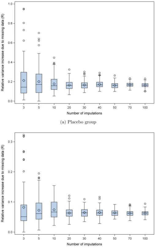
2.3 Distributions of relative variance increase due to missing data (R) of 20 weeks survival rates for 100 replications of different numbers of imputa-tions. . . 49
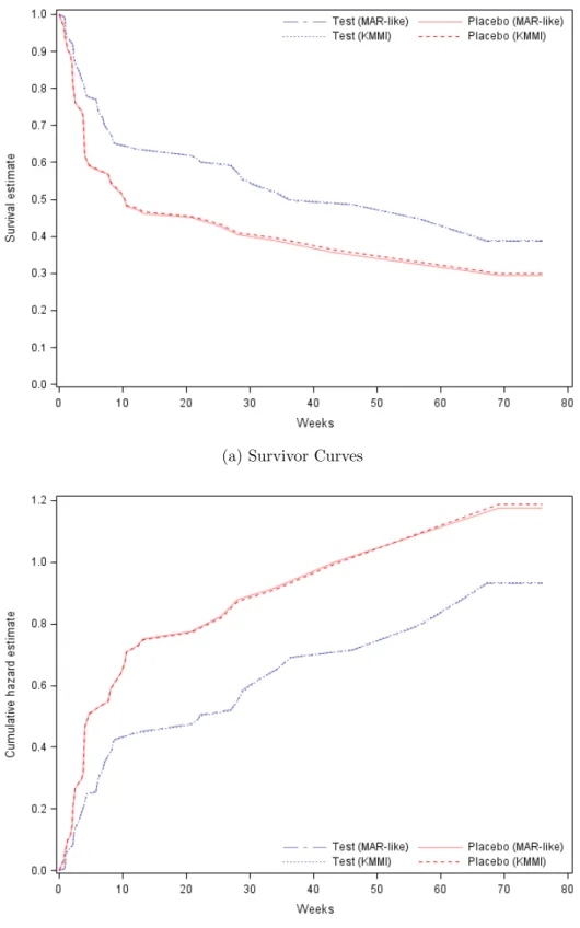
2.4 Comparison of the results from the conventional (MAR-like) and the KMMI method . . . 51
2.5 Sensitivity analysis results using KMMI method . . . 55
2.6 Sensitivity analysis results using PHMI method . . . 56
3.1 Sensitivity analyses with covariate adjustment . . . 81
4.1 Contour plots of sensitivity analysis . . . 115
List of Abbreviations
ANCOVA Analysis of covariance ANOVA Analysis of variance
GEE Generalized estimating equation
ITT Intent-to-treat
IPW Inverse probability weights
KM Kaplan-Meier
LTF Loss-to-follow-up
LOCF Last observation carried forward
MAR Missing at random
MCAR Missing completely at random
MI Multiple imputation
MNAR Missing not at random
MRM Mixed-Effect Regression Model
NPANCOVA Non-parametric ANCOVA
PM Pattern mixture
PP Per-protocol
PS Propensity score
Chapter 1
Literature review
1.1
Introduction
The efficacy of a new treatment for providing better outcome, for improving patient’s condition, or for preventing disease recurrence is typically evaluated in randomized clinical trials in which patients are followed over time. Two types of data can be collected to assess the efficacy of the new treatment: (1) Longitudinal data from the repeated measurements of a criterion on the same subject at multiple visits over time. This criterion may be a measure of functionality, physiological performance, symptoms, or general well-being. (2) Time-to-event data, where the endpoint event may be death, disease progression or recurrence.
average effect of treatment across multiple visits or the effect at the last visit could be analyzed using standard methods, such as the repeated measures mixed-effect models. For time-to-event data, the Kaplan-Meier (KM) curve, Log-rank test, and possibly the Cox proportional hazards model are most often used. However, a ubiquitous problem in all clinical trials, regardless of the outcomes, is missing data due to patients discon-tinuing study treatment before study completion. For longitudinal data, missing due to withdrawal means a patient has missing status for all visits after a certain time point. In the time-to-event analysis, it means a patient’s follow-up time is censored before the end of the study. If we are able to make the assumption of missing at random (MAR), which will be explained in the subsequent section, the usual methods men-tioned previously will provide valid analysis and interpretable results. However, one could never know for certain whether the MAR assumption is appropriate, and hence there may need to be other methods to address the robustness of conclusions about the treatment effect when departure from the MAR assumption is possible. Such analysis is sometimes calledsensitivity analysis, and it will be explained in the subsequent section. Extensive efforts have been made to establish appropriate methods for analyzing in-complete data and performing sensitivity analysis for longitudinal clinical trials. Here, we want to focus on the issue of withdrawal in the time-to-event scenario and discuss methods for sensitivity analysis for regulatory settings. Section 1.2 begins with re-viewing methods available in the longitudinal data settings, and provides the concept of withdrawal and discusses the impact of missing data in longitudinal data analyses. Section 1.3 introduces missing data mechanisms in the context of withdrawal. Section 1.4 summarizes the common reasons for withdrawal. Mixed-effect models and multiple imputation are the major analytic approaches to deal with missing data in longitudinal clinical trials; and they are described in Section 1.5 and 1.6, respectively. Section 1.7
discusses the concept and the necessity of sensitivity analysis, via selection and pat-tern mixture models. Available sensitivity analysis strategies under the intent-to-treat (ITT) principle for longitudinal clinical trials are presented in Section 1.8. Finally, the recent development of sensitivity analysis for handling dependent and informative censoring is reviewed in section 1.9.
1.2
Withdrawal in Longitudinal Clinical Trials
A defining feature of longitudinal clinical trials is that the repeated measurements on the same individual during the course of treatment allow a direct study of change in the treatment effect over time. Typically, a baseline (or pre-treatment) measurement is taken on all patients who are then randomized. Measurements of the outcome variable are then taken repeatedly at the same set of occasions for all participants in the study. At the last planned time point, the treatment difference from placebo (i.e., the efficacy of the experimental drug) can be assessed in terms of change in outcomes from baseline or average rate of change in outcomes. Although efforts are made to collect data on every individual in the trial at each time point of follow-up, some patients could stop adhering to the protocol or discontinue their study treatment for reasons beyond the control of investigators. Consequently, the subsequent follow-up data will be missing (i.e., monotonic missing). If a patient is no longer seen after a certain follow-up visit, we say the data is missing due to withdrawal. In the literature, dropout and loss to
follow-up are also used synonymously.
analysis methods may lead to conflicting statistical inferences about treatment ben-efit (Permutt and Pinheiro, 2009). Furthermore, incorrectly addressing missing data may bias parameter estimates, inflate Type I and Type II error rates, and degrade the performance of confidence intervals, thereby leading to incorrect conclusions about treatment effect (Collins et al., 2001).
1.3
Missing Data Mechanisms
To understand how statistical inferences may be affected by missing data, it is important to understand the missingness mechanisms. The following terminology is based on the standard missing data framework of Little and Rubin (2002).
In the context of a longitudinal clinical trial, we assume that k measurements are to be obtained at times t1, ..., tk for n independent subjects. For subject i, i= 1, ..., n, a set of measurements yij (j = 1, ..., k) is collected, and we define the following:
• yi = (yi1, ..., yik) is a (1× k) complete data vector of outcomes for subject i, possibly with monotonic missing data.
• ri is the missing data indicator. Specifically, letrij = 1 if yij is observed; and let
rij = 0 if yij is missing.
• Givenri,yi can be partitioned into (yio, y m
i ), corresponding to the observed and
the missing part of yi.
Then, the full data density can be factored into two parts as follows:
f(yio, yim,ri|Xi,θ,ψ) = f(yoi, yim|Xi,θ)f(ri|yio, ymi , Xi,ψ). (1.1)
Here, Xi is the design matrix for observed covariates, and θ and ψ denote parameter vectors for the measurement and missingness mechanism, respectively. The first factor
is the marginal density of the measurement process, and the second one is the density of the missingness process conditional on the outcomes.
Under a missing completely at random (MCAR) mechanism, the missingness is assumed to be unrelated to either the observed data or the missing outcomes, i.e.,
f(ri|yio, y m
i , Xi,ψ) = f(ri|ψ). (1.2)
Therefore, 1.1 simplifies to
f(yio, ymi ,ri|Xi,θ,ψ) =f(yio, ymi |Xi,θ)f(ri|ψ), (1.3)
indicating the independence of the measurement and missingness mechanisms. The joint distribution ofyo
i and ri becomes
f(yio,ri|Xi,θ,ψ) =f(yio|Xi,θ)f(ri|ψ). (1.4)
Hence, in whatever way the observed data are analyzed (whether using a frequentist or likelihood method), the missingness mechanism is ignorable. For instance, under MCAR, analysis restricted to cases for which all measurements were recorded (i.e., a complete-case analysis) will yield unbiased estimates. Furthermore, MCAR also im-plies that the distribution of unobserved outcomes after withdrawal is the same for those who do and do not withdraw, and the outcomes for those who withdraw has the same distribution as the target population (Fitzmaurice, 2003). Unfortunately, those assumptions are often not realistic.
Under a missing at random (MAR) mechanism,ri depends on yi only through its
observed part yo
and yio), the missingness is independent of the missing outcomes:
f(ri|yoi, yim, Xi,ψ) =f(ri|yio, Xi,ψ). (1.5)
The full data density is partitioned as
f(yoi, yim,ri|Xi,θ,ψ) = f(yoi, yim|Xi,θ)f(ri|yio, Xi,ψ). (1.6)
At the level of observed data, we obtain
f(yio,ri|Xi,θ,ψ) =
Z
f(yio, yim|Xi,θ)f(ri|yio, Xi,ψ)dyim (1.7) =f(yio|Xi,θ)f(ri|yio, Xi,ψ).
Ifθ and ψ are disjoint, then the likelihood can be factorized into two distinct compo-nents. The missingness isignorable within the likelihood framework, and inference can be based solely on the marginal density of the observed data,f(yo
i|Xi,θ). Apparently,
under the MAR process, the distribution of the outcomes for those who withdraw is not the same as the distribution in population. But conditional on the observed out-comes prior to the withdrawal occasion, the distribution of the unobserved outout-comes following withdrawal is the same for those who do and do not withdraw at that oc-casion. However, this aspect of the assumption cannot be tested from the data at hand (Fitzmaurice, 2003).
Covariate-dependent missing is a special situation, where the missingness only de-pends on the fixed covariatesXi, but not on the outcomes yi, that is,
f(ri|yio, yim, Xi,ψ) = f(ri|Xi,ψ). (1.8)
Molenberghs and Kenward (2007) viewed it as a special case of MCAR. But Little (1995) suggested the term ‘MCAR’ should be reserved for the case where the missingness dose not depend on either yi or Xi, as shown in (1.2). When the missingness mechanism is only associated with the observed data (MAR), conditional on the fully observed data regardless of either the fixed covairatesXi or the observed outcomesyi, the
miss-ingness is completely at random (MCAR). Hence, it is reasonable to refer assumption (1.8) as ‘covariate-dependent MAR’ and refer assumption (1.5) as ‘outcome-dependent MAR’ (DeSouza et al., 2009).
Finally, when a missing not at random (MNAR) mechanism operates, the miss-ingness depends on the unobserved outcomes ym
i , perhaps in addition to y o
i. The
joint distribution of yi and ri (1.1) cannot be further simplified. Conditional on the
past outcomes prior to the withdrawal occasion, the distribution of the future out-comes following withdrawal is different for those who do and do not withdraw. Clearly, the missingness mechanism is non-ignorable, and the distribution of the unobserved outcomes for those who withdraw is not estimable from the data on those observed after withdrawal. Therefore, the inference can only be made by the joint models of measurement and missingness processes, with model assumptions about missing data mechanism. Such models can be formulated in either theselection model or the
pattern-mixture model framework. For selection models, the full data density is factored as the
marginal density of the measurement process and the density of the missingness pro-cess, conditional on the outcomes (as shown in 1.1). While the pattern-mixture models use the reverse factorization,
f(yoi, yim,ri|Xi,θ,ψ) = f(yio, yim|ri, Xi,θ)f(ri|Xi,ψ), (1.9)
allowing a different response model for each pattern of the missing value.
of θ and ψ are often called ignorable, because unbiased estimates of parameters can be obtained from observed data. The same requirement hold for Bayesian inference. But for non-likelihood frequentist inference, such as analysis of variance (ANOVA) and generalized estimating equation (GEE) method, MCAR is the only sufficient condition for ignorability. Either MNAR or MAR with parameters in common is called
non-ignorable. When missingness is non-ignorable, the inference based on the likelihood
ignoring the missingness process is biased (Molenberghs and Kenward, 2007).
1.4
Withdrawal Reasons in Clinical Trials
In general, no statistical test is available to assess from which mechanism the missing data arise. Hence, in longitudinal clinical trials, an intuitive way to explore missingness is to look at the reasons for withdrawals. Siddiqui et al. (2009) summarized the common reasons as follows: (i) recovery, (ii) lack of improvement, (iii) treatment-related side-effects, (iv) unpleasant study procedure, (v) intercurrent health problems, and (vi) external factors unrelated to the trials. For example, MCAR might result from a patient dropping out because of relocation (vi). If a patient was observed doing poorly and then decided to discontinue participation, then the withdrawal was related to the outcome of interest and was explained by the observed data. In this case, it is reasonable to assume MAR. An example of MNAR could be an instance in which a patient had been doing well and was then lost to follow-up due to a worsened condition after the last observed visit (Mallinckrodt et al., 2003).
However, so far, there is no formal classification of withdrawal reasons into the three missingness mechanisms defined by Little and Rubin (2002). This might partially be due to the fact that the definition of missingness mechanisms is based on the relation-ship between outcome and independent variables, and this relationrelation-ship could vary from case to case (Siddiqui et al., 2009). For instance, withdrawals due to adverse events
are probably not MNAR in many cases because all the relevant data probably were ob-served. But whether classifying it as MCAR or MAR depends on the specific situation. In many clinical trial settings, extensive efforts are made to observe all the possible out-comes and the factors that influence withdrawal. Thus, the MAR assumption is much more plausible than the MCAR assumption, because the observed data could explain much of the missingness in many scenarios (Mallinckrodt et al., 2003). In principle, clinical trials by their very design seek to minimize the amount of MNAR. But, the possibility of MNAR can never be ruled out, and a mixture of different missingness mechanisms in a clinical dataset often takes place.
Within the framework of pattern mixture models, we develop sensitivity analy-sis methods for time-to-event data with possibly informative censoring. The chapter 2 presents a multiple imputation (MI) method for sensitivity analysis of continuous time-to-event data, invoking multiple imputation of the missing failure times due to withdrawals. In the chapter 3, we discuss the covariate-adjusted sensitivity analysis within the established framework. In the chapter 4, the underlying principle for this type of sensitivity analysis is extended to grouped time-to-event data.
1.5
Mixed-Effect Regression Model (MRM)
The linear mixed models assume that the vector Yi of k repeated continuous
mea-surements for theith subject satisfies
Yi|bi ∼N(Xiβ+Zibi,Σi) (1.10)
bi ∼N(0, G)
where β is the p-dimensional vector of fixed effects; bi is the q-dimensional vector of
subject-specific random effects; and Xi(k ×p) and Zi(k ×q) are the corresponding design matrices. It then can be easily derived that, marginally,
Yi ∼N(Xiβ, Vi) and Vi =ZiGZi0+ Σi. (1.11)
Conditional onbi, the outcomesYij’s,j = 1,2, ..., k, are usually assumed to be mutually independent. In this case, model residuals are uncorrelated, that is, Σi =σ2Ik×k.
The generalized linear mixed models combine generalized linear model concepts with ideas from linear mixed models. It is assumed that, the conditional distributions of outcomes Yij’, givenbi, are independent, and in the form of the exponential-family
fi(yij|bi,β, φ) = exp{φ−1[yijθij −ψ(θij)] +c(yij, φ)}
bi ∼ N(0,G)
with
η(µij) = η(E(Yij|bi)) =x0ijβ+z0ijbi
for a known link function η(·), where φ is a scale parameter, andθij is the canonoical parameter and satisfies dψ(θij)/dθij=E(Yij|bi)=µij. Unlike linear mixed models, the marginal likelihood of the generalized linear model often involves the approximation of integration over theq-dimensional random effects. This is because, in most situations,
the integrals can not be solved analytically.
Typically, clinical trials are conducted to assess the fixed effects (i.e. the difference in treatment effects), rather than the subject-specific random effects. To accommodate this focus, the marginal linear mixed model (1.11) is often implemented in analyzing the continuous outcome measures with pre-specified time points. In this formulation, the random effects are modeled as a part of the marginal covariance matrix V, and the fixed effects could include treatment effect, time trend, treatment-by-time inter-action and other covariates, such as baseline measurement or risk factors. Mallinck-rodt et al. (2008) referred to this model as mixed-effects model for repeated-measures analysis (MMRM). A common implementation of MMRM is a cell mean model with unstructured within-subject error covariance structure V. More specifically, the out-come measure on the ith patient with treatment t at the jth occasion is modeled as
yijt =µjt+εij, whereµjt is the group mean of treatment t at the jth occasion and εij is thejth element of the residual vectorεi withεi ∼N(0, V). This version of MMRM
is well suited to the general characteristics of clinical trials, i.e., common scheduled measurements for all patients and relatively a small number of measurement occasions. In addition, the unstructured covariance modeling relaxes the assumption about within patient correlation and often provides the best fit to the data.
broadly speaking, MMRM analysis, as well as other MAR model-based methods, could be considered as a per-protocol(PP) analysis for the intent-to-treat(ITT) population.
Also, the MMRM analysis can be easily implemented using standard software, such as the SAS Procedure Mixed (SAS Institute, Cary, NC). A series of simulation studies have been conducted to compare the performance of MMRM with last observation carried forward (LOCF), in evaluating treatment efficacy under different missing data mechanisms (Mallinckrodt et al., 2008; Siddiqui et al., 2009). LOCF is an ad hoc method commonly used to impute missing values due to withdrawal for the primary efficacy analysis of clinical trials. Under MCAR or MAR, the MMRM analysis was able to estimate the true treatment difference with a negligible bias and control the type I error rate at a nominal level, whereas LOCF underestimated the standard error, and yielded increased bias and inflated type I error. Furthermore, in the presence of MNAR mechanism or a mixture of the three missing mechanisms, the MMRM analysis was also superior to LOCF in minimizing estimation bias and controlling type I and II error rates. In general, it has been recognized that the likelihood based MMRM is a robust and appropriate approach to handle missing data for primary efficacy analysis. However, a shortcoming for MMRM and almost every model-based approach is that ignorable missingness depends on correct model spiflication. Missingness that might be non-ignorable given one model could be ignorable given another (Mallinckrodt et al., 2008). For instance, if withdrawal depends only on an observed variable, say treatment, and treatment is included in the analytic model, then the mechanism giving rise to the withdrawal would be ignorable (MCAR), and statistical analysis results would be unbiased. Whereas if treatment is not included in the analytic model, the missingness mechanism would be non-ignorable (MNAR), consequently the inference based on such a model would be biased.
1.6
Multiple Imputation (MI)
Multiple imputation was first introduced by Rubin (1987) to handle missing re-sponses in a sample survey. Under ignorable missingness, it is another feasible approach for analyzing incomplete data. Three steps are involved in MI analysis:
1. The missing values (ym) are filled M times by an imputation model to generate M
complete data sets. Each value is a random draw from the conditional distribution of the missing value given the observed data, in such a way that the imputations properly represent the information about the missing value in the imputation model.
2. Each of the M complete data sets is then analyzed using the method that would have been appropriate if the data had been complete (i.e., the analysis model).
3. The estimates of the desired quantities and associated standard errors from sep-arate M analyses are combined into a single inference .
The MAR assumption needs to apply only for the first step, which can be carried out by the SAS procedure MI. The statistical inference performed in the second step will be valid, if the missingness given the imputation model is ignorable. The third step could be conducted by the SAS procedure MIANALYZE using the multiple imputation technology given by Rubin (1987).
More specifically, suppose thatθ is the parameter of interest to be estimated using a analysis model. If complete data were available, the inference about θ given large samples would typically be based on the point estimate ˆθ(yo, ym), the variance estimate
ˆ
Vθ(yo, ym), and the appropriate normal approximation (ˆθ−θ)
p
Let ˆθm and Vm denote the point and variance estimates from the mth imputed data set (m = 1,2, ..., M). The MI estimate for θ is simply the average of estimates from the M imputed complete data sets,
¯
θ= 1
M
M
X
m=1
ˆ
θm. (1.13)
Also, defineW = M1 PM
m=1Vm to be the average of theM within-imputation variances,
and B = M1−1PM
m=1(ˆθ
m − θ¯)2 to be the between-imputation variance. Then, the
variance estimator of ¯θ is given by the sum of W and B multiplied by a finite sample correction,
V =W + M+ 1
M B. (1.14)
Confidence interval estimates and hypothesis tests are based on the approximation of at distribution
V−12(¯θ−θ)∼t
ν (1.15)
with degrees of freedom ν = (M −1)(1 +r−1)2, where r = (1 +M−1)B/W. Thus, a 100(1−α)% confidence interval estimate forθis ¯θ±tν,(1−α
2)V 1
2; and a two-sidedp-value
for the null hypothesisH0 :θ = 0 is obtained by comparing ¯θ/V
1
2 with the distribution
of tν.
Notice that if ym carried no information about θ, the imputed data estimates ˆθm would be identical andV would reduced to W. Therefore, r, the ratio of the between-imputation to the within-between-imputation variation, measures the relative increase in vari-ance due to missing information. When there is no missing information about θ the values of r and B are both zero. The rate of missing information in the system can be
obtained by comparing the spread of the distribution in (1.12) to the distribution in (1.15) as
γ = r+ 2/(ν+ 3)
1 +r . (1.16)
Unlike maximum likelihood (ML) based mixed-effect models, the MI approach han-dles missing data in a imputation step entirely separate from the analysis. The model used to impute missing values can differ from the model used for inference (Liu and Gould, 2002). An advantage about the MI method, compared to the ML mixed-effect model approach, is that the imputation model can include considerably more variables predictive of missingness, therefore increasing the plausibility of the MAR assump-tion (Mallinckrodt et al., 2003). Besides the variables that are potential causes or correlates of the missingness itself, the imputation model could also include the vari-ables that are simply correlated with the varivari-ables that have missing values regardless of their relation to the missingness mechanism. Collins and colleagues referred to this class of variables as auxiliary variables (Collins et al., 2001). Their simulation study indicated that incorporating the auxiliary variables not only increased efficiency and statistical power under MAR, but also reduced the bias and moved the situation closer to MAR when missingnes was non-ignorable. In clinical trial settings, the auxiliary variables, such as postbaseline or time varying covariates correlated with treatment could be included in the imputation model. But those variables cannot be included in the analysis model or the MMRM model because of their confounding with the treatment effect (Mallinckrodt et al., 2008).
do not facilitate the use of auxiliary variables. Using MI, it is much easier to incor-porate auxiliary variables into the analysis via the imputation step. For this reason, the MI method is practically more robust against misspecification of the missingness mechanism than the direct likelihood method.
1.7
Sensitivity Analysis
1.7.1
Why Sensitivity Analysis
When analyzing incomplete data, additional assumptions about missing data have to be made in order to choose sensible statistical methods. Those assumptions break down into two broad categories as follows (Carpenter and Kenward, 2008). The first type of assumptions focuses on the missingness mechanism, specifically, how the probability of missingness depends on the observed and unobserved data. This leads to the selection model approach. The second type of assumptions focuses on the distribution of missing data given the observed data, that is, whether or how the distribution of unobserved outcomes is different from the distribution of outcomes for those who have no missing data, and how this difference depends on the patterns of the missingness. This is the extension of pattern mixture models. In section 1.3, the connections between the missingness mechanisms and the assumptions of missing data distribution were discussed in the context of MCAR, MAR, and MNAR.
Depending on the statistical approach we adopt to handle the missing data, we need to make assumptions about either the missingness mechanism or the missing data dis-tribution. Unfortunately, neither of those assumptions can be validated definitely from the observed data. For instance, MCAR indicates the distribution of outcomes prior to withdrawal is the same for those who do and do not withdraw at that occasion, which can be suggested by the observed data. But we cannot be completely sure that data
are MCAR, since we do not observe the missing outcomes. Nevertheless, the observed data can rule out MCAR, if there is any relationship between the observed data and the occurrence of missing data (Carpenter and Kenward, 2008). In clinical trials, MCAR is most unlikely, and MAR is often reasonable; however, the possibility of MNAR is impossible to be ruled out. Results from likelihood-based MAR methods without con-sideration of their limitations could be misleading (Mallinckrodt et al., 2003). Thus, In many circumstances, analysis valid under MNAR assumption is required. However, one obvious and fundamental problem is that the conclusion of the MNAR analysis is conditional on the appropriateness of the assumed model (Mallinckrodt and Ken-ward, 2009), and MNAR model assumptions are not verifiable from the observed data. More importantly, the consequences of model miss-specification are more severe with MNAR methods than with MAR methods. Hence, no single MNAR approach can be considered definitive or well suited for the primary analysis in confirmatory clinical trials.
Given the above discussion, no universally best applicable approach for handling missing data can be recommended. Investigators should make effort in exploring the impact of missing data assumptions on the results of analysis. For longitudinal clinical trial data, it has been a broad consensus among statisticians in the pharmaceutical industry and academia that likelihood-based methods implemented under the MAR framework are the sensible choice for the primary analysis, and a series of MNAR analyses should be implemented as sensitivity analysis to assess the robustness of the primary analysis result to the possible departure from the MAR assumption (Mallinck-rodt and Kenward, 2009).
conclusions (Molenberghs, 2009). In clinical trial settings where interest is in the treat-ment efficacy hypothesis, a pre-defined sensitivity analysis approach was recommended by Carpenter and Kenward (2008) as follows. Either before the trial is conducted, or during a blind review of the data, investigators identify a set of missing data mod-els (i.e., assumptions about missingness mechanism or missing data distribution) to address the impact of clinically plausible departure from MAR. A sensible analysis is then planned under each missing data model. After the blinding is broken, a series of analyses are performed. The results from such analyses would reflect a range of conclusions under assumed models, and therefore demonstrate the robustness of the inference about treatment comparisons to different missing data assumptions.
1.7.2
Selection and Pattern-mixture Models
The sensitivity of inference to missing data assumptions is typically investigated via selection or pattern-mixture models under MNAR framework. Carpenter and Kenward (2008) illustrated the application of both approaches using clinical trial examples.
Selection models (Diggle and Kenward, 1994; Little and Rubin, 2002) describe the full data likelihood as the product of the marginal density of the measurement process and the density of the missingness process conditional on outcomes (shown in 1.1). Besides the model for the measurement process as used in MAR analysis, a model explaining missingness has to be fitted at the same time in the analysis. Carpenter and Kenward (2008) gave an example of the missingness process model for withdrawal as
logitPr(Rij = 0|Ri(j−1) = 1) =αj+δYij (1.17) Pr(Rij = 0|Ri(j−1) = 0) = 1,
whereYij denotes the response of interest for theith subject at thejth visit,i= 1, ..., n
and j = 1,2, ..., k. Here, the log odds of subject i withdrawal at the jth visit depends not only on that visit (αj), but also on the response at that visit. δ = 0 corresponds to a MAR assumption, and a positive value of δ implies odds of withdrawal at a visit increases with the value of response at that visit. Using MCMC methods in winBUGS (Spiegelhalter et al.,1999), this model can be fitted in conjunction with a mixed model for the measurement process. However, the estimated value of δ and its standard error depend critically on unverifiable assumptions for the missing data distribution. Thus, estimating δ is usually not recommended (Carpenter and Kenward, 2008). Rather, in-vestigators should identify a set of plausible values for δ, then fit the model with each of these values, and explore how the estimated treatment effect varies as a sensitiv-ity analysis. In many applications, model (1.17) could be extended to include other variables, such as, treatment and response from previous visit. Theoretically, variables that are included in a mixed model to maximize the plausibility of MAR should be included to make the selection model more plausible and make the treatment estimates less sensitive to MNAR. However, those complicated models are sometimes difficult to fit and interpret.
analytical models are fitted separately for different groups, defined by withdrawal pat-terns (e.g. early or late withdrawals, and completers), and then the overall estimate is obtained as a weighted average of the pattern-specific estimates (Siddiqui et al., 2009; Ali and Siddiqui, 2000).
A natural way to perform sensitivity analysis under the PM framework is to assume that the model for missing data is a modification of the model for observed data. By varying this modification, a range of sensitivity analyses could be easily performed. Carpenter and Kenward (2008) illustrated this type of sensitivity analysis using an example with a single response from normal distribution. For the control arm, assume that the observed responses come from normal(µC, σ2) and the unobserved responses have shifted mean (µC +δC). Let πC denote the probability of withdrawal, then the average response in the control arm is (1−πC)µC +πC(µC +δC). Likewise, for the intervention arm, µI, δI, and πI are defined analogously, then the average response in the intervention arm is (1−πI)µI+πI(µI+δI). The averaged treatment effect, ∆, is then
∆ = ((1−πI)µI+πI(µI+δI))−((1−πC)µC +πC(µC+δC)) (1.18) = (µI−µC) + (δIπI−δCπC).
Note that (µI−µC) is the treatment effect in completers,δI and δC are the parameters describing the degree of informative missingness, and δI = δC = 0 implies MCAR. Using a Bayesian approach, the sensitivity analysis could be performed via a series of plausible prior elicitation about the joint distribution of δI and δC.
1.8
Intent-to-treat Analysis and Sensitivity Analysis
1.8.1
Intent-to-treat and Per-protocol Analysis
Intent-to-treat(ITT) has been accepted as a fundamental principle for establishing efficacy/effectvieness in randomized confirmatory clinical trials. ITT analysis attempts to evaluate the effect of the original treatment strategy rather than directly assess the effect of treatment itself (Flyer and Hirman, 2009). It includes all randomized patients, regardless of adherence to the protocol or premature withdrawal. In a typical ITT analysis, the treatment effect is measured with patients assigned to the treatment as randomized, rather that to the treatment actually received (Little and Yau, 1996).
In contrast to ITT analysis, per-protocol (PP) analysis incorporates actual treat-ment usage and compliance into a direct measuretreat-ment of treattreat-ment effect. In the pres-ence of missing data due to withdrawals, PP analysis seeks to estimate the treatment effect that would have been seen if all patients completed their assigned treatment. In this regard, PP analysis is consistent with the MAR assumption, under which the missing data problem in longitudinal data can be properly addressed by ML based mixed-effect models (Carpenter and Kenward, 2008; Flyer and Hirman, 2009).
treatment. Very often, when patients stop complying with the protocol, they withdraw from the study, leading to missing responses.
1.8.2
PM Model with Longitudinal Data via MI
Because of the distinction in the underlying hypothesis between ITT and PP anal-yses, methods to address the missing data issue for ITT analysis should be different correspondingly from those for PP analysis. We should consider that the distribution of responses is different for those who do and do not continue with the intervention protocol, and even after taking into account the information in observed data, the withdrawal mechanism may still depend on the unseen response (Carpenter and Ken-ward, 2008). Furthermore, if the withdrawal is likely to be associated with a change in treatment regime, then a different model is needed for those who withdraw. However, we may not actually have enough information to model patients’ treatment adher-ences and behaviors following withdrawal. Therefore, the missing data issue following withdrawal in the ITT setting should be viewed as a MNAR analysis under specific assumptions (Carpenter and Kenward, 2008).
Under MNAR, a range of missingness process models could be consistent with the observed data. Thus, there is no longer a definitive ITT analysis (Carpenter and Kenward, 2008). Different post-withdrawal behaviors should be incorporated into sen-sitivity analyses as part of the ITT analysis. A natural approach for such a sensen-sitivity analysis is multiple imputation using PM models conditional on all relevant observed data and different missing patterns to reflect treatment change (or discontinuation) after dropout. Little and Yau (1996) proposed a PM imputation model including the treatment dosage actually received after withdrawal, upon which multiple imputations were created by sequential Bayesian draws from the parameter posterior distribution and the missing value predictive distribution conditional on the drawn parameters. The
sensitivity analysis was then carried out for a range of plausible alternative assumptions about dosage after withdrawal. A key feature of this method is that the imputation model differs from the model used for ITT analysis. Under the ITT principle, the anal-ysis model must not include compliance information following randomization, but the imputation model has no problem to incorporate such compliance information (Car-penter and Kenward, 2008).
treatment comparison estimates (Carpenter and Kenward, 2008).
1.9
Informative Censoring and Sensitivity Analysis
Survival analysis is used in medical research for analyzing time-to-event (survival) data, which is the time duration from a well-defined time origin to the occurrence of a particular event. A distinguishing feature of time-to-event data is that they are usually censored or incomplete in some way. The survival time is said to be (right) censored if the observation period was cut off before the event occurred. In such case, we do not know when (or, indeed, whether) the patient will experience an event, and we only know that the patient has not had the event at the last observed time.
In a typical setting for analyzing censored survival data, there is a potential censor time C and a potential survival time T for each individual. We only observe time
Y= min(T, C) and the censor indicator δ = I(T ≤ C), which indicates whether a failure is observed. Under this condition, the distribution ofT is not identifiable unless we make further assumptions. An important assumption in most survival analysis is that the censoring mechanism is non-informative or ignorable. This means that the instantaneous failure rate given subject survival to timet is not changed by additional information that the subject was uncensored up to that time t (Leung et al., 1997; Lagakos, 1979). In another words, the censoring of an observation does not provide any information regarding the prospect of survival time of that particular subject beyond the censor time. The contribution of a censored observation to the likelihood is just the probability that survival time T exceeds the censor time c. Therefore, the censoring mechanism is irrelevant for inference about the distribution ofT.
In general, censoring due to study termination is called end-of-study or administra-tive censoring, as apposed to loss-to-follow-up (LTF) censoring when patients withdraw during the study period (Leung et al., 1997). It is usually reasonable to assume that the
administrative censoring is independent of the survival time. Lagakos (1979) proved that independent censoring is a special case of the noninformative censoring; hence the administrative censoring imposes no problem to the standard survival analysis proce-dures. However, it is not always proper to make non-informative assumptions about the loss-to-follow-up censoring. When the probability of censoring depends on the sur-vival time, the censoring mechanism is said to beinformative (Kalbfleisch and Prentice, 2002), and the inference based on the standard methodologies is no longer valid (Col-lett, 2003). If patients who withdraw are at higher risk of subsequently having an event (i.e., the survival time and the censor time are positively correlated), the Kaplan-Meier estimator would overestimate the survival function of T. Similarly, if the withdrawals are at lower risk of failure (i.e., the survival time and the censor time are negatively correlated), then the survival function would be underestimated (Leung et al., 1997). Consequently, the main issue, related to the informative censoring in clinical trials, is the potential bias in comparison of survival functions between treatment groups.
make the problem identifiable. Scharfstein and Robins (2002) proposed classes of semi-parametric models for the cause-specific hazard of censoring indexed by censoring bias functions. Their method allows adjustment for informative censoring due to measured prognostic factors for failure time, and simultaneously quantifies the sensitivity of the inference to residual dependence between failure and censoring due to unmeasured factors. Siannis et al. (2005) studied the sensitivity analysis for informative censoring in parametric survival models. The association betweenT and C was modeled by the conditional distribution ofC given the (possibly unobserved)T through a bias function and a dependence parameter. The sensitivity analysis was developed on a range of the dependence parameters for small values. Recently, Ruan and Gray (2008) investigated the effect of the dependence between dependent withdrawal and disease progression time using a conditional probability model incorporating a set of sensitivity parameters. They linked the sensitivity analysis to the log-rank test via constructing log-rank-type score statistics from the estimated distributions, and they explored the impact of the sensitivity parameters on the inference by examining how much dependence between the disease progression and withdrawal times would need to be present to ultimately change the conclusion from the statistic for inference about the comparison of two treatment groups.
1.10
Summary
Within the framework of pattern mixture models, we develop sensitivity analy-sis methods for time-to-event data with possibly informative censoring. The chapter 2 presents a multiple imputation (MI) method for sensitivity analysis of continuous time-to-event data, invoking multiple imputation of the missing failure times due to withdrawals. In the chapter 3, we discuss the covariate-adjusted sensitivity analysis within the established framework. In the chapter 4, the underlying principle for this
Chapter 2
Sensitivity Analyses of withdrawals
in Time-to-Event Data
2.1
Introduction
treatment (Flyer and Hirman, 2009). For example, the comparison of regimens that begin with test treatment or placebo followed by effective rescue therapy after their discontinuation could erroneously suggest that an ineffective test treatment is effective solely because it forces more patients to switch to rescue therapy than placebo (Per-mutt and Pinheiro, 2009). Thus, in such situations, analyses for the comparison of the assigned treatments may need to ignore any unclear information subsequent to their discontinuation and thereby proceed with the corresponding experiences of patients as if missing.
Analytical strategies for drawing inferences from incomplete data rely on untestable assumptions about the missing data distributions and the missingness mechanism (NRC, 2010; CHMP, 2010). Little and Rubin (2002) classified the missing data mechanism into three categories: missing completely at random (MCAR), missing at random (MAR), and missing not at random (MNAR). When the data are MCAR, the missing data are unrelated to the observed and unobserved study variables, and so the observed data are statistically representative for the experiences of all randomized patients. In practice, however, MCAR is usually an unrealistic assumption. When the data are MAR, the missingness depends only upon the observed study variables. That is, conditional on the observed study variables, the probability of missing does not depend on the values of the missing data. When the missingness probability also depends on the values of the missing data, the data are said to be MNAR. In many situations, the MAR paradigm is realistic for the primary analysis in confirmatory clinical trials (Zhang, 2009; Mallinck-rodt et al., 2008). However, the observed data can never rule out the possibility of MNAR. Therefore, sensitivity analyses exploring the implications of departures from the primary MAR assumption are always of interest to assess the robustness of the treatment effect inferences.
Conventional methods such as the Kaplan-Meier estimation of survival curves (Kaplan and Meier, 1958), the logrank or Wilcoxon tests (Mantel, 1966; Gehan, 1965), and the Cox proportional hazards model (Cox, 1972) are frequently employed to describe time-to-event distributions and to assess treatment effects. Missing data for a time-time-to-event occurs for patients who prematurely discontinue follow-up for the assigned treatment (or the study) prior to the occurrence of the event or the end of their planned follow-up period (or the administrative closing date of the study). One way to address this type of missing data is to censor the follow-up times of such patients at their times of premature discontinuation. Such censoring is non-informative in a sense like the MAR assumption (Heitjan, 1994) when the assumption of its independence from the possibly unobserved time-to-event applies; i.e., the possibly unknown true time to the event for a patient is the same regardless of whether or not it is actually observed (or whether censoring occurs or not prior to it). Unfortunately, the conventional MAR-like methods ignore the fact that the patients who discontinue the assigned treatment no longer receive it after discontinuation. Instead, they attempt to estimate what would be expected for the study if all patients remained on their assigned treatments until the occurrence of the event or the end of their planned follow-up period (Flyer, 2009). Alternatively, discontinuation from treatment can be specified as clinical failure when the event of interest is unfavorable (Flyer and Hirman, 2009). In this case, one has a composite endpoint (i.e., time to the event of interest or discontinuation), and it expresses the time period for which a patient has had favorable experience with treatment. The application of this method to both the control and the test treatment groups produces what can be called the worst-case analysis, because patients who dis-continue treatment are managed as having much higher risk of a future event than other patients (Rothmann et al., 2009). In contrast, the method in which a control patient who discontinues treatment has their follow-up time censored at the time of
discontinuation and such a test treatment patient is managed as having the event is known as a worst-comparison analysis (Rothmann et al., 2009). The result from the worst-comparison analysis provides a stringent boundary on the impact of patients who discontinued treatment. Both the worst-case analysis and the worst-comparison anal-ysis have potentially unclear relevance for a study because they both make unrealistic assumptions (Wittes, 2009). Usually, they are not designated as the primary analysis, but they can be used as sensitivity analyses with the worst-comparison analysis invok-ing maximal stress to the robustness of the study results (Walton, 2009). If the study conclusions are not altered by such methods, then one is reassured regarding the va-lidity of the primary MAR-like analysis. Nevertheless, many studies will not maintain robustness to such sensitivity analyses. Hence, these methods are often criticized as unrealistically stringent and potentially problematic for a promising therapy to show effectiveness (Yan et al., 2009).
can then be analyzed by the standard methods for right censored time-to-event data. A key feature of this multiple imputation method for sensitivity analyses is a corre-sponding hazard ratio parameter θ for how the conditional survival distribution for the missing extent of follow-up can allow for different post-discontinuation behaviors of patients from the placebo and the test treatment groups. One can then investigate the impact of departures from the primary missingness assumption (i.e., non-informative independent censoring) by summarizing the treatment effect as a function of θ over a plausible range. This multiple imputation method is an extension and modification of the work by Taylor et al. (2002), where the conditional KM estimators were used to impute failure times for survival analyses under a specification for non-informative censoring. The implementation of this method is illustrated with data from a clinical trial in psychiatry.
2.2
Clinical trial examples
For illustrative purposes, we consider time-to-event data based on a clinical trial pertaining to maintenance treatment for bipolar disorder (Calabrese et al., 2003). For reasons related to the confidentiality of the data from this clinical trial, the example in this paper is based on a random sample (with replacement) of 150 patients with the test treatment and 150 patients with placebo. The study design for this clinical trial had an 8 to 16 weeks run-in period within which all patients received test treatment. Eligible patients who tolerated and adhered to this therapy were randomized to the test treatment or to the placebo, and then followed for up to 76 weeks as the planned follow-up period. Accordingly, this study had a randomized withdrawal design, and the primary efficacy endpoint was the time-to-intervention for any mood episode.
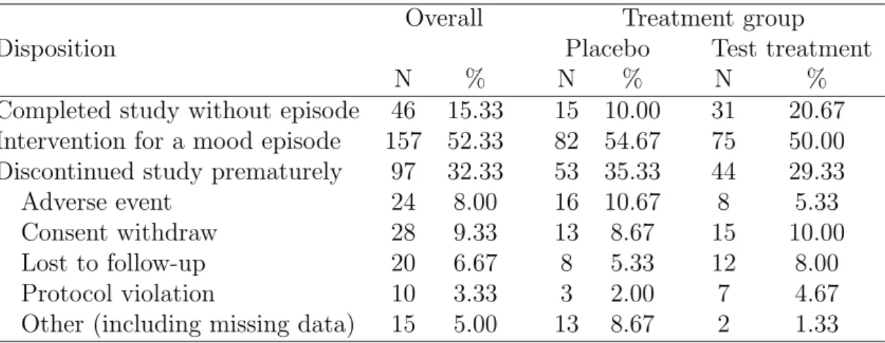
A total of 97 (32.33%) patients discontinued the study prematurely (35% on placebo and 29% on test treatment). Cumulative proportions of discontinued patients are shown
in Figure 2.1 (which has the convention of managing the patients who completed the study with the primary event as having imputed follow-up of 76 weeks without pre-mature discontinuation). Discontinuations predominantly occurred before 35 weeks with higher cumulative proportions for the placebo group. The documented reasons for discontinuation are summarized in Table 2.1, although except perhaps for ”adverse events”, they are not informative about possible missing data mechanisms. The cumu-lative proportions of discontinuation by those reasons are displayed for each treatment arm in Figure A.1 of the Appendix. For an informal evaluation of the association of discontinuation with treatments, patients’ demographics, and baseline psychiatric as-sessments, we used logistic regression models for the odds of discontinuation versus completion of the study (either with the primary outcome or completion of 76 weeks of follow-up without it). As shown in Table 2.2, neither the unadjusted (from univariate regression on each individual variable) nor the adjusted (from multivariate regression on all the variables) odds ratios have p-values below 0.05 for any of the baseline variables or treatments. However, in view of the substantial extent of discontinuations, sensi-tivity analyses to address the robustness of conclusions to the management of missing information are of interest.
Table 2.1: Discontinuations and the corresponding reasons by treatment groups
Disposition
Overall Treatment group
Placebo Test treatment
N % N % N %
Completed study without episode 46 15.33 15 10.00 31 20.67 Intervention for a mood episode 157 52.33 82 54.67 75 50.00 Discontinued study prematurely 97 32.33 53 35.33 44 29.33
Adverse event 24 8.00 16 10.67 8 5.33
Consent withdraw 28 9.33 13 8.67 15 10.00
Lost to follow-up 20 6.67 8 5.33 12 8.00
Protocol violation 10 3.33 3 2.00 7 4.67
Figure 2.1: Cumulative discontinuation proportions by treatment groups
for patients with premature discontinuation of treatment, and so it has the MAR-like assumption of non-informative independent censoring. The previously noted worst-case analysis and the worst-comparison analysis serve as sensitivity analyses. The Cox pro-portional hazards model with one explanatory variable for treatment is used to obtain an unadjusted hazard ratio. The non-parametric logrank and Wilcoxon tests are also used to compare the test treatment and placebo. The results from these analyses are summarized in rows (1A), (1B), and (1C) of Table 2.3, and they are interpretable as indicating superiority of the test treatment. The worst-case analysis provides stronger results in favor of test treatment, whereas the worst-comparison analysis shows no treatment difference. The worst-case analysis tends to overstate the difference in favor of the test treatment because the placebo group has more prematurely discontinued patients. Conversely, the worst-comparison analysis excessively understates the dif-ference in favor of test treatment by unrealistically managing all of its patients with
T able 2.2: Unadjusted and adjusted o dds ratios for discon tin uation Baseline characteristics Univ aria te logistic regression Multiv ariate logistic regression Co ef. a (StdErr. b ) OR (9 5% CI) P v alue Co ef. (StdErr.) OR (95% CI) P v alue T reatmen t (test vs. placeb o) -0.275 (0.248) 0.76 (0.47, 1.23) 0.2671 -0.242 (0.253) 0.79 (0.48, 1.29) 0.3398 Age (1 y ear incremen t) -0.012 (0.010) 0.99 (0.97, 1.01) 0.2423 -0.011 (0.011) 0.99 (0.97, 1.01) 0.2941 Gender (female vs. male) 0.111 (0.247 ) 1.12 (0.69, 1.81) 0.6527 -0.010 (0.258) 0. 99 (0.60, 1.64) 0.9695 Pre-rand c CGI-I score d 0.301 (0.208) 1.35 (0.90, 2.03) 0.1474 0.584 (0.337) 1.79 (0.93, 3.47) 0.0828 Pre-rand CGI-S scor e 0.021 (0.168 ) 1.02 (0.74, 1.42) 0.9018 -0.348 (0.277) 0. 71 (0.41, 1.21) 0.2085 Pre-rand GAS score -0.002 (0.012) 1.00 (0.98, 1.02) 0.8719 0.010 (0.017) 1.01 (0.98, 1.04) 0.5580 Pre-rand MRS 11 item total sc ore -0.012 (0.047) 0.99 (0.90, 1.08) 0.7962 -0.036 (0.050) 0.96 (0.87, 1.06) 0.4690 Pre-rand MRS 17 item total sc ore 0.028 (0.029) 1.03 (0.97, 1.0 9) 0.3433 0.036 (0.038) 1.04 (0 .96, 1.12) 0.3529 a Co efficien t b Standard Error
c Pre-randomization d 1
2.3
Method
In most clinical trials with time-to-event data, a primary analysis that has censoring of follow-up time for patients with premature discontinuation of treatment is generally reasonable. The primary MAR-like assumption for such analysis is non-informative independent censoring. The proposed sensitivity analysis in this paper addresses the implications of departures from this assumption by imputing different outcomes for the patients with premature discontinuation. It thereby enables assessment of the robustness of the results from the primary analysis with censoring of follow-up times for patients with premature discontinuation.
Consideration is first given to a Kaplan-Meier multiple imputation (KMMI) proce-dure and its separate invocation for the placebo group and the test treatment group. For this purpose, we describe the KMMI strategy for a single treatment group with
n patients who have the same planned follow-up time t∗. For the ith patient, we observe time Yi = min(Ti, Ci), where Ti and Ci are the potential time-to-event and time to premature discontinuation (or censoring) for the patient. We define the cen-soring indicator δi = I(Ti ≤ Ci), so that the data can be summarized by (Yi, δi) for
i = 1,2, . . . , n. We assume that a study has events observed at M distinct times (t1 < t2 <· · · < tM), and it has premature discontinuation of patients observed at K distinct times (c1 < c2 <· · ·< cK). Also, there may be more than one patient with the same times at riskyi (i.e., occasionally tiedt’s orc’s), and we assume thaty=t∗, δ= 0 for at least one patient who completes the entire planned follow-up time without the event (and has administrative censoring of their follow-up time att∗).
2.3.1
Kaplan-Meier Multiple Imputation Strategy
To establish the notation further, let k index the censoring times before t∗. Let tk,0
denote the latest failure time prior to ck (or equal to it) whent1 ≤ck, and let tk,0 = 0
if t1 > ck. Let tk,j denote the jth failure time after ck, j = 1,2, . . . , Jk, when ck < tM. Note that the possible values ofJk range from 1 to M, depending on the position ofck with respect to the order of thetm’s (m= 1,2, . . . , M): Jk equals M if ck< t1, and Jk equals 1 if tM−1 ≤ck < tM. From the data (Yi, δi), we obtain the Kaplan-Meier (KM) estimates ˆS(t) for the survival distribution for the event times, and it has support on the observed failure times (t1, t2, . . . , tM).
First, we estimate the survival rates for all K + 1 censoring times (t∗ and ck’s,
k = 1,2, . . . , K). For a censoring time ck followed by at least one failure time (i.e.,
ck < tM), the estimate of the survival function ˆS(ck) is defined by the straightforward convention of linear interpolation as follows:
ˆ
S(ck) = ˆS(tk,0)−
ck−tk,0
tk,1−tk,0
×( ˆS(tk,0)−Sˆ(tk,1)) (2.1)
= (tk,1−ck) ˆS(tk,0) + (ck−tk,0) ˆS(tk,1) (tk,1−tk,0)
.
In (2.1), linear interpolation is used for computational convenience and for transparent interpretation. For the planned administrative censoring time t∗ > tM, (2.1) is not applicable because there is not a KM estimate for ˆS(t∗). Nevertheless, with motivation from a suggestion in Brown et al. (1974) to use an exponential model to extrapolate
ˆ
S(tM) to ˆS(t∗), we use an exponential model for the conditional survival function for the lastf events (e.g., f = 5) as in (2.2)
ˆ
S((tM −tM−f)|t > tM−f) = ˆ
S(tM) ˆ
S(tM−f)
= exp{−h×(tM −tM−f)}, (2.2)
(2.3).
ˆ
S(t∗) = ˆS(tM)×Sˆ((t∗−tM)|t > tM) (2.3) = ˆS(tM)×exp{h×(t∗−tM)}.
For a censoring time ck after the last failure time (i.e., tM < ck < t∗), (2.3) similarly provides ˆS(ck) = ˆS(tM)×exp{h×(ck−tM)}.
Secondly, we construct the estimated conditional failure time distribution for each patient with premature discontinuation. A fixed hazard ratio θ for a patient with premature discontinuation having an event after their censoring time ck relative to the patients still remaining on their assigned treatment is introduced as the sensitivity parameter. Thus, under the proportional hazards assumption, the estimated survival function at timet(afterck) equals ˆS(t)θ. For a patient with premature discontinuation atck < tM, the estimated conditional probability of having the event in the time interval [tk,j, tk,j+1], for j = 1,2, . . . ,(Jk−1), is given by
ˆ
fk,j(θ) = ˆ
S(tk,j)θ−Sˆ(tk,j+1)θ
ˆ
S(ck)θ
. (2.4)
For the interval [ck, tk,1] and [tk,Jk, t
∗], the estimated conditional probabilities are
ˆ
fk,0(θ) =
ˆ
S(ck)θ−Sˆ(tk,1)θ
ˆ
S(ck)θ
and ˆfk,Jk(θ) =
ˆ
S(tk,Jk)
θ−Sˆ(t∗)θ ˆ
S(ck)θ
, (2.5)
respectively. Correspondingly, for a patient with premature discontinuation atck with
tM ≤ ck < t∗, the estimated conditional probability of having the event in the time interval [ck, t∗] is given by
ˆ
fk,0(θ) =
ˆ
S(ck)θ−Sˆ(t∗)θ ˆ
S(ck)θ
(2.6)
Thus, the estimate for the conditional cumulative incidence function for a patient with premature discontinuation at ck to have the event by the time t in [tk,j < t < tk,j+1],
for j = 1,2,3, . . . , Jk with tk,Jk+1 = t
∗ by convention, can be obtained by cumulative
summation of the ˆfk,j(θ) for the respective time intervals as shown in (2.7).
ˆ
Fk,j(θ) = j
X
j0=0
ˆ
fk,j0 = 1−
ˆ
S(tk,j+1)θ
ˆ
S(ck)θ
(2.7)
Under this formulation, θ > 1 (or < 1) implies a higher (or lower) hazard after
ck for patients with premature discontinuation at ck than for patients with continued follow-up after ck. Also, θ = 1 specifies that patients with premature discontinuation and those with continued follow-up on the assigned treatment have the same tendency to experience an event in the future, and so it is MAR-like (and in harmony with non-informative independent censoring). Through the Cox proportional hazards model, the primary analysis can produce an estimate ˆφ of the hazard ratio for the effect of test treatment versus placebo under the MAR-like assumption of non-informative inde-pendent censoring for patients with premature discontinuation. However, even if this assumption is realistic, ˆφ pertains to what would be expected if the patients with pre-mature discontinuation had hypothetically continued with their assigned treatments after discontinuation. Although such a perspective may be realistic for the placebo patients, it would usually be optimistic for the test treatment patients since those pa-tients are no longer receiving test treatment after premature discontinuation. Thus, sensitivity analyses to address the implications of this issue are of interest.