Executing linear algebra kernels in heterogeneous distributed
infrastructures with PyCOMPSs
Ramon Amela1,*, Cristian Ramon-Cortes1, Jorge Ejarque1, Javier Conejero1, and Rosa M. Badia1,2 1
Barcelona Supercomputing Center, Barcelona, Spain
2Consejo Superior de Investigaciones Cientı´ficas (CSIC), Barcelona, Spain
Received: 24 February 2018 / Accepted: 31 July 2018
Abstract.Python is a popular programming language due to the simplicity of its syntax, while still achieving a good performance even being an interpreted language. The adoption from multiple scientific communities has evolved in the emergence of a large number of libraries and modules, which has helped to put Python on the top of the list of the programming languages [1]. Task-based programming has been proposed in the recent years as an alternative parallel programming model. PyCOMPSs follows such approach for Python, and this paper presents its extensions to combine task-based parallelism and thread-level parallelism. Also, we present how PyCOMPSs has been adapted to support heterogeneous architectures, including Xeon Phi and GPUs. Results obtained with linear algebra benchmarks demonstrate that significant performance can be obtained with a few lines of Python.
1 Introduction
When faced with the selection of a programming language, programmers may take into account aspects such as: syntax simplicity, compilers and tools available, performance attainable, etc. However, other factors such as: language used by the community, libraries specific to the application field, current trends, etc.; can be even more important. In this sense, Python [2] currently fulfills a lot of the require-ments: easy to program, good performance trade-off and has a large number of third-party libraries available. Exam-ples of such libraries are NumPy [3] and SciPy [4], that offer vectorized data structures and numerical routines. NumPy
is ade factostandard when working with tensors in Python
due to the high performance achieved, its ease of use and because it automatically maps operations on vectors and matrices to the BLAS [5] and LAPACK [6] functions when present in the system. When a multi-threaded BLAS version is present in the system (using OpenMP [7] or TBB [8]), the operations are automatically parallelized.
Python is an interpreted language and CPython its most common interpreter. A very well-known limitation of CPython is the use of a Global Interpreter Lock (GIL) which disables concurrent Python threads within one process. This basically means that, although threads are supported in Python, only one will execute at a time.
There are multiple modules that have been developed to provide parallelism in Python, such as the multiprocessing, Parallel Python (PP) and MPI modules. The multiprocess-ing module provides [9] support for the spawnmultiprocess-ing of pro-cesses in SMP machines using an API similar to the threading module, with explicit calls to create processes. On the other hand, the Parallel Python (PP) module [10] provides mechanisms for parallel execution of Python codes, with an API with specific functions to specify the number of workers to be used, submits the jobs for execution, gets the results from the workers, etc. Finally, the mpi4py [11] library provides a binding of MPI for Python which allows the programmer to open parallelism both inter-node and intra-node. In all cases, the management of the parallelism is the programmer’s responsibility.
PyCOMPSs [12] is a task-based programming model that offers an interface on Python that follows the sequen-tial paradigm. It enables the parallel execution of applica-tions’ tasks by means of building, at execution time, a data dependency graph of the tasks that compose an application. The syntax of PyCOMPSs is minimal, using decorators to enable the programmer to identify those methods that are tasks and a small API for synchroniza-tion. PyCOMPSs relies on a Runtime that can exploit the inherent parallelism at task level and execute the applica-tion in a distributed parallel platform (clusters and clouds). The Runtime is responsible for scheduling the tasks in the available computation resources, performing the necessary data transfers between distributed memory resources when * Corresponding author:[email protected]
This is an Open Access article distributed under the terms of the Creative Commons Attribution License (http://creativecommons.org/licenses/by/4.0), which permits unrestricted use, distribution, and reproduction in any medium, provided the original work is properly cited.
R. Amela et al., published byIFP Energies nouvelles, 2018 www.ogst.ifpenergiesnouvelles.fr https://doi.org/10.2516/ogst/2018047
R
EGULARA
RTICLER
EGULARA
RTICLENumerical methods and HPC
There are other libraries and frameworks that enable Python distributed and multi-threaded executions such as Dask [14] and PySpark [15]. Dask is a native Python library that allows both the creation of custom DAG’s and the distributed execution of a set of operations on NumPy and pandas [16] objects. PySpark is a binding to the widely extended framework Spark [17]. A previous paper compares several Big Data algorithms using the native version of both COMPSs1and Spark runtimes [18], showing that COMPSs is able to get better or competitive results in comparison to Spark.
This paper presents PyCOMPSs functionalities through numerical codes such as matrix multiplication and several matrix factorizations. The main contributions are the extensions to the PyCOMPSs programming model to support multi-threaded libraries, a new scheduling infras-tructure, the support for multiple tasks’ versions, and its support to heterogeneous architectures (Xeon Phi and GPUs). This set of extensions allows to achieve good perfor-mance with a moderate encoding effort, enabling non expert users to reach HPC behaviors even under Big Data condi-tions (i.e.when data is already present in the infrastructure instead of being initialized for the computation). Moreover, the same code can be executed in a multi-threaded way on a single machine, in the cloud or an heterogeneous cluster, making it highly portable.
An additional contribution of the paper is a set of linear algebra kernels written in PyCOMPSs, which conform a prototype of a parallel linear algebra library that would be made available for the community in the future.
The rest of the paper is organized as follows:Section 2 presents PyCOMPSs and its features, Section 3 describes the linear algebra kernels,Section 4presents performance results, andSection 5 concludes the paper and gives some guidelines for future work.
2 PyCOMPSs overview
PyCOMPSs is a task-based programming model that aims to make it easier the development of parallel applications, targeting distributed computing platforms. It relies on the power of its Runtime to exploit the inherent parallelism of the application at execution time by detecting the task calls and the data dependencies between them.
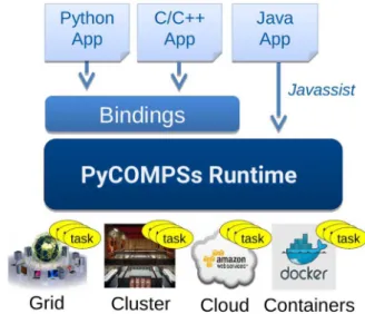
As shown inFigure 1, the PyCOMPSs Runtime allows applications to be executed on top of different infrastruc-tures (such as multi-core machines, grids, clouds or contain-ers) without modifying a single line of the application’s code. Thanks to the different connectors, the Runtime is capable of handling all the underlying infrastructure so that the users only define the tasks. It also provides fault-tolerant mechanisms for partial failures (with job
resubmis-sion and reschedule when task or resources fail), has a live monitoring tool through a built-in web interface, supports instrumentation using the Extrae [19] tool to generate postmortem traces that can be analyzed with Paraver [20,21], has an Eclipse IDE, and has pluggable cloud con-nectors and task schedulers.
Moreover, since the PyCOMPSs Runtime is written in Java [22], Python syntax is supported through a binding, PyCOMPSs. This Python binding is supported by a Binding-commons layer which focuses on enabling the functionalities of the Runtime to other languages (currently, Python and C/C++). It has been designed as an API with a set of defined functions. It is written in C and performs the communication with the Runtime through the JNI [23].
Regarding the programmability,Tasksare identified by the programmer using simple annotations in the form of Python decorators, which indicate that invocations of a given method will become tasks at execution time. The
@taskdecorator also contains information about the direc-tionality of the method parameters specifying if a given parameter is read (IN), written (OUT) or both read and written in the method (INOUT).
Figure 2 shows an example of a task annotation. The parameter cis of type INOUT, and parametersa,b, and
MKLProcare set to the default type IN. The directionality tags are used at execution time to derive the data depen-dencies between tasks and are applied at an object level, taking into account its references to identify when two tasks access the same object. Furthermore, theprioritytag is a hint for the PyCOMPSs’ scheduler that will force to execute the tasks with this tag earlier, always respecting the data dependencies.
Additionally to the @task decorator, the con-straint decorator can be optionally defined to indicate some task hardware or software requirements. Continuing with the previous example, the task constraint Comput-ingUnits shows to the Runtime how many CPUs are consumed by each task execution. The available resources are defined by the system administrator in a separated
XML configuration file. Other constraints that can be defined refer to processor architecture, memory size, etc. Fig. 1. PyCOMPSs overview.
1COMPSs is the task-based programming model for which PyCOMPSs is its Python binding.
A tiny synchronization API completes the PyCOMPSs syntax. As shown in Figure 3, the API function
compss_wait_onwaits until all the tasks modifying the
result’s value are finished and brings the value to the node executing the main program. Once the value is retrieved, the execution of the main program code is resumed. Given that PyCOMPSs is used mostly in distributed environments, syn-chronizing may imply a data transfer from a remote storage or memory space to the node executing the main program.
2.1 PyCOMPSs Runtime
The PyCOMPSs Runtime handles the execution of the applications in the computing infrastructure. The comput-ing infrastructure is composed of several heterogeneous nodes, and the execution is orchestrated following the mas-ter-worker paradigm, where the main program is started on the master node and tasks are offloaded to worker nodes. In the most general case, the node allocating the master node will also allocate a worker node.
As depicted inFigure 4, the Runtime first builds a task graph adding a new node to it every time a task is invoked in the application’s code. The directionality of the parame-ters is used to detect the data dependencies between the new task and previous ones. Secondly, the scheduler will analyze the generated graph in a particular way to execute all the workload among the available resources. We must highlight that this analysis is highly dependent on the differ-ent scheduler implemdiffer-entations, but the Runtime provides information about all the data locations so that they can exploit thedata locality. Eventually, when a task is sched-uled to a given resource, the required objects and files are transferred directly between different memory spaces to guarantee that tasks have available their parameters before execution without passing through the master. Finally, the task is executed in the worker resource and, when specified by the synchronization API, the results are gathered back to the master resource (where the main code is running).
Only concerning the PyCOMPSs binding, when a trans-fer between diftrans-ferent memory spaces is required, the binding serializes and writes the object to disk using the standard library Pickle. The transfer between different resources is then delegated to the Runtime.
Finally, the available Computing Units that each resource can offer to the Runtime is configurable. More specifically, this allows to oversubscribe the amount of work that a resource can receive; meaning that the Runtime can create more threads than the real amount of CPUs that the resource has.
2.2 Interaction with external libraries
The PyCOMPSs Runtime supports the execution of multi-threaded tasks using the constraint interface. The number
of cores assigned to a multi-threaded task can be indicated by the programmer in the ComputingUnits constraint tag. The PyCOMPSs scheduler can assign several cores to a given multi-threaded task. On the other hand, although support for tasks that use several nodes has been added recently, in this work we only consider tasks executing inside a single node.
Before this work, the cores were assigned blindly to the tasks. The performance results observed were relatively poor when running numerical applications, such as those using the NumPy or SciPy libraries that link to the IntelMKL library [24]. It has been shown that, by default, IntelMKL tends to occupy the entire node when the multi-threading is enabled. Not considering this fact can result in a heavy oversubscribing. In addition, each task can be executed in several NUMA sockets. This fact increases the amount of transfers between the different NUMA-nodes, decreasing the performance dramatically. Knowing that this behavior can be found in other libraries, the problem has been solved in a general way.
We have modified the PyCOMPSs task executor in such a way that it is currently able to bind multi-threaded tasks to specific computing units of the infrastructure. This fact, combined with the capability to define the nodes’ virtual amount of computing units, allows the user to achieve the desired rate of oversubscribing. However, this is not done blindly: the PyCOMPSs Runtime distributes the tasks evenly between the different NUMA sockets, avoiding at the maximum the transfers between memory spaces.
2.3 Scheduling infrastructure
PyCOMPSs Runtime has been extended with a scheduling infrastructure that supports pluggable scheduling policies. Almost all the tests presented in this paper are based on
a data locality scheduler that takes into account the node
that stores the data accessed by the tasks. More precisely, a task will have a score equal to the amount of input data present in a given node. It is important to realize that even if a centralized task manager or task scheduler can be a bottleneck in some applications, we are tacking distributed computing platforms and the time required for data trans-fers can be an issue as well, so we are assuming that tasks should have a given granularity that is able to hide the task manager overhead.
Defining a new score policy is enough to change the scheduler behavior. It will prioritize the tasks with the high-est score for a given combination of resource, implementa-tion, and data. In addition to the data locality score, three more policies have been defined: First In First Out (FIFO), Last In First Out (LIFO) and data locality with priority to tasks with a shared edge in the dependency graph with the finished task (FIFOData). In this last policy, there are two different scenarios. In the case where there are tasks freed by the job that has just finished, one Fig. 3. Sample call to synchronization API.
of them is scheduled in First In First Out order; even before treating the tasks that are already free. Otherwise, data
localityis considered between all the available tasks. The
first two policies (LIFO, FIFO) have served to probe the robustness of the scheduling system. The third one can be seen as a relaxation of thedata localityscheduler to lighten the amount of needed comparisons to schedule a task.
The available schedulers allow the users to configure the execution depending on the expected load.
2.4 Python persistent workers
In previous Runtime versions, PyCOMPSs was enhanced with a persistent Java worker, meaning that a Java worker process was started at the beginning of the application execution, communicating with the master to get informa-tion about the tasks to be executed and data transfers to be performed. However, every time a Python task was invoked, a new Python interpreter was launched. This pro-cess has been enhanced with the implementation of Python persistent workers.
More in detail, the PyCOMPSs worker module has been modified on top of the Python’s built-in multiprocessing library. When the application execution begins, the primary worker process in each worker node spawns a set of pro-cesses that will be responsible for executing the tasks. These processes are kept alive during the whole application execu-tion and communicate with the Java persistent worker through pipes. The messages that they exchange include information about the task execution requests, job parame-ters, and computation results. This feature improves the overall performance by reducing the overhead of deploying a new Python interpreter per task. Besides, modules loaded by previous tasks are already present in the interpreter and do not need to be reloaded.
2.5 Methods’polymorphism
GPUs are clearly faster than CPUs for some applications. Nevertheless, it is not always easy to decide whether it is
better to use one architecture or the other [25]. Also, FPGAs are gaining some momentum. In this context, projects with the primary focus of interest on heterogeneous architectures are arising [26]. Hence, it seems reasonable to think that, in both HPC and Big Data contexts, we are going towards environments with heterogeneous architectures.
PyCOMPSs can manage those cases by providing sup-port for the definition of different versions of the same method for different architectures. The programmer can use theimplementsdecorator to indicate that a method implements the same behavior than another.Figure 5shows an example of polymorphism, which together with the
constraintdecorator allows to indicate to the Runtime that some tasks can only be executed in a given set of computing resources. In fact, using polymorphism and tasks’ constraints, the users can define CPU, GPU or FPGA versions of the same task.
Internally, at the beginning of the execution, the Runtime will blindly execute all the available versions that can run in a given resource in order to obtain an execution profile per version. Afterwards, the Runtime is capable to use the profiled information to choose the implementation with the lowest execution time. In this initial version, data size is not taken into account and we take the hypothesis that each kind of implementation is better or worst in the general case. There are no particularities considered capable to combine both implementations depending on the mor-phology of the input data, even if it would be really interest-ing and is can be considered in the future work.
2.6 Profiling
PyCOMPSs generates postmortem traces under demand using Extrae [19]. These files can be explored with Paraver [20, 21], obtaining visual information to make easier the code performance fine tuning.
Some specific PyCOMPSs events have been added in order to differentiate the different steps done by the master Fig. 4. PyCOMPSs Task life-cycle.
and the workers. More precisely, it is possible to see the dif-ferent actions performed by a worker each time that a task is executed.
Finally, the dependency graph generated can be plotted at the end of the computation or be explored on runtime with the monitor.
3 Linear algebra codes
We have evaluated PyCOMPSs with several linear algebra codes. It is important to keep in mind that PyCOMPSs is a general purpose programming model, not a specific one for dense linear algebra computations [27, 28]. Nevertheless, linear algebra algorithms are the base for several fields such as Machine Learning and Computational physics. Even if other good options like ScaLAPACK [29] already do this job, none of them can be called directly from Python. In general, these libraries are coded inCorFortran. They are really low level languages that demand a high encoding effort. In return their can achieve really high performances. On the other hand, PyCOMPSs allows the user to have working versions of an algorithm really quick. In addition, the dynamic runtime scheduling empowers the resource efficiency increasing the performance. It is so perfect for prototyping and verifying new concepts and ideas and, as will be shown, can even be competitive under the efficiency point of view.
In general, the matrices are chunked in smaller square matrices (blocks) to distribute the data easily along the available resources and take advantage of this fact to con-sider the square blocks as the minimum entity to work with [30]. All the operations performed on the blocks use the best library available for each architecture, either IntelMKL or
PyCUDA[31] throughskcuda[32].
The following schema has been pursued for all the com-putations. The initialization is performed in a distributed way, defining tasks to initialize the matrix blocks. These tasks do not take into account the nature of the algorithm and they are scheduled in a round robin manner. Next, all the computations are done considering that the data is already allocated in a given node. The data locality sched-uler will assign the tasks taking into account the locality information and reducing the data transfers. This method-ology shows that PyCOMPSs is capable of obtaining HPC
performance in Big Data environments, where data is already present in the infrastructure, and it is not possible to arrange its location depending on the computation.
The following subsections provide a brief description of the encoded algorithms.
3.1 Matrix multiplication
The matrix multiplication code performs a matrix multipli-cation by blocks. The code has two tasks: one for the creation of the matrices’ blocks and one for the blocks’ multiply-accumulate. Since the blocks are defined as NumPy arrays, the operations that operate on them are overridden and the corresponding NumPy operation is invoked, which calls as well to the IntelMKL operation. Notice that this behavior happens even when indicated with arithmetic operators.
Figure 2shows the code used to perform the multiplica-tion task. The computamultiplica-tional complexity of this algorithm is widely known: 2S3, whereSis the side size of the matrix. In this context, it may be easier to noteS=N·Mwhere Nis the amount of blocks in a side andMis the side size of a single block.
3.2 Cholesky factorization
The Cholesky factorization can be applied to Hermitian positive-defined matrices. This decomposition is a particu-lar case of the LU factorization, obtaining two matrices of the formU = Lt.
There are two main blocked algorithms to perform a Cholesky decomposition. The right-looking algorithm [33] and the left-looking version [34].Figure 6 shows the code used in this case, corresponding to the right-looking approach. It has been chosen because it is more aggressive, meaning that in an early stage of the computation there are blocks of the solution that are already computed and all the potential parallelism is released as soon as possible. Hence, the Runtime can continue performing the following compu-tations on the matrices.
The functions in bold in the Cholesky code (potrf,
solve_triangular, andgemm) are annotated as tasks. Each of these tasks internally calls to IntelMKL functions, with a given number of threads.
Figure 7 shows the code of the potrf task from the Cholesky code. This task has a constraint decorator Fig. 6. Cholesky factorization main function.
that indicates the number ofComputingUnits(CPU’s in this case) required to execute the task that, during the experimentation, matches the amount of IntelMKL threads. Notice that the PyCOMPSs Runtime can be configured to oversubscribe the computing nodes with tasks that involve more threads than the actual available computing cores. This way we can overlap I/O operations when starting/ending tasks with the actual computation, increasing the resource efficiency. The other tasks defined in this example look very similar to thepotrfone.
On the other hand, this kernel has a GPU version. The PyCOMPSs Runtime automatically handles the GPUs present in a node setting wisely the CUDA visible devices. Figure 8shows how easy is to take advantage of the accel-erators. The polymorphism syntax explained inSection 2is used to give an alternative version ofdgemm. The user can consider the presented code as a template and just change the call tocuBLASwith the desired kernel. Hence, even if the code can seem a little bit complicated, it allows a user that has never seen a line ofCUDAto use the GPUs from Python in a distributed context.
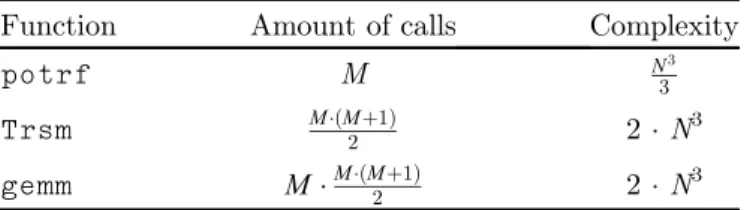
Looking at the code and considering the complexity of each call, it is possible to build the Table 1. Hence, the complexity of the algorithm can be computed as shown in Figure 9, where M is the amounts of blocks per side and Nthe side block size. We can conclude that the algorithm is OðMN3Þ3that is the same complexity of the sequential algorithm.
3.3 QR factorization
Traditional QR algorithms use the Householder trans-formation, but this method requires accessing a whole column of the matrix, while our data structures are based on blocks. The approach followed in our implementa-tion uses a method based on Givens rotaimplementa-tions, which access the data in the matrices by blocks [35]. While the Cholesky approach is the well known typical one, in the QR we have to follow a more complicated procedure to achieve a good degree of parallelism. The following steps are followed:
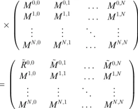
1. Decomposition of the input matrix in blocks
A¼ M0;0 M0;1 . . . M0;N M1;0 M1;1 . . . M1;N .. . MN;0 .. . MN;1 . . . . . . .. . MN;N 0 B B B B @ 1 C C C C A
2. QR decomposition of the upper left block
Mi;j¼Qi;iR~ii;i!A0 ¼ ðQ0;0Þt 0 . . . 0 0 I . . . 0 .. . 0 .. . 0 . . . . . . .. . I 0 B B B B B @ 1 C C C C C A Fig. 8. dgemmtask executed in the GPU.
Table 1. NumPy calls done to perform a Cholesky decomposition.
Function Amount of calls Complexity
potrf M N33
Trsm MðM2þ1Þ 2N3
gemm MMðM2þ1Þ 2N3
Fig. 9. Cholesky complexity. Fig. 7. potrf task in the Cholesky code.
M0;0 M0;1 . . . M0;N M1;0 M1;1 . . . M1;N .. . MN;0 .. . MN;1 . . . . . . .. . MN;N 0 B B B @ 1 C C C A ¼ ~ R0;0 M~0;1 . . . M~0;N M1;0 M1;1 . . . M1;N .. . MN;0 .. . MN;1 . . . . . . .. . MN;N 0 B B B @ 1 C C C A 3. Change every block of the column for zero blocks a. Rotation matrix construction through a partial QR decomposition ~ Rij;i ~ Mjþ1;i ! ¼ R 0;0 C0;1 C1;0 R1;1 ! ~ Rij;þi1 0 ! ! R~ i;i jþ1 0 ! ¼ R 0;0 t C1;0 t C0;1 t R1;1 t ! ~ Rij;i ~ Mjþ1;i
b. Add the rotation matrix to introduce a new zero block in theRmatrix
A00 ¼ R0;0 t C1;0 t . . . 0 C0;1 t R1;1 t . . . 0 .. . 0 .. . 0 . . . . . . .. . I 0 B B B B B @ 1 C C C C C A Q0;0 t 0 . . . 0 0 I . . . 0 .. . 0 .. . 0 . . . . . . .. . I 0 B B B @ 1 C C C A M0;0 M0;1 . . . M0;N M1;0 M1;1 . . . M1;N .. . MN;0 .. . MN;1 . . . . . . .. . MN;N 0 B B B @ 1 C C C A ¼ ~ R01;0 M~0;1 . . . M~0;N 0 M~1;1 . . . M~1;N .. . MN;0 .. . MN;1 . . . . . . .. . MN;N 0 B B B @ 1 C C C A
c. Repeat the previous procedure with all the elements in the column, obtaining the following expression
ANÞ ¼Q~0A¼ ~ RN0;0 M~N0;1 . . . M~0N;N 0 M~1;1 . . . M~1;N .. . .. . . . . .. . 0 MN;1 . . . MN;N 0 B B B B B B B @ 1 C C C C C C C A ¼ R 0;0 ½M0 A0
4. Return to the point 1, treating the submatrix result of discarding the first row and the first column of the obtained AN)Once all the transformations have been performed, the following expression is obtained:
R¼Q~NQ~N1. . . ~Q1Q~0A 5. Compute the final Q
^
Q¼Q~NQ~N1. . . ~Q1Q~0!R¼QA^ !A¼Q^tR!Q¼Q^t Figure 10 shows the QR implementation used in this paper that corresponds to the previous algorithm. An aux-iliary matrix, mainly composed of identity and zero blocks except for the four blocks corresponding to the posi-tions (i,i), (i,j), (j,i)and (j,j), where (i,j) is the position that is being rotated (changed to zero) performs the rota-tions. Although in our initial version of the QR algorithm we were allocating this auxiliary matrix, we have developed a second version where only those blocks different to iden-tity or zero are actually allocated, and only the multiplica-tions by values different to identity or zero are performed. With this second approach (calledmemorySaveQRin the evaluation), we save memory space and reduce useless computations.
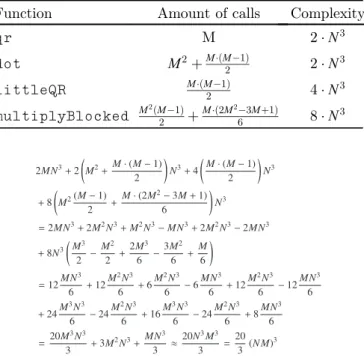
Once again, the complexity can be deduced from the code considering the complexity of each call, building the Table 2. Thus, as demonstrated inFigure 11, the complex-ity of the algorithm is O (20 (NM)3). In this case, the obtained complexity is larger than the sequential one even if it is in the same order. Nevertheless, the parallelism obtained is remarkable so if the main goal is to make the algorithm scalable, the trade-off is worth.
3.4 LU factorization
In this case, an approach without pivoting [36] has been the starting point. The partial pivoting blocked algorithm [37] was not considered because requires an entire column to be present in a node to compute the partial column LU decom-position. Knowing that this approach is unstable in general [38], one modification has been done to increase the stability of the algorithm while keeping the block division and avoid-ing bravoid-ingavoid-ing an entire column into a savoid-ingle node.
Figure 12shows a schema with all the steps taken in an iteration of the LU factorization:
1. The current principal block, considered the one with the lowest column and row index (A in the figure) is decomposed using some underlying library.
2. The firstU’s row (U12in the figure) is computed using the row of the current principal block.
3. The column of the present main block is used to calcu-late an auxiliary result for the next steps (P22L21). 4. The LU decomposition of the blocks with a row or
column index larger than the principal one is launched (recursive step).
5. The first L’s column (L21 in the figure) is computed using the column of the current main block as well as the result of the iterative step.
Finally,Figure 13shows the code corresponding to the previously presented algorithm.
In the previous cases, all the calls had a cubic complex-ity. On the other hand, this kernel has some calls like
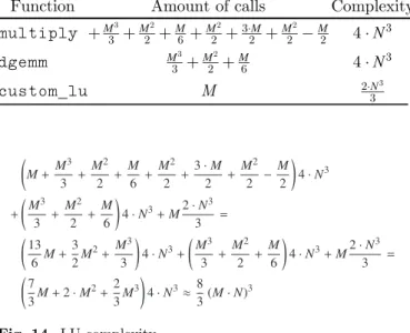
invert_triangular – which calls to solve_trian-gular, the MKL function to invert triangular matrices – with quadratic complexity that have been neglected, build-ingTable 3. InFigure 14all the terms have been added to compute the total complexity which is ¼ 8
3ðM NÞ 3
. Since in sequential a developer would use either a non pivoting algorithm or a pivoting considering the full columns, it makes no sense to compare the complexity of this algorithm against the sequential code. Nevertheless, it is interesting to realize that it is less than a half of the QR asymptotic complexity.
Table 2.NumPy calls to perform a QR decomposition.
Function Amount of calls Complexity
qr M 2N3
dot M2þMðM21Þ 2N3
littleQR MðM21Þ 4N3
multiplyBlocked M2ðM21ÞþMð2M263Mþ1Þ 8N3
Fig. 11. QR complexity.
Fig. 12. LU mathematical principles.
Fig. 13. LU factorization main function. Fig. 10. QR factorization main function.
4 Results
4.1 Computing infrastructure
The execution results presented in this section have been obtained in three different clusters located at theBarcelona
Supercomputing Center(BSC).
We have used PyCOMPSs version 2.2 for the initial evaluations, and the same version with the Python persis-tent workers to test these new features. We have also used IntelPython 2.7.13 and IntelMKL 2017.
MareNostrum III
This supercomputer was composed by 3056 nodes, each of them with two Intel SandyBridge-EP E5-2670/1600 20M (8 cores at 2, 6 GHz each), main memory that varies from 32 to 128 GB, FDR-10 Infiniband and Gigabit Ethernet network interconnections, and 3 PB of disk stor-age [39]. It was providing service for researchers from a wide range of different areas, such as life science, earth science and engineering until March 2017.
COBI cluster
This cluster is an IntelSSF system composed of 8 nodes with two Intel Xeon CPU E5-2690 v4 @ 2.60 GHz and 128 GB of main memory each (Xeon nodes) and 8 nodes with an IntelXeon PhiCPU 7210 @ 1.30 GHz and 110 GB of main memory each (KNL nodes). The network technology used is Omni-Path. Also, Lustre [40] is used as shared file system.
Minotauro cluster
This cluster is composed of 61 nodes with two IntelE5649 @ 2.53 GHz, 2 M2090 NVIDIA GPU cards and 24 GB of main memory each with two Infiniband QDR ports and 39 nodes with two IntelE5-2630 v3 @ 2.4 GHz, 2 K80
NVIDIA GPU cards (2 NVIDIA Kepler GK210 each) and 128 GB of main memory with 1 PCIe 3.0 Mellanox ConnectX-3FDR 56 Gbit port.
4.2 General comments on the evaluation
We consider that Python users will use the intra-node parallelized version of the linear algebra algorithms through MKL (not only a shared memory implementation, but a one optimized for Intel processors) into their applications. Since these kernels can be directly called from Python with-out any further installation, we have considered them as a really good reference point for Cholesky, QR, and LU. Hence, instead of comparing thePyCOMPSs implementa-tions against other distributed kernels, we have computed
the SpeedUp’s against the sequential version encoded to
be optimal for this kind of processor. Since the sequential version has shared memory and does not perform transfers, we consider that having a good performance when compar-ing against these executions is enough to assess the good behavior of the executions.
On the other hand, it is important to keep in mind that, for a given matrix size, increasing the block size implies decreasing the number of total blocks. Hence, even if we show that better performances can be obtained when increasing the block size, this fact decreases the number of blocks and thus the maximum parallelism. Moreover, since the input sizes are bigger, each task requires a higher amount of memory. After considering all these factors and trade-offs, we have decided to perform all the tests with blocks of 4K·4K.
Finally, we would like to highlight the fact that, for most of the executions, we delegate the transfers to the shared file system. Hence, it is difficult to evaluate accu-rately the transfer time since the shared file systems have lots of data cached in memory and replicated across the cluster. This is the main reason why this study has not been done.
4.3 Matrix multiplication
For the matrix multiplication example, we have first analyzed the impact of the oversubscription in a single node of MareNostrum III. The data square matrices considered had 32K·32K doubles, organized in blocks of 4K and 8K. Larger blocks have not been tested since there is a limit on the serialization size for a single block of 4 GB for Python 2.7. This limitation is due to a hardcoded parame-ter in thesave_bytesfunction, present in the class_pickle.c of the module in charge of the serializations.
We have instructed the Runtime to schedule always two tasks per NUMA socket, where all task threads are bounded to a single socket as described inSection 2. The number of threads in each execution ranged from 4 to 32 threads, in such a way that the oversubscription ratio ranged from 1 (when 4 threads/task are used) to 8 (when 32 threads/task are used). Figure 15shows the results of this evaluation. Notice that PyCOMPSs gets the maximum performance when using a level of oversubscription of 4 and a block size of 8K. The performance in the best case is around Table 3.NumPy calls to perform a LU decomposition
Function Amount of calls Complexity
multiply þM3 3 þ M2 2 þ M 6 þ M2 2 þ 3M 2 þ M2 2 M 2 4N 3 dgemm M33þM2 2 þ M 6 4N 3 custom_lu M 2N3 3 Fig. 14. LU complexity.
200 GFLOPS, which represents the 60% of the peak of a MareNostrum III node (332 GFLOPS [41]).
Next, we have executed the same PyCOMPSs code in a variable number of nodes of MareNostrum III, from 1 to 64 (from 16 to 1024 cores), with an additional node for the master.
Figure 16shows the performance obtained with matri-ces of 64K·64K doubles, organized in blocks of 4K·4K. The Runtime was configured to execute a maximum of four tasks per node, each of them using 16 IntelMKL threads, which represent an oversubscription ratio of four. The light green line labeledIdeal distributed scalingis derived by con-sidering an ideal speedup from the performance obtained in one node with PyCOMPSs. The red lineSequential
perfor-mance corresponds to the performance obtained with
IntelMKL in one node with 16 threads for a single block of 4K·4K (251 GFLOPS). We observe a very good speedup until 16 nodes. After that, the efficiency is lower but the system keeps scaling.
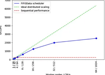
The next result worth mentioning concerning the matrix multiplication is the heterogeneous execution in the COBI cluster.Figure 17shows a post-mortem trace file obtained with Extrae and analyzed with Paraver. More pre-cisely, the execution uses one Xeon node and one KNL node. Blue tasks at the left-side of the image correspond to initialization tasks and the white ones to block multipli-cations. Green flags point out beginning and end of tasks. Notice that these many-core architectures allow working with plenty of tasks simultaneously. For instance, this exe-cution multiplies two matrices of 131K·131K divided into blocks of 4K, with 1024 free tasks in average, and a total amount of 32 768 tasks; showing the capability of the PyCOMPSs Runtime to handle a huge amount of work. Each KNL node executes four tasks concurrently and each Xeon node executes eight tasks at a time.
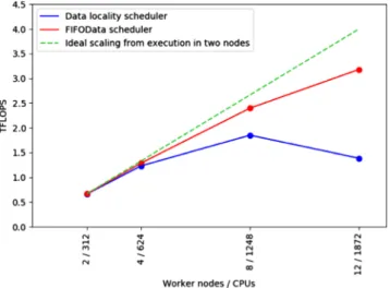
In this context, and considering that there is not a ded-icated node to allocate the master (it runs in a Xeon node that also executes an entire worker), the scalability study has stressed the scheduler.Figure 18shows how the Data locality scheduler degrades much faster than the FIFOData
scheduler. This is due to the simplification in the second scheduling policy, avoiding a lot of comparisons between the score of the different free tasks. In this case, the users have two options to increase the performance, either to change the scheduler or to dedicate more resources to the Runtime.
We have so demonstrated the importance of the choice both of the block size and the scheduler choice. In addition, we show that a good performance on the matrix multiplica-tion can be achieved until 16–32 nodes. Finally, we show that PyCOMPSs Runtime is able to handle different imple-mentations of the same function to take advantage of heterogeneous infrastructures.
Fig. 15. Matrix multiplication evaluation inside one node: impact of oversubscription.
Fig. 16. Matrix multiplication performance in a distributed cluster.
Fig. 17. Matrix multiplication heterogeneous execution trace in the COBI cluster.
4.4 Cholesky factorization
Figure 19 shows the Cholesky performance in MareNos-trum III. The matrix size is again 64K·64K doubles, and the block size is 4K·4K doubles. We have used the same values for the maximum tasks per node and oversub-scription than in the previous case (4 tasks per node, 16 threads per task, and an oversubscription ratio of 4).
The red lineSequential performancecorresponds to the performance obtained with IntelMKL potrf with 16 threads for a block of 4K·4K doubles (72 GFLOPS) in a single MareNostrum node. The green lineIdeal scaling
from sequentialis equivalent to the ideal speedup calculated
from the previous value.
The chart shows the performance result with PyCOMPSs 2.2. The line shows ideal scaling up to four nodes and an increasing degradation from there.
When inspecting the post-mortem performance traces, we have observed that the degradation of the performance is due to the morphology of the task-graph. Combining the observed results shown inFigures 20and21, the maximum available parallelism is already filled with eight nodes. We can conclude this by looking at the inverse triangle form of the DAG and the resource fulfillment of the resources in the trace. This is a good example of how useful the pro-filing tools can be when analyzing the code to understand the obtained performance.
Figure 22 shows the performance obtained with a heterogeneous execution in the COBI cluster. The block size is 4K·4K and the matrix size is 130K·130K. For each execution, half of the nodes are Xeon, and half are KNL nodes. In this case, only thegemmfunction can run on both architectures. The rest can run only in the Xeon nodes.
Figure 20shows the execution trace of the previous per-formance test with four Xeon and four KNL nodes. Green segments correspond to initialization tasks, the blue ones topotrf, the red ones to solve_triangularand the white ones to gemm. Yellow lines separate the different nodes. While the nodes with a maximum of four tasks run-ning at a time are KNLs, the ones with a maximum of eight
are Xeon nodes. In this execution, the KNL nodes are con-strained to executegemmtasks and readers may notice that the scheduler is capable of handling the fact that not all the machines can execute all tasks’ types by only sending the tasks where they can run.
Finally, two executions in the Minotauro cluster have been performed. This is an heterogeneous cluster with two different types of node. It this case, no performance studies have been done. This is mainly due to the fact that considering that each time a GPUs is used, the data has to be copied to its memory and bring back the result. This slows down the execution significantly compared to the maximum theoretical performance. Nevertheless, it is important to realize that the PyCOMPSs Runtime is able to handle a double heterogeneity in this case. On a first level, we have two different kind of nodes in the cluster. On a second level, each one of those nodes has two different kind Fig. 19. Cholesky performance in MareNostrum III.
Fig. 20. Cholesky decomposition heterogeneous execution trace in the COBI cluster.
Fig. 18. Performance of a 131K·131K double matrix multi-plication heterogeneous execution in the COBI cluster.
of processors: several CPUs and GPUs. PyCOMPSs Run-time handles successfully four different types of processors in a single execution with a minimum effort for the devel-oper.Figure 23shows the traces obtained when using two (Fig. 23a) and four nodes (Fig. 23b). In each case, half the nodes are of one type and half of the other. The main interest of these executions is to show that we are able to execute a kernel in an heterogeneous GPU cluster. Still, the perfor-mance remains really poor since all the data is copied between the CPU and the GPU memory each time a compu-tation is done. We think that the performance could be increased implementing a cache to handle the GPU mem-ory, avoiding some data transfers. Nevertheless, this remains as an idea for future work.
4.5 QR factorization
For the QR evaluation, we used a matrix of size 32K·32K doubles organized in blocks of 4K·4K doubles. We have evaluated the dense version of the factorization against the memory save version. As described inSection 3.3, the Fig. 23. Cholesky factorization: heterogeneous execution trace
of a 16 blocks·16 blocks matrix.
Fig. 21. Cholesky dependency graph for a 16 blocks·16 blocks matrix decomposition.
difference between both versions is that the sparse version only allocates those blocks of the auxiliary matrix that are different to the identity or to zero. Additionally, the operations with this identity or zero blocks are not performed (the original block or a zero block is directly returned). To accomplish this behavior, each element is modeled as a list with an integer to indicate the block type and, if necessary, a NumPy array with its real content.
Figure 24 presents the results obtained executing the code in MareNostrum III. As explained in the previous case, the application does not scale well beyond 4 nodes because it reaches the parallelism limit of the application. Neverthe-less, the performance until this point is excellent.
Figure 25shows the dependency graph corresponding to a QR decomposition of a 4 blocks·4 blocks execution, manifesting that the PyCOMPSs Runtime is not only able to handle an enormous amount of tasks but also really com-plex dependency graphs. The real execution (8 blocks·8 blocks) has a much more complicated graph but is too large to be depicted in this paper.
4.6 LU factorization
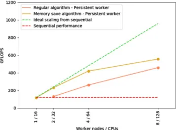
In this case, all the executions have been performed in the COBI cluster using only Xeon nodes. A matrix with 82K·82K doubles has been factorized, obtaining the matricesP,L andUdetailed inSection 3.4.
As shown in Figure 26, the reference execution perfor-mance is the maximum achieved with a threaded code executing pure NumPy code, corresponding to a 32K·32K doubles matrix. The performance obtained with a matrix with 4K·4K doubles (the block size used in the dis-tributed execution) is 41 GFLOPS, far away from the 218 GFLOPS achieved with the 32K·32K matrix. This fact suggests that when the matrix is not large enough, not all the resources are fulfilled. Nonetheless, when execut-ing several tasks at the same time, PyCOMPSs takes advantage of all the available resources.
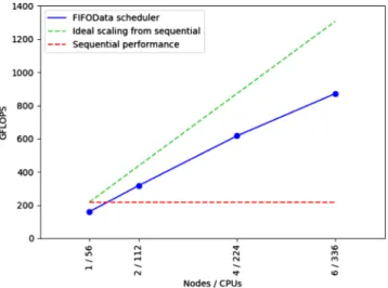
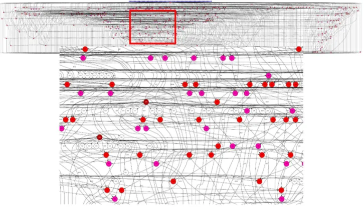
Two remarkable facts can be deduced from this experi-ment. The blocked LU decomposition scales pretty well until a reasonable amount of cores. In addition, the PyCOMPSs Runtime demonstrates its capacity to work with really complicated DAGs.Figure 27shows a zoom of a dependency graph for a 8 blocks·8 blocks execution that makes easier to appreciate the complexity handled by the PyCOMPSs Runtime. On the other hand,Figure 28shows the dependency graph for a 6 blocks·6 blocks execution.
On the other hand, not only the DAG complexity is important. The amount of tasks that the Runtime can handle is also remarkable. In this case, we have observed that the scheduler choice has a really big impact in the final performance.Figure 29ashows that, in this case, the data locality scheduler is not the best choice. It adds come over-head to compute the best locality when, in fact, all the data is directly available on lustre. When taking into account this fact, the FIFOData scheduler has been considered. Figure 29b shows that the obtained performance is much better. In this execution, 34 288 tasks are executed in 380 seconds in 196 cores. Figure 29c shows that with this amount of tasks and slots available, the Runtime is able to run correctly with tasks that last 0.7–2.0 s. Hence, the throughput is in the microseconds order. This execution can serve as example to better understand PyCOMPSs Fig. 25. QR dependency graph for a 4 blocks·4 blocks matrix decomposition.
Fig. 26. LU performance in the COBI cluster with Xeon nodes.
capabilities since is handles a huge amount of tasks not last-ing so much.
4.7 Programming complexity
As stated inSection 2, we aim at providing a programming model that makes it easier the development of parallel applications. While it is difficult to evaluate the easiness or complexity of a programming model, we show in this subsection a summary of the lines of code required to pro-gram the PyCOMPSs codes described in this paper as a measure for programmability.
These codes are composed of the main algorithm and the tasks’ functions. The main algorithm is usually expressed in a method, like the ones shown in Figures 6,
10or 13, with lengths of 15–30 lines composed of a set of nested loops with calls to the task functions. The task func-tions are much simpler, each of them of 5–10 lines (like the ones inFigures 2or7) and are wrappers to the NumPy calls with the corresponding PyCOMPSs decorators.
Table 4shows a summary of the lines required to program all the codes presented in this paper. The Main function col-umn is the number of lines in the main algorithm of the codes. The Program column is the total number of lines. The col-umn Decorator corresponds to the number of lines specific for PyCOMPSs, that can be considered the added lines to a sequential version of the code. We can see that from very simple codes, we can obtain performance in distributed and heterogeneous platforms. Readers must consider that the codes contain spaces and blank lines to ease its Fig. 27. LU dependency graph for a 8 blocks·8 blocks matrix.
comprehension and that they include the distributed matrix initialization, the auxiliary functions to join the blocked matrix for the result verification, and the timers to com-pute the elapsed time. Hence, the number of lines can be
considered a superior bound (which could be easily reduced) of a complete program that tests the correct behavior of the kernels. Furthermore, we explicitly state the number of lines added as decorators to obtain the distributed version from the blocked one. We highlight that it makes no sense to com-pare the distributed version against the sequential one since all the kernels can be called in a single MKL line.
5 Conclusion
PyCOMPSs is a robust programming model that enables the programmer to achieve remarkable performances with clean and simple codes. Based on the sequential version and just by adding some decorators skillfully, the code is ready to run on distributed and heterogeneous clusters thanks to the power of the Runtime that automatically handles all the tasks’ scheduling and data transfers. Once the Runtime is installed on a given infrastructure, the code parallelized with PyCOMPSs is easily executed.
This paper has shown that good performances can be achieved regarding sequential codes when calling lower level libraries tuned for each particular architecture. PyCOMPSs allows the users to quickly turn a Python sequential code into a highly portable distributed version. Depending on the code’s nature, PyCOMPSs can so play both the distributed programming language and orchestrator roles. In fact, when increasing the size of the matrices, we are able to take advan-tage of all the architecture, observing super linearSpeedUp’s when considering the sequential execution as the reference.
Finally, all the executions have been performed with the data already present in the shared file system. The PyCOMPSs Runtime has shown that it is capable of achieving a good performance level when the data is already present in the infrastructure. This fact puts the program-ming model in the frontier between Big Data and HPC, ful-filling the needs of both environments.
Acknowledgments. This work has been supported by the Spanish Government (SEV2015-0493), by the Spanish Ministry of Science and Innovation (contract TIN2015-65316-P), by Generalitat de Catalunya (contracts 2014-SGR-1051 and 2014-SGR-1272). Javier Conejero postdoctoral contract is co-financed by the Ministry of Economy and Competitiveness under Juan de la Cierva Formacio´n postdoctoral fellowship number FJCI-2015-24651. Cristian Ramon-Cortes predoctoral contract is financed by the Ministry of Economy and Competi-tiveness under the contract BES-2016-076791. This work is supported by the Intel-BSC Exascale Lab.
This work has been supported by the European Commission through the Horizon 2020 Research and Innovation program under contract 687584 (TANGO project).
References
1 Stephen Cass (2017)The 2017 Top Programming Languages (IEEE Spectrum), https://spectrum.ieee.org/comput-ing/software/the-2017-top-programming-languages,
accessed: 2018-02-14. Fig. 29. LU decomposition execution trace of a 32 blocks·32
blocks matrix with 2048·2048 blocks.
Table 4.Amount of code lines in each kernel.
Algorithm Main function Program Decorator matmul MN31 7 66 4 matmul COBI2 7 91 7 cholesky MN31 22 136 8 cholesky COBI2 22 147 11 cholesky Minotauro3 22 170 11 QR MN31 31 233 10 memorySaveQR MN31 31 310 14 LU COBI1 45 155 10 1 Homogeneous. 2
dgemm versioning Xeon-KNL. 3
4 Jones E, Oliphant E., Peterson P. (2001)SciPy: Open source scientific tools for Python,http://www.scipy.org/
5 BLAS (Basic Linear Algebra Subprograms)Web page at http://www.netlib.org/blas/, accessed: 28th August, 2017. 6 Anderson E., Bai Z.J., Bischof C., Susan Blackford L.,
Demmel J., Dongarra J., Du Croz J., Greenbaum A., Hammarling S., McKenney A.,et al.(1999) LAPACK Users’
guide,SIAM.
7 Dagum L., Menon R. (1998) OpenMP: An Industry-Standard API for Shared-Memory Programming,IEEE Comput. Sci. Eng.5,1, 46–55,https://doi.org/10.1109/99.660313. 8 Threading Building Blocks (IntelTBB) (2017) Web page at
https://www.threadingbuildingblocks.org/, accessed: 28th August, 2017.
9 Parallel Processing and Multiprocessing in Python (2017) Web page at https://wiki.python.org/moin/ParallelProcess-ing, accessed: 10th October, 2017.
10 Parallel Python Software (2017) Web page at http:// www.parallelpython.com, accessed: 10th October, 2017. 11 Dalcı´n L., Paz R., Storti M. (2005) MPI for Python, J.
Parallel. Distr. Com.,http://www.sciencedirect.com/science/ article/pii/S0743731505000560.
12 Tejedor E., Becerra Y., Alomar G., Queralt A., Badia R.M., Torres J., Cortes T., Labarta J. (2017) PyCOMPSs: Parallel computational workflows in Python,Int. J. High Perform. Comput. Appl.31,1, 66–82.
13 Ramon-Cortes C., Serven A., Ejarque J., Lezzi D., Badia R.M. (2018) Transparent orchestration of task based parallel applications in containers platforms,J. Grid Computing16,
1, 137–160.
14 Dask Development Team (2016)Dask: Library for dynamic task scheduling,http://dask.pydata.org
15 PySpark (The Spark Python API (2017) Web page at https://spark.apache.org/docs/latest/api/python/in-dex.html, accessed: 6th October, 2017.
16 McKinney W. (2011) pandas: a foundational python library for data analysis and statistics,Python for High Performance and Scientific Computing1–9.
17 Zaharia M., Chowdhury M., Franklin M.J., Shenker S., Stoica I. (2010) Spark: Cluster Computing with Working Sets, in:Proceedings of the 2Nd USENIX Conference on Hot Topics in Cloud Computing, Berkeley, CA, USA.
18 Conejero J., Corella S., Badia Rosa M., Labarta J. (2017) Taskbased programming in COMPSs to converge from HPC to big data, Int. J. High Perform. Comput. Appl. 4, https://doi.org/10.1177/1094342017701278.
19 Extrae Web page at https://tools.bsc.es/extrae, accessed: 19th December, 2016.
20 Pillet V., et al. (1995) Paraver: A tool to visualize and analyze parallel code,Transputer and Occam Developments 4,17–32,http://www.bsc.es/paraver.
21 Paraver: a flexible performance analysis tool Web page at https://tools.bsc.es/paraver, accessed: 19th December, 2016.
22 Lordan F., Tejedor E., Ejarque J., Rafanell R., A´ lvarez J., Marozzo F., Lezzi D., Sirvent R., Talia D., Badia R.M. (2014) ServiceSs: An Interoperable Programming Framework for the
ence Manual, Intel Corporation, Santa Clara, USA, ISBN 630813-054US.
25 Che S., Boyer M., Boyer M., Meng J., Tarjan D., Sheaffer J.W., Lee S.-H., Skadron K. (2009) Rodinia: A benchmark suite for heterogeneous computing, in:Proceedings of the 2009 IEEE International Symposium on Workload Charac-terization (IISWC), IISWC ’09 IEEE Computer Society, pp. 44–54,http://dx.doi.org/10.1109/IISWC.2009.5306797. 26 Djemame K., Armstrong D., Kavanagh R.E., Deprez J.-C.,
Ferrer A.J., Garcı´a-Pe´rez D., Badia R.M., Sirvent R., Ejarque J., Georgiou Y. (2016) TANGO: Transparent heterogeneous hardware Architecture deployment for eNergy Gain in Operation,http://arxiv.org/abs/1603.01407. 27 Chan E., Van Zee F.G., Bientinesi P., Quintana-Orti E.S.,
Quintana-Orti G., van de Geijn R. (2008) SuperMatrix: a multithreaded runtime scheduling system for algorithms-by-blocks, in:Proceedings of the 13th ACM SIGPLAN Sympo-sium on Principles and practice of parallel programming, PPoPP’08, ACM, pp. 123–132,http://doi.acm.org/10.1145/ 1345206.1345227.
28 Agullo E., Demmel J., Dongarra J., Hadri B., Kurzak J., Langou J., Ltaief H., Luszczek P., Tomov S. (2009) Numer-ical linear algebra on emerging architectures: The PLASMA and MAGMA projects,J. Phys. Conf. Ser.180,1, 012–037, http://stacks.iop.org/1742-6596/180/i=1/a=012037. 29 Blackford L.S., Choi J., Cleary A., D’Azevedo E., Demmel J.,
Dhillon I., Dongarra J., Hammarling S., Henry G., Petitet A., Stanley K., Walker D., Whaley R.C. (1997) ScaLAPACK Users’Guide,Society for Industrial and, Applied Mathematics.
30 Gunnels J.A., Gustavson F.G., Henry G.M., van de Geijn R.A. (2001) FLAME: Formal Linear Algebra Methods Environment, ACM Trans. Math. Softw. 27, 4, 422–455, http://doi.acm.org/10.1145/504210.504213.
31 Klo¨ckner A., Pinto N., Lee Y., Catanzaro B., Ivanov P., Fasih A. (2012) PyCUDA and PyOpenCL: A scripting-based approach to GPU run-time code generation, Parallel Com-puting 38, 3, 157–174, ISSN 0167-8191. https://doi.org/ 10.1016/j.parco.2011.09.001.
32 Givon L.E., Unterthiner T., Benjamin Erichson N., Wei Chiang D., Larson E., Pfister L., Dieleman S., Lee G.R., van der Walt S., Menn B., Mihai Moldovan T., Bastien F., Shi X., Schlu¨ter J., Thomas B., Capdevila C., Rubinsteyn A., Forbes M.M., Frelinger J., Klein T., Merry B., Merill N., Pastewka L., Clarkson S., Rader M., Taylor S., Bergeron A., Ukani N.H., Wang F., Zhou Y. (2015) scikit-cuda 0.5.1: a Python interface to GPU-powered libraries, http://dx.doi.org/ 10.5281/zenodo.40565.
33 Bientinesi P., Gunter B., van de Geijn R.A. (2008) Families of Algorithms Related to the Inversion of a Symmetric Positive Definite Matrix,ACM Trans. Math. Softw.35,1, 1– 3,http://doi.acm.org/10.1145/1377603.1377606.
34 Ltaief H., Tomov S., Nath R., Du P., Dongarra J. (2011) A scalable high performant Cholesky factorization for multicore with GPU accelerators, in: Proceedings of the 9th Interna-tional Conference on High Performance Computing for Computational Science, VECPAR’10, Springer-Verlag, pp. 93–101,http://dl.acm.org/citation.cfm?id=1964238.1964251
35 Quintana-Orti G., Quintana-Orti E.S., Chan E., van de Geijn R.A., Van Zee F.G. (2008) Scheduling of QR Factorization Algorithms on SMP and Multi-Core Architectures, in: Proceedings of the 16th Euromicro Conference on Parallel, Distributed and Network-Based Processing (PDP 2008), PDP ’08, IEEE Computer Society, pp. 301–310, http:// dx.doi.org/10.1109/PDP.2008.37..
36 Golub Gene H., Van Loan C.F. (1996)Matrix Computations, 3rd edn., Johns Hopkins University Press, Baltimore, MD, USA, ISBN 0-8018-5414-8.
37 Quintana-Ortı´ E.S., van de Geijn R.A. (2008) Updating an LU factorization with pivoting, ACM Trans. Math. Softw. 35, 2, 1–11, http://doi.acm.org/10.1145/1377612. 1377615.
38 Demmel James W., Higham Nicholas J. (1992) Stability of Block Algorithms with Fast Level-3 BLAS, ACM Trans. Math. Softw. 18, 3, 274–291, http://doi.acm.org/10.1145/ 131766.131769.
39 MareNostrum III User’s GuideWeb page at https:// www.bsc.es/support/MareNostrum3-ug.pdf, accessed: 21st August, 2017.
40 Architecting a High Performance Storage SystemWeb page at https://www.intel.com/content/dam/www/public/us/ en/documents/white-papers/architecting-lustre-storage-white-paper.pdf, accessed: 21st August, 2017.
41 Intel Xeon Processor E5-2600 SeriesWeb page at http://download.intel.com/support/processors/xeon/sb/ xeon_E5-2600.pdf, accessed: 21st August, 2017.