Aas, Czado, Frigessi, Bakken:
Pair-copula constructions of multiple dependence
Sonderforschungsbereich 386, Paper 487 (2006)
Online unter: http://epub.ub.uni-muenchen.de/
Kjersti Aas†
The Norwegian Computing Center, Oslo, Norway Claudia Czado
Technische Universit ¨at, M ¨unchen, Germany Arnoldo Frigessi
University of Oslo and The Norwegian Computing Center, Norway Henrik Bakken
The Norwegian University of Science and Technology, Trondheim,Norway‡
Abstract. Building on the work of Bedford, Cooke and Joe, we show how multivariate data, which exhibit complex patterns of dependence in the tails, can be modelled using a cascade of pair-copulae, acting on two variables at a time. We use the pair-copula decomposition of a general multivariate distribution and propose a method to perform inference. The model construction is hierarchical in nature, the various levels corresponding to the incorporation of more variables in the conditioning sets, using pair-copulae as simple building blocs. Pair-copula decomposed models also represent a very ¤exible way to construct higher-dimensional coplulae. We apply the methodology to a £nancial data set. Our approach represents the £rst step towards developing of an unsupervised algorithm that explores the space of possible pair-copula models, that also can be applied to huge data sets automatically.
1. Introduction
The pioneering work of Bedford and Cooke (2001b, 2002), also based on Joe (1996), which introduces a probabilistic construction of multivariate distributions based on the simple building blocs calledpair-copulae, has remained completely overseen. It represents a rad-ically new way of constructing complex multivariate highly dependent models, which par-allels classical hierarchical modelling (Green et al., 2003). There, the principle is to model dependency using simple local building blocs based on conditional independence, e.g. cliques in random fields. Here, the building blocs are pair-copulae. The modelling scheme is based on a decomposition of a multivariate density into a cascade of pair copulae, applied on original variables and on their conditional and unconditional distribution functions. In this paper, we show that this decomposition can be a central tool in model building, not requir-ing conditional independence assumptions when these are not natural, but maintainrequir-ing the logic of building complexity by simple elementary bricks. We present some of the theory of
†Address for correspondence: The Norwegian Computing Center, P.O. Box 114 Blindern, N-0314 Oslo, Norway, [email protected]
‡Henrik Bakkens part of the work described in this paper was conducted at the Norwegian
Bedford and Cooke (2001b, 2002) from a more practical point of view, as a general mod-elling approach, concentrating on inference based on nvariables repeatedly observed, say over time.
Building higher-dimensional copulae is generally recognised as a difficult problem. There is a huge number of parametric bivariate copulas, but the set of higher-dimensional copu-lae is rather limited. There have been some attempts to construct multivariate extensions of Archimedean bivariate copulae, see e.g. Embrechts et al. (2003) and Savu and Trede (2006). However, it is our opinion that the pair-copula decomposition treated in this pa-per represents a more flexible and intuitive way of extending bivariate copulae to higher dimensions.
The paper is organised as follows. In Section 2 we introduce the pair-copula decompo-sition of a general multivariate distribution and illustrate this with some simple examples. In Section 3 we see the effect of conditional independence, if assumed, on the pair-copula construction. Section 4 describes how to simulate from pair-copula decomposed models. In Section 5 we describe our estimation procedure, while Section 6 reviews several basic pair-copulae useful in model constructions. In Section 7 we discuss aspects of the model selection process. In Section 8 we apply the methodology, and discuss its limitations and difficulties in the context of a financial data set. Finally, Section 9 contains some concluding remarks.
2. A pair-copula decomposition of a general multivariate distribution
Considernrandom variablesX= (X1, . . . , Xn) with a joint density functionf(x1, . . . , xn).
This density can be factorised as
f(x1, . . . , xn) =f(xn)·f(xn−1|xn)·f(xn−2|xn−1, xn). . .·f(x1|x2, . . . , xn), (1)
and this decomposition is unique up to a relabelling of the variables.
In a sense every joint distribution function implicitly contains both a description of the marginal behaviour of individual variables and a description of their dependency structure. Copulae provide a way of isolating the description of their dependency structure. A copula is multivariate distribution,C, with uniformly distributed marginalsU(0,1) on [0,1]. Sklar’s theorem (Sklar, 1959) states that every multivariate distribution F with marginals F1,
F2,. . . ,Fn can be written as
F(x1, . . . , xn) =C(F1(x1), F2(x2), ...., Fn(xn)), (2)
for some apropriaten-dimensional copulaC. In fact, the copula from (2) has the expression C(u1, . . . , un) =F(F1−1(u1), F2−1(u2), . . . , Fn−1(un)),
where theFi−1’s are the inverse distribution functions of the marginals.
Passing to the joint density function f, for an absolutely continous F with strictly increasing, continuous marginal densitiesF1, . . . Fn (McNeil et al., 2006), we have
f(x1, . . . , xn) =c12···n(F1(x1), . . . Fn(xn))·f1(x1)· · ·fn(xn) (3)
for some (uniquely identified) n-variate copula densityc12···n(·). In the bivariate case (3)
simplifies to
where c12(·,·) is the appropriate pair-copula density for the pair of transformed variables
F1(x1) andF2(x2). For a conditional density it easily follows that
f(x1|x2) =c12(F1(x1), F2(x2))·f1(x1),
for the same pair-copula. For example, the second factor, f(xn−1|xn), in the right hand
side of (1) can be decomposed into the pair-copulac(n−1)n(F(xn−1), F(xn)) and a marginal
densityfn(xn). For three random variables X1, X2and X3 we have that
f(x1|x2, x3) =c12|3(F1|3(x1|x3), F2|3(x2|x3))·f(x1|x3), (4)
for the appropriate pair-copula c12|3, applied to the transformed variables F(x1|x3) and
F(x2|x3). An alternative decomposition is
f(x1|x2, x3) =c13|2(F1|2(x1|x2), F3|2(x3|x2))·f(x1|x2), (5)
where c13|2 is different from the pair-copula in (4). Decomposing f(x1|x2) in (5) further,
leads to
f(x1|x2, x3) =c13|2(F1|2(x1|x2), F3|2(x3|x2))·c12(F1(x1), F2(x2))·f1(x1),
where two pair-copulae are present.
It is now clear that each term in (1) can be decomposed into the appropriate pair-copula times a conditional marginal density, using the general formula
f(x|v) =cxv
j|v−j(F(x|
v−j), F(vj|v−j))·f(x|v−j),
for ad-dimensional vector v. Herevj is one arbitrarily chosen component of v and v−j
denotes thev-vector, excluding this component. In conclusion, under appropriate regularity conditions, a multivariate density can be expressed as a product of pair-copulae, acting on several different conditional probability distributions. It is also clear that the construction is iterative in its nature, and that given a specific factorisation, there are still many different reparameterisations.
The pair-copula construction involves marginal conditional distributions of the form F(x|v). For everyj, Joe (1996) showed that
F(x|v) =∂ Cx,vj|v−j(F(x|
v−j), F(vj|v−j))
∂F(vj|v−j) , (6)
where Cij|k is a bivariate copula distribution function. For the special case where v is
univariate we have
F(x|v) = ∂ Cxv(Fx(x), Fv(v)) ∂Fv(v)
.
In Sections 4-7 we will use the functionh(x, v,Θ) to represent this conditional distribution function whenxandv are uniform, i.e. f(x) =f(v) = 1,F(x) =xandF(v) =v. That is,
h(x, v,Θ) =F(x|v) = ∂ Cx,v(x, v,Θ)
∂v , (7)
where the second parameter ofh(·) always corresponds to the conditioning variable and Θ denotes the set of parameters for the copula of the joint distribution function ofxand v. Further, leth−1(u, v,Θ) be the inverse of the h-function with respect to the first variable
1
2 3 4 5
12
23 34 45
12 23 34 45
13|2 24|3 35|4
13|2 24|3 35|4
14|23 25|34
14|23 25|34
15|234
T
1T
2T
3T
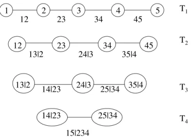
4Figure 1. A D-vine with 5 variables, 4 trees and 10 edges. Each edge may be may be associated with a pair-copula.
2.1. Vines
For high-dimensional distributions, there are a significant number of possible pair-copulae constructions. For example, as will be shown in Section 2.4, there are 240 different construc-tions for a five-dimensional density. To help organising them, Bedford and Cooke (2001b, 2002) have introduced a graphical model denotedthe regular vine. The class of regular vines is still very general and embraces a large number of possible pair-copula decompositions. Here, we concentrate on two special cases of regular vines; thecanonical vineand theD-vine
(Kurowicka and Cooke, 2004). Each model gives a specific way of decomposing the density. The specification may be given in form of a nested set of trees. Figure 1 shows the specifi-cation corresponding to a five-dimensional D-vine. It consists of four treesTj, j= 1, . . .4.
TreeTj has 6−j nodes and 5−j edges. Each edge corresponds to a pair-copula density
and the edge label corresponds to the subscript of the pair-copula density, e.g. edge 14|23 corresponds to the copula density c14|23(·). The whole decomposition is defined by the
n(n−1)/2 edges and the marginal densities of each variable. The nodes in treeTj are only
necessary for determining the labels of the edges in treeTj+1. As can be seen from Figure
1, two edges inTj, which become nodes inTj+1, are joined by an edge inTj+1 only if these
edges in Tj share a common node. Note that the tree structure is not strictly necessary
for applying the pair-copula methodology, but it helps identifying the different pair-copula decompositions.
Bedford and Cooke (2001b) give the density of ann-dimensional distribution in terms of a regular vine, which we specialise to a D-vine and a canonical vine. The density
f(x1, . . . , xn) corresponding to a D-vine may be written as n Y k=1 f(xk) n−1 Y j=1 n−j Y i=1 ci,i+j|i+1,...,i+j−1(F(xi|xi+1, . . . , xi+j−1), F(xi+j|xi+1, . . . , xi+j−1)), (8)
where indexj identifies the trees, while iruns over the edges in each tree.
In a D-vine, no node in any treeTj is connected to more than two edges. In a canonical
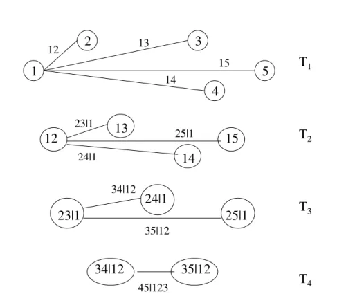
vine, each treeTj has a unique node that is connected to n−j edges. Figure 2 shows a
canonical vine with 5 variables. The n-dimensional density corresponding to a canonical vine is given by n Y k=1 f(xk) n−1 Y j=1 n−j Y i=1 cj,j+i|1,...,j−1(F(xj|x1, . . . , xj−1), F(xj+i|x1, . . . , xj−1)). (9)
T
1T
2T
3T
434|12 35|12
45|123
34|12
23|1
25|1
35|12
24|1
12
13
14
15
25|1
24|1
23|1
1
2
3
5
4
15
14
13
12
Figure 2. A canonical vine with 5 variables, 4 trees and 10 edges.
Fitting a canonical vine might be advantageous when a particular variable is known to be a key variable that governs interactions in the data set. In such a situation one may decide to locate this variable at the root of the canonical vine, as we have done with variable 1 in Figure 2. The notation of D-vines resembles independence graphs more than that of canonical vines.
2.2. Three variables
The general expression for both the canonical and the D-vine structures in the three-dimensional case is
f(x1, x2, x3) = f(x1)·f(x2)·f(x3)
· c12(F(x1), F(x2))·c23(F(x2), F(x3)) (10)
· c13|2(F(x1|x2), F(x3|x2)).
There are six ways of permuting x1, x2 and x3, in (10), but only three give different
decompositions. Moreover, each of the 3 decompositions is both a canonical vine and a D-vine.
2.3. Four variables
The four-dimensional canonical vine structure is generally expressed as f(x1, x2, x3, x4) = f(x1)·f(x2)·f(x3)·f(x4)
· c12(F(x1), F(x2))·c13(F(x1), F(x3))·c14(F(x1), F(x4))
· c23|1(F(x2|x1), F(x3|x1))·c24|1(F(x2|x1), F(x4|x1))
· c34|12(F(x3|x1, x2), F(x4|x1, x2)),
and the D-vine structure as
f(x1, x2, x3, x4) = f(x1)·f(x2)·f(x3)·f(x4)
· c12(F(x1), F(x2))·c23(F(x2), F(x3))·c34(F(x3), F(x4)) (11)
· c13|2(F(x1|x2), F(x3|x2))·c24|3(F(x2|x3), F(x4|x3))
· c14|23(F(x1|x2, x3), F(x4|x2, x3)).
In Appendix A we derive these expressions.
In total, there are 12 different D-vine decompositions and 12 different canonical vine decompositions, and none of the D-vine decompositions are equal to any of the canonical vine decompositions. There are no other possible regular vine decompositions. Hence, in the four-dimensional case there are 24 different possible pair-copula decompositions, 12 canonical vines and 12 D-vines.
2.4. Five variables
The general expression for the five-dimensional canonical vine structure is f(x1, x2, x3, x4, x5) = f(x1)·f(x2)·f(x3)·f(x4)·f(x5) · c12(F(x1), F(x2))·c13(F(x1), F(x3))·c14(F(x1), F(x4)) · c15(F(x1), F(x5))·c23|1(F(x2|x1), F(x3|x1)) · c24|1(F(x2|x1), F(x4|x1))·c25|1(F(x2|x1), F(x5|x1)) · c34|12(F(x3|x1, x2), F(x4|x1, x2))·c35|12(F(x3|x1, x2), F(x5|x1, x2)) · c45|123(F(x4|x1, x2, x3), F(x5|x1, x2, x3)),
and the general expression for the D-vine structure is f(x1, x2, x3, x4, x5) = f(x1)·f(x2)·f(x3)·f(x4)·f(x5) · c12(F(x1), F(x2))·c23(F(x2), F(x3))·c34(F(x3), F(x4)) · c45(F(x4), F(x5))·c13|2(F(x1|x2), F(x3|x2)) · c24|3(F(x2|x3), F(x4|x3))·c35|4(F(x3|x4), F(x5|x4)) · c14|23(F(x1|x2, x3), F(x4|x2, x3))·c25|34(F(x2|x3, x4), F(x5|x3, x4)) · c15|234(F(x1|x2, x4, x3), F(x5|x2, x4, x3)).
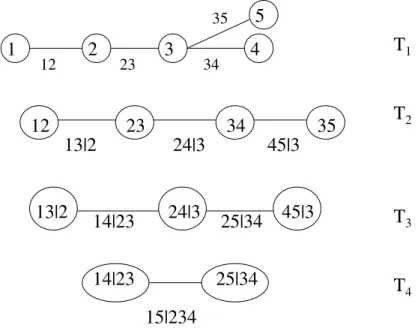
In the five-dimensional case there are regular vines that are neither canonical nor D-vines. One example is the following:
f12345(x1, x2, x3, x4, x5) = f1(x1)·f2(x2)·f3(x3)·f4(x4)·f5(x5) · c12(F1(x1), F2(x2))·c23(F2(x2), F3(x3))·c34(F3(x3), F4(x4)) · c35(F3(x3), F5(x5)) · c13|2 ¡ F1|2(x1|x2), F3|2(x3|x2)¢·c24|3(F2|3(x2|x3), F4|3(x4|x3)) · c45|3(F4|3(x4|x3), F5|3(x5|x3)) · c14|23(F1|23(x1|x2, x3), F4|23(x4|x2, x3)) · c25|34(F2|34(x2|x3, x4), F5|34(x5|x3, x4)) · c15|234(F1|234(x1|x2, x3, x4), F5|234(x5|x2, x3, x4)).
The corresponding structure is shown in Figure 3. In treeT1 node 3 has three neighbours;
2,4 and 5. Hence, this is not a D-vine, for which no node in any tree is connected to more than two edges. Moreover, it is not a canonical vine, since node 3 inT1 is connected to 3
edges instead of 4.
In total there are 60 different D-vines and 60 different canonical vines in the five-dimensional case, and none of the D-vines are equal to any of the canonical vines. In addition to the canonical and D-vines, there are also 120 other regular vines. Hence, in the five-dimensional case there are 240 different possible pair-copula decompositions, 60 canonical vines, 60 D-vines, and 120 other types of decompositions.
2.5. nvariables
Considering Figure 2 we see that the conditioning sets of the edgesin each of the trees T2, T3andT4are the same. For example inT3the conditioning set is always{12}. Extending
this idea to n nodes, we see that there are n choices for the conditioning set {i2} in T2,
n−1 choices for the conditioning set{i2, i3}inT3oncei2is chosen inT2. Finally, we have
3 choices for the conditioning set{in−1, in−2,· · ·, i2}when i2,· · · , in−2 are chosen before.
So all together we haven(n−1)· · ·3 = n2! different canonical vines onnnodes.
For an n-dimensional D-vine, there are n! choices to arrange the order in the tree T1.
Since we have undirected edges, i.e. cij|D=cji|Dfor all pairsi, jand arbitrary conditioning
sets for D-vines, we can reverse the order in the treeT1 for a D-vine without changing the
corresponding vine. Therefore we have only n2! different trees on the first level. Given a such a treeT1, the treesT2, T3,· · ·, Tn−1 are completely determined. This implies that the
number of distinct D-vines onnnodes is given by n! 2.
1 2 3 4
12 23 34 35
12 23 3413|2 24|3 45|3
13|2 24|3 45|3
14|23 25|34
14|23 25|34
15|234
T
1T
2T
3T
45
35Figure 3. A regular vine with 5 variables, 4 trees and 10 edges.
2.6. Multivariate Gaussian distribution
If the marginal distributionsf(xi) in (10) are standard normal, andc12(·),c23(·) andc13|2(·)
are bivariate Gaussian copula densities (see Appendix B.1) the resulting distribution is trivariate standard normal with the positive definite correlation matrix
1 ρ12 ρ13 ρ12 1 ρ23 ρ13 ρ23 1 .
Here ρ12 and ρ23 are the correlation parameters of copulae c12(·) andc23(·), respectively,
whileρ13is given by ρ13=ρ13|2 q 1−ρ2 12 q 1−ρ2 23+ρ12ρ23.
The correlation parameter of copula c13|2(·), ρ13|2, is called partial correlation, see e.g.
Kendall and Stuart (1967) for a definition. Note that it is only for the joint normal distri-bution that the partial and conditional correlations are equal (Morales et al., 2006). The meaning of partial correlation for non-normal variables is less clear.
3. Conditional independence and the pair-copula decomposition
Assuming conditional independence may reduce the number of levels of the pair-copula de-composition, and hence simplify the construction. Let us first consider the three-dimensional case again with the pair copula decomposition in (10). If we assume that X1 and X3 are
1 2
3 4
Figure 4. A conditional independence graph with 4 variables.
independent givenX2, we have thatc13|2(F(x1|x2), F(x3|x2)) = 1. Hence, the pair copula
decomposition in (10) simplifies to
f(x1, x2, x3) =f(x1)·f(x2)·f(x3)·c12(F(x1), F(x2))·c23(F(x2), F(x3)). (12)
In general, for any vector of variables V and two variables X, Y, it holds thatX and Y
are conditionally independent givenV if and only if
cxy|v
¡
Fx|v(x|v), Fy|v(y|v)
¢
= 1. (13)
As usual in hierarchical modelling, a model simplifies only if the initial factorisation of the joint density takes advantage of assumed conditional independence. For instance, if we use the decomposition f(x1, x2, x3) =f(x2|x1, x3)f(x1|x3)f(x3) in the case when X1 and
X3 are conditionally independent givenX2, all pair-copulae are needed.
If the conditional independence assumption is only made to simplify the model construc-tion, we may use the pair-copula decomposition to measure the approximation error intro-duced by this assumption. For example, take a four variable model, and assume conditional independence as expressed by the four variables in the conditional independence graph given in Figure 4. That is, variablesX1andX4are assumed to be conditionally independent given
X3andX2, and variablesX2andX3are assumed to be conditionally independent givenX1
andX4. If we choose the decomposition in (11), the termc14|23(F(x1|x2, x3), F(x4|x2, x3))
should be equal to one, and the approximation error introduced by the conditional inde-pendence assumption is given by the differencec14|23(F(x1|x2, x3), F(x4|x2, x3))−1.
4. Simulation from a pair-copulae decomposed model
Simulation from vines is briefly discussed in Bedford and Cooke (2001a), Bedford and Cooke (2001b), and Kurowicka and Cooke (2005). In this section we show that the simulation algorithms for canonical vines and D-vines are straightforward and simple to implement. In the rest of this paper we assume for simplicity that the margins of the distribution of interest are uniform.
The general algorithm for samplingndependent uniform [0,1] variables is common for the canonical and the D-vine: First, samplewi;i = 1;. . . n independent uniform on [0,1].
Then, set x1 = w1 x2 = F2−|11(w2|x1) x3 = F3−|11,2(w3|x1, x2) .. = .... xn = Fn−|11,2,...,n−1(wn|x1, . . . , xn−1). (14)
To determineF(xj|x1, x2, . . . , xj−1) for each j, we use the definition of the h-function in
(7) and the relationship in (6), recursively for both vine structures. However, choice of the vj variable in (6) is different for the canonical vines and D-vines. For the canonical vine we
always choose
F(xj|x1, x2, . . . , xj−1) =
∂ Cj,j−1|1,...j−2(F(xj|x1, . . . , xj−2), F(xj−1|x1, . . . , xj−2))
∂F(xj−1|x1, . . . , xj−2)
, while for the D-vine we choose
F(xj|x1, x2, . . . , xj−1) =
∂ Cj,1|2,...j−1(F(xj|x2, . . . , xj−1), F(x1|x2, . . . , xj−1))
∂F(x1|x2, . . . , xj−1) .
4.1. Sampling a canonical vine
Algorithm 1 gives the procedure for sampling from a canonical vine. The outer for-loop runs over the variables to be sampled. This loop consists of two other for-loops. In the first, theith variable is sampled, while in the other, the conditional distribution functions needed for sampling the (i+ 1)th variable are computed. To compute these conditional distribution functions, we use the h-function, defined by (7) in Section 2, repeatedly with previously computed conditional distribution functions,vi,j=F(xi|x1, ...xj−1), as the first
two arguments. The last argument of the h-function, Θj,i, is the set of parameters of the
corresponding copula densitycj,j+i|1,...,j−1(·).
4.2. Sampling a D-vine
Algorithm 2 gives the procedure for sampling from the D-vine. It also consists of one main for-loop containing one for-loop for sampling the variables and one for-loop for computing the needed conditional distribution functions. However, this algorithm is computationally less efficient than that for the canonical vine, as the number of conditional distribution functions to be computed when simulatingnvariables is (n−2)2 for the D-vine, while it
is (n−2)(n−1)/2 for the canonical vine. Again the h-function is defined by (7) in Section 2, but here Θj,iis the set of parameters of the copula densityci,i+j|i+1,...,i+j−1(·).
4.3. Sampling a 3-dimensional vine
In this section, we describe how to sample from a 3-dimensional canonical vine. Since all decompositions in the 3-dimensional case are both a canonical vine and a D-vine, the resulting sample will also be a sample from a D-vine.
First, sample wi;i = 1,2,3 independent uniform on [0,1]. Then, x1 = w1.
Algorithm 1Simulation algorithm for a canonical vine. Generates one samplex1, . . . xn from the vine.
Samplewi;i= 1;. . . nindependent uniform on [0,1].
x1=v1,1=w1 fori←2,3, . . . , n vi,1=wi fork←i−1, i−2, . . . ,1 vi,1=h−1(vi,1, vk,k,Θk,i−k) end for xi=vi,1 if i==nthen Stop end if forj ←1,2, . . . , i−1
vi,j+1=h(vi,j, vj,j,Θj,i−j)
end for end for
Algorithm 2Simulation algorithm for D-vine. Generates one samplex1, . . . xn from the vine.
Samplewi;i= 1;. . . nindependent uniform on [0,1].
x1=v1,1=w1 x2=v2,1=h−1(w2, v1,1,Θ1,1) v2,2=h(v1,1, v2,1,Θ1,1) fori←3,4, . . . n vi,1=wi fork←i−1, i−2, . . . ,2 vi,1=h−1(vi,1, vi−1,2k−2,Θk,i−k) end for vi,1=h−1(vi,1, vi−1,1,Θ1,i−1) xi=vi,1 if i==nthen Stop end if vi,2=h(vi−1,1, vi,1,Θ1,i−1) vi,3=h(vi,1, vi−1,1,Θ1,i−1) if i >3 then forj←2,3, . . . , i−2 vi,2j =h(vi−1,2j−2, vi,2j−1,Θj,i−j) vi,2j+1=h(vi,2j−1, vi−1,2j−2,Θj,i−j) end for end if vi,2i−2=h(vi−1,2i−4, vi,2i−3,Θi−1,1) end for
F(x3|x1, x2) = h(F(x3|x1), F(x2|x1),Θ21) = h(h(x3, x1,Θ12), h(x2, x1,Θ11),Θ21),
mean-ing thatx3=h−1¡h−1(w3, h(x2, x1,Θ11),Θ21), x1,Θ12¢.
5. Inference for a speci£ed pair-copula decomposition
In this section we describe how the parameters of the canonical vine density given by (9) or D-vine density given by (8) can be estimated by maximum likelihood. Inference for a general regular vine (like the one in Figure 3) is also feasible, but the algorithm is not as straightforward. Assume that we observe n variables at T time points. Let
xi = (xi,1, . . . , xi,T);i = 1, . . . n denote the data set. Here, each random variable Xi,t
is assumed to be uniform in [0,1]. We assume for simplicity that the T observations of each variable are independent over time. This is not a necessary assumption, as stochastic dependencies and time series dynamics can easily be incorporated.
5.1. Inference for a canonical vine
For the canonical vine, the log-likelihood is given by
n−1 X j=1 n−j X i=1 T X t=1 log¡ cj,j+i|1,...,j−1(F(xj,t|x1,t, . . . , xj−1,t), F(xj+i,t|x1,t, . . . , xj−1,t))¢. (15)
For each copula in the sum (15) there is at least one parameter to be determined. The number depends on which copula type is used. As before, the conditional distributions F(xj,t|x1,t, . . . , xj−1,t) and F(xj+i,t|x1,t, . . . , xj−1,t) are determined using the relationship
in (6) and the definition of the h-function in (7). The log-likelihood must be numerically maximised over all parameters.
Algorithm 3 evaluates the likelihood for the canonical vine. The outer for-loop corre-sponds to the outer sum in (15). This for-loop consists in turn of two other for-loops. The first of these corresponds to the sum overiin (15). In the other, the conditional distribution functions needed for the next run of the outer for-loop are computed. Here Θj,i is the set
of parameters of the corresponding copula densitycj,j+i|1,...,j−1(·),h(·) is given by (7), and
element tof vj,i is vj,i,t=F(xi+j,t|x1,t, . . . , xj,t). Further,L(x,v,Θ) is the log-likelihood
of the chosen bivariate copula with parameters Θ given the data vectorsxandv. That is,
L(x,v,Θ) =
T
X
t=1
log (c(xt, vt,Θ)), (16)
wherec(u, v,Θ) is the density of the bivariate copula with parameters Θ.
Starting values of the parameters needed in the numerical maximisation of the log-likelihood may be determined as follows:
(a) Estimate the parameters of the copulae in tree 1 from the original data
(b) Compute observations (i.e. conditional distrubution functions) for tree 2 using the copula parameters from tree 1 and theh(·) function.
(c) Estimate the parameters of the copulae in tree 2 using the observations from (b). (d) Compute observations for tree 3 using the copula parameters at level 2 and theh(·)
function.
Algorithm 3Likelihood evaluation for canonical vine log-likelihood = 0 fori←1,2, . . . , n v0,i=xi. end for forj←1,2, . . . , n−1 fori←1,2, . . . , n−j
log-likelihood = log-likelihood +L(vj−1,1,vj−1,i+1,Θj,i)
end for if j==n−1then Stop end if fori←1,2, . . . , n−j vj,i=h(vj−1,i+1,vj−1,1,Θj,i) end for end for (f) etc.
Note that each estimation here is easy to perform, since the data set is only of dimension 2.
5.2. Inference for a D-vine
For the D-vine, the log-likelihood is given by
n−1 X j=1 n−j X i=1 T X t=1 log¡
ci,i+j|i+1,...,i+j−1(F(xi,t|xi+1,t, . . . , xi+j−1,t), F(xi+j,t|xi+1,t, . . . , xi+j−1,t))
¢
. (17) The D-vine log-likelihood must also be numerically optimised. Algorithm 4 evaluates the likelihood. Θj,i is the set of parameters of copula densityci,i+j|i+1,...,i+j−1(·).
5.3. Inference for a 3 variable model
In the special case of a 3-dimensional data set withU[0,1] distributed variables, (15) reduces to
T
X
t=1
£
logc12(x2,t, x1,t,Θ11) + logc23(x2,t, x3,t,Θ12) + logc13|2(v1,t, v2,t,Θ21)¤, (18)
where
v1,t=F(x1,t|x2,t) =h(x1,t, x2,t,Θ11)
and
v2,t=F(x3,t|x2,t) =h(x3,t, x2,t,Θ12)
The parameters to be estimated are Θ = (Θ11,Θ12,Θ21), where Θj,i is the set of
Algorithm 4Likelihood evaluation for a D-vine log-likelihood = 0 fori= 1,2, . . . , n v0,i=xi. end for fori= 1,2, . . . , n−1 log-likelihood=log-likelihood+L(v0,i,v0,i+1,Θ1,i) end for v1,1=h(v0,1,v0,2,Θ1,1) fork= 1,2, . . . , n−3 v1,2k =h(v0,k+2,v0,k+1,Θ1,k+1) v1,2k+1=h(v0,k+1,v0,k+2,Θ1,k+1) end for v1,2n−4=h(v0,n,v0,n−1,Θ1,n−1) forj= 2, . . . , n−1 fori= 1,2, . . . , n−j log-likelihood=log-likelihood+L(vj−1,2i−1,vj−1,2i,Θj,i) end for if j==n−1then Stop end if vj,1=h(vj−1,1,vj−1,2,Θj,1) if n >4 then fori= 1,2, . . . , n−j−2 vj,2i=h(vj−1,2i+2,vj−1,2i+1,Θj,i+1) vj,2i+1=h(vj−1,2i+1,vj−1,2i+2,Θj,i+1) end for end if vj,2n−2j−2=h(vj−1,2n−2j,vj−1,2n−2j−1,Θj,n−j) end for
described in Section 5.1, we first estimate the parameters of the three copulae involved by a sequential procedure, and then we maximize the full log-likelihood using the parameters obtained from the stepwise procedure as starting values.
6. A catalogue of some pair-copulae models
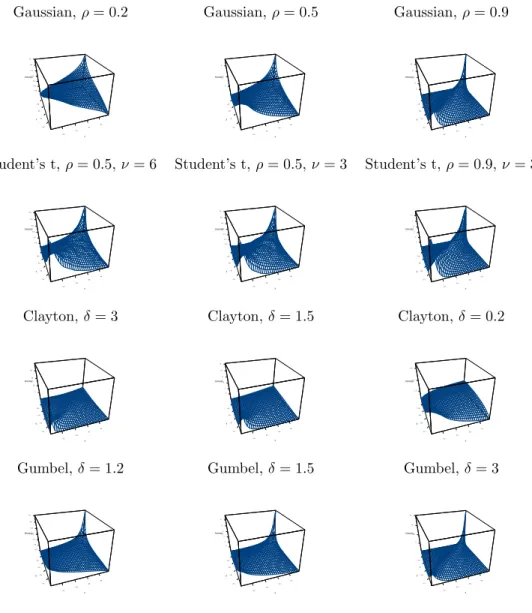
Pair-copulae are basic building blocs for constructing multivariate models. In this section we present four of the most common pair-copulae. We discuss in particular their param-eterisation and the type of pair dependence they capture. See Joe (1997) for an overview of other copulae. Tail dependence properties are particularly important in many applica-tions that rely on non-normal multivariate families (Joe, 1996). The four bivariate copulae in question are the Gaussian, the Student’s t, the Clayton and the Gumbel copula. The first two are copulae of normal mixture distributions. They are so-called implicit copulae because they do not have a simple closed form. Clayton and Gumbel are Archimedean copulae, for which the distribution function has a simple closed form. These four types of copulae have different strength of dependence in the tails of the bivariate distribution. This can be represented by the probability that the first variable exceeds itsq-quantile, given that the other exceeds its ownq-quantile. The limiting probability, asq goes to infinity, is called theupper tail dependence coefficient (Embrechts et al., 2001) , and a copula is said to be upper tail dependent if this limit is not zero. Thelower tail dependence coefficient
is defined analogously. The Clayton copula is lower tail dependent, but not upper. The Gumbel copula is upper tail dependent, but not lower. The Student’s t-copula is both lower and upper tail dependent, while the Gaussian is neither lower nor upper tail dependent.
In Appendix B we give three important formulas for each of these four pair copulae; the density, the h-function and the inverse of the h-function. The Gaussian, Clayton and Gumbel pair-copulae have one parameter, while the Student’s-t pair-copula has two. The additional parameter of the latter is the degrees of freedom, that controls the strength of dependence in the tails of the bivariate distribution. The Student’s t-copula allows for joint extreme events, either in both bivariate tails or none of them. If one believes that the variables are only lower tail dependent, then the Clayton copula, which is an asymmetric copula, exhibiting greater dependence in the negative tail than in the positive, might be a better choice. The Gumbel copula is also an asymmetric copula, but it is exhibiting greater dependence in the positive tail than in the negative. Figure 5 shows the densities of the four copulae for three different parameter settings.
For all these four pair-copulae the h-function is given by an explicit analytical expression, see Appendix B. This expression can be analytically inverted for all pair-copulae except for the Gumbel, where numerical inversion is necessary. Explicit availability of the h-functions and their inverse is very important for the efficiency of our estimation procedures.
7. Model selection
In Section 5 we described how to do inference for a specific pair-copula decomposition. However, this is only a part of the full estimation problem. Full inference for a pair-copula decomposition should in principle consider (a) the selection of a specific factorisation, (b) the choice of pair-copula types, and (c) the estimation of the copula parameters. For smaller dimensions (say 3 and 4), one may estimate the parameters of all possible decompositions using the procedure described in Section 5 and compare the resulting log-likelihoods. This
Gaussian,ρ= 0.2 Gaussian,ρ= 0.5 Gaussian,ρ= 0.9 0.2 0.4 0.6 0.8 0.2 0.4 0.6 0.8 0.6 0.8 1.0 1.2 1.4 1.6 1.8 x y Density 0.2 0.4 0.6 0.8 0.2 0.4 0.6 0.8 1 2 3 x y Density 0.2 0.4 0.6 0.8 0.2 0.4 0.6 0.8 2 4 6 8 10 x y Density
Student’s t,ρ= 0.5,ν= 6 Student’s t,ρ= 0.5,ν = 3 Student’s t,ρ= 0.9,ν= 3
0.2 0.4 0.6 0.8 0.2 0.4 0.6 0.8 0.5 1.0 1.5 2.0 2.5 3.0 x y Density 0.2 0.4 0.6 0.8 0.2 0.4 0.6 0.8 0.5 1.0 1.5 2.0 2.5 3.0 3.5 x y Density 0.2 0.4 0.6 0.8 0.2 0.4 0.6 0.8 1 2 3 4 5 6 x y Density
Clayton,δ= 3 Clayton,δ= 1.5 Clayton,δ= 0.2
0.2 0.4 0.6 0.8 0.2 0.4 0.6 0.8 5 10 15 20 x y Density 0.2 0.4 0.6 0.8 0.2 0.4 0.6 0.8 2 4 6 8 10 12 x y Density 0.2 0.4 0.6 0.8 0.2 0.4 0.6 0.8 1.0 1.5 2.0 x y Density
Gumbel,δ= 1.2 Gumbel,δ= 1.5 Gumbel,δ= 3
0.2 0.4 0.6 0.8 0.2 0.4 0.6 0.8 0.5 1.0 1.5 2.0 2.5 3.0 3.5 x y Density 0.2 0.4 0.6 0.8 0.2 0.4 0.6 0.8 1 2 3 4 5 6 x y Density 0.2 0.4 0.6 0.8 0.2 0.4 0.6 0.8 5 10 15 20 x y Density
Figure 5. 3D surface plot of bivariate density for Gaussian, Student’s t, Clayton and Gumbel copulae, with three different parameter settings.
is in practice infeasible for higher dimensions, since the number of possible decompositions increases very rapidly with the dimension of the data set, as shown in Section 2. One should instead consider which bivariate relationships that are most important to model correctly, and let this determine which decomposition(s) to estimate. D-vines are more flexible than canonical vines, since for the canonical vines we specify the relationships between one specific pilot variable and the others, while in the D-vine structure we can select more freely which pairs to model.
Given data and an assumed pair-copula decomposition, it is necessary to specify the parametric shape of each pair-copula. For example, for the decomposition in Section 5.3 we need to decide which copula type to use forC12(·,·), C23(·,·) andC13|2(·,·) (for instance
among the ones described in Section 6). The pair-copulae do not have to belong to the same family. The resulting multivariate distribution will be valid if we choose for each pair of variables the parametric copula that best fits the data. If we choose not to stay in one predefined class, we need a way of determining which copula to use for each pair of (transformed) observations. We propose to use a modified version of the sequential estimation procedure outlined in Section 5.1:
(a) Determine which copula types to use in tree 1 by plotting the original data, or by applying a Goodness-of-Fit (GoF) test, see Section 7.1.
(b) Estimate the parameters of the selected copulae using the original data.
(c) Transform observations as required for tree 2, using the copula parameters from tree 1 and theh(·) function as shown in Sections 5.1 and 5.2.
(d) Determine which copula types to use in tree 2 in the same way as in tree 1. (e) Iterate.
The observations used to select the copulae at a specific level depend on the specific pair-copulae chosen up-stream in the decomposition. This selection mechanism does not guaran-tee an globally optimal fit. Having determined the appropriate parametric shapes for each copulae, one may use the procedures in Section 5 to estimate their parameters.
7.1. Godness-of-£t
To verify whether the dependency structure of a data set is appropriately modelled by a chosen pair-copula decomposition, we need a goodness-of-fit (GOF) test. GOF tests for dependency structures are basically special cases of the more general problem of testing multivariate densities. However, it is more technically complicated as the univariate dis-tribution functions are unknown. Hence, despite an obvious need for such tests in applied work, relatively little is known about their properties, and there is still no recommended method agreed upon.
Of the tests that have been proposed, quite a few are based on the probability integral transform (PIT) of Rosenblatt (1952). The PIT converts a set of dependent variables into a new set of variables which are independent and uniform under the null hypothesis that the data originate from a given multivariate distribution. The technique is somehow the inverse of simulation and is defined as follows.
Let X = (X1, . . . Xn) denote a random vector with marginal distributions Fi(xi) and
asT(X) = (T1(X1), . . . Tn(Xn)), whereTi(Xi) is given by: T1(X1) = F1(x1) T2(X2) = F2|1(x2|x1) · = · (19) · = · Tn(Xn) = Fn|1,...n−1(xn|x1, . . . xn−1). (20) The random variablesZi =Ti(Xi), i= 1, . . . nare independent and uniformly distributed on
[0,1]nunder the null hypothesis thatXcomes from the multivariate model used to compute
the PIT ofX. It is relatively easy to specialise the PIT to the pair-copula decomposition.
Algorithms 5 and 6 give the procedures for a canonical vine and a D-vine, respectively.
Algorithm 5PIT algorithm for a canonical vine
fort←1,2, . . . , T z1,t=x1,t
fori←2,3, . . . , n zi,t=xi,t
forj←1,2, . . . i−1 zi,t =h(zi,t, zj,t,Θj,i−j)
end for end for end for
Having performed the probability integral transform, the next step is to verify whether the resulting variables really are independent and uniform in [0,1]. The most common approach is to compute S = Pn i=1 ¡ Φ−1(Z i) ¢2
, and test whether the observed values of S come from a chi-square distribution withn degrees of freedom. The Anderson-Darling goodness-of-fit test may be applied for the latter, see e.g. Breymann et al. (2003).
8. Application: Financial returns
8.1. Data set
In this section, we study four time series of daily data: the Norwegian stock index (TOTX), the MSCI world stock index, the Norwegian bond index (BRIX) and the SSBWG hedged bond index, for the period from 04.01.1999 to 08.07.2003. Figure 6 shows the log-returns of each pair of assets. The four variables will be denotedT,M,B andS.
We want to compare a four-dimensional pair-copula decomposition with Student’s t-copulae for all pairs with the four-dimensional Student’s t-copula. Then-dimensional Stu-dent’s t-copula has been used repeatedly for modelling multivariate financial return data. A number of papers, such as Mashal and Zeevi (2002), have shown that the fit of this copula is generally superior to that of other n-dimensional copulae for such data. However, the Students’s t-copula has only one parameter for modelling tail dependence, independent of dimension. Hence, if the tail dependence of different pairs of risk factors in a portfolio are very different, we believe the pair-copula decomposition with Student’s t-copulae for all
Algorithm 6PIT algorithm for a D-vine fort←1,2, . . . , T z1,t=x1,t z2,t=h(x2,t, x1,t,Θ1,1) v2,1=x2,t v2,2=h(x1,t, x2,t,Θ1,1) fori←3,4, . . . n zi,t=h(xi,t, xi−1,t,Θ1,i−1) forj←2,3, . . . i−1
zi,t =h(zi,t, vi−1,2(j−1),Θj,i−j)
end for if i==nthen Stop end if vi,1=xi,t vi,2=h(vi−1,1, vi,1,Θ1,i−1) vi,3=h(vi,1, vi−1,1,Θ1,i−1) forj←1,2, . . . , i−3 vi,2j+2=h(vi−1,2j, vi,2j+1,Θj+1,i−j−1) vi,2j+3=h(vi,2j+1, vi−1,2j,Θj+1,i−j−1) end for vi,2i−2=h(vi−1,2i−4, vi,2i−3,Θi−1,1) end for end for International bonds International stocks -0.010 -0.005 0.0 0.005 -0.04 -0.02 0.0 0.02 0.04 International bonds Norwegian stocks -0.010 -0.005 0.0 0.005 -0.06 -0.02 0.02 International bonds Norwegian bonds -0.010 -0.005 0.0 0.005 -0.005 0.0 0.005 0.010 International stocks Norwegian stocks -0.04 -0.02 0.0 0.02 0.04 -0.06 -0.02 0.02 International stocks Norwegian bonds -0.04 -0.02 0.0 0.02 0.04 -0.005 0.0 0.005 0.010 Norwegian stocks Norwegian bonds -0.06 -0.02 0.02 -0.005 0.0 0.005 0.010
S
SMM
MTT
TBB
SM
MT
TB
ST|M MB|T
ST|M
MB|T
SB|MT
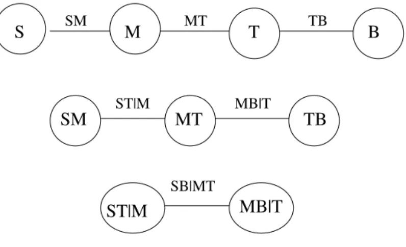
Figure 7. Selected D-vine structure for the data set in Section 8.1.
pairs to describe the dependence structure of the risk factors better. Since we are mainly interested in estimating the dependence structure of the risk factors, the original data vec-tors are converted to uniform variables using the empirical distribution functions before further modelling.
8.2. Selecting an appropriate pair-copula decomposition
Having decided to use Student’s t-copulae for all pairs of the decomposition, the next step is to choose the most appropriate ordering of the risk factors. This is done by first fitting a bivariate Student’s t-copula to each pair of risk factors, obtaining an estimated degree of freedom for each pair. The estimation of the Student’s t-copula parameters requires numerical optimisation of the log-likelihood function, see for instance Mashal and Zeevi (2002) or Demarta and McNeil (2005).
Having fitted a bivariate Student’s t-copula to each pair, the risk factors are ordered such that the three copulae to be fitted in tree 1 in the pair-copula decomposition are those corresponding to the three smallest numbers of degrees of freedom. A low number of degrees of freedom indicates strong dependence. The number of degrees of freedom parameters from our case are shown in Table 1. The dependence is strongest between international bonds and stocks (S and M), international and Norwegian stocks (M and T), and Norwegian stocks and bonds (T and B). Hence, we want to fit the copulaeCS,M,CM,T andCT,Bin tree 1 of
the vine. This means that we can not use a canonical vine, since there is no pilot variable. However, using a D-vine specification with the nodesS, M, T, andB in the listed order, gives the three above-mentioned copulae at level 1. See Figure 7 for the whole D-vine structure in this case.
8.3. Inference
The parameters of the D-vine are estimated using the algorithm in Section 5.2. For each pair-copula, the log-likelihood is computed using (16) and the density and the h-function
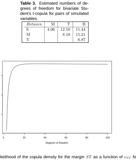
grees of freedom for bivariate Stu-dent’s t-copula for pairs of variables.
Between M T B
S 4.11 32.74 9.98
M 8.03 13.53
T 7.96
Table 2. Estimated parameters for four-dimensional pair-copula decomposition.
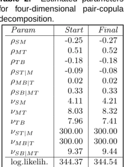
Param Start Final
ρSM -0.25 -0.27 ρM T 0.51 0.52 ρT B -0.18 -0.18 ρST|M -0.09 -0.08 ρM B|T 0.02 0.02 ρSB|M T 0.33 0.33 νSM 4.11 4.21 νM T 8.03 8.32 νT B 7.96 7.41 νST|M 300.00 300.00 νM B|T 300.00 300.00 νSB|M T 9.37 9.44 log.likelih. 344.37 344.54
for the Student’s t-copula given in Appendix B.2.
Table 2 shows the starting values obtained using the sequential estimation procedure (left column), and the final parameter values together with the corresponding log-likelihood values. In the numerical search for the degrees of freedom parameter we have used 300 as the maximum value. As can be seen from the table, the likelihood slightly increases when estimating all parameters simultaneously. The Akaike’s Information Criterion (AIC) for the final model is -665.08. The p-value for the goodness-of-fit test described in Section 7.1 was 0.70, meaning that we cannot reject the null hypothesis of a D-vine. It should be noted that using the empirical distribution functions to convert the original data vectors to uniform variables before fitting the dependency structure, will affect the critical values of this test in a complicated, non-trivial way. This is still an unsolved problem, not only for a pair-copula decomposition, but for copulae in general.
8.4. Validation by simulation
Having estimated the pair-copula decomposition, it is interesting to investigate the bivari-ate distributions of the pairs of variables which were not explicitly modelled in the decom-position. We sample from the estimated pair-copula decomposed model, with estimated parameters as above, and check if simulated values and observed data have similar features. We used the simulation procedure described in Section 4.2 and the h-function and its inverse given in Section B.2 to generate a set of 10,000 samples from the estimated pair-copula decomposition. Then, we estimated pairwise Student’s t-pair-copulae for all bivariate margins. The results are shown in Table 3. Comparing these to the ones in Table 1 we see
Table 3. Estimated numbers of de-grees of freedom for bivariate Stu-dent’s t-copula for pairs of simulated variables. Between M T B S 4.06 12.10 11.44 M 8.10 15.21 T 6.87 Degrees of freedom log-likelihood 0 20 40 60 80 100 0 10 20
Figure 8. The log-likelihood of the copula density for the marginST as a function ofνST forρST
£xed to -0.21.
that except for the pairS, T, the numbers are similar, indicating that all dependencies are quite well captured, also those that are not directly modelled.
In Figure 8, we show the log-likelihood of the pair-copula density for the pair S, T as a function ofνST, forρST fixed to -0.21. As can be seen from the figure, the likelihood is
very flat for a large range ofνST values, meaning that the difference betweenνST = 12.10
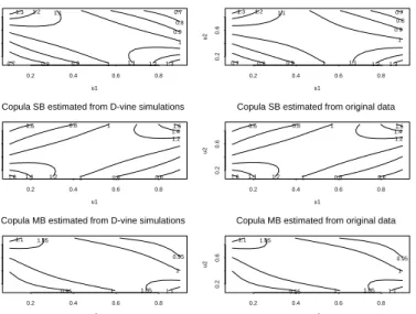
andνST = 32.74 is not as large as it may seem at first sight. This is verified by Figure 9,
which shows the contours of the densities of the copulae for the pairsS, T,S, B, andM, B, estimated both from the simulated D-vine and from the original data. The plots in the two columns are very similar.
8.5. Comparison with the four-dimensional Student’s t-copula
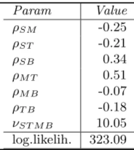
In this section we compare the results obtained with the pair-copula decomposition from Section 8.3 with those obtained with a four-dimensional Student’s t-copula. The parameters of the Student’s t-copula are estimated using the method described in Mashal and Zeevi (2002) and (Demarta and McNeil, 2005). They are shown in Table 4. The AIC for this model is -632.18, i.e. higher than that for the pair-copulae decomposition. Further, all
condi-u1 u2 0.2 0.4 0.6 0.8 0.2 0.6 0.7 0.7 0.8 0.8 0.9 0.9 1 1 1.1 1.1 1.2 1.2 1.3 1.3
Copula ST estimated from D-vine simulations
u1 u2 0.2 0.4 0.6 0.8 0.2 0.6 0.7 0.7 0.8 0.8 0.9 0.9 1 1 1.1 1.1 1.2 1.2 1.3 1.3
Copula ST estimated from original data
u1 u2 0.2 0.4 0.6 0.8 0.2 0.6 0.6 0.6 0.8 0.8 1 1 1.2 1.2 1.4 1.4 1.6 1.6
Copula SB estimated from D-vine simulations
u1 u2 0.2 0.4 0.6 0.8 0.2 0.6 0.6 0.6 0.8 0.8 1 1 1.2 1.2 1.4 1.4 1.6 1.6
Copula SB estimated from original data
u1 u2 0.2 0.4 0.6 0.8 0.2 0.6 0.95 0.95 1 1 1.05 1.05 1.1 1.1
Copula MB estimated from D-vine simulations
u1 u2 0.2 0.4 0.6 0.8 0.2 0.6 0.95 0.95 1 1 1.05 1.05 1.1 1.1
Copula MB estimated from original data
Figure 9. Contours of the densities of the copulae for the bivariate marginsST, SB, and M B, estimated both from the simulated D-vine and from the original data.
tional distributions of a multivariate Students’s t-distribution are Students’s t-distributions. Hence, then-dimensional Student’s t-copula is a special case of an n-dimensional D-vine with the needed pairwise copulae in the D-vine structure set to the corresponding condi-tional bivariate distributions of the multivariate Student’s t-distribution. Therefore, the four-dimensional Students’s t-copula is nested within the considered D-vine structure and the likelihood ratio test statistic is 344.54-323.09=21.45 with 12-7=5 degrees of freedom. This yields a p-value of 0.0007 and shows that the 4 dimensional Student’s t-copula can be rejected in favour of the D-vine.
To illustrate the difference between the four-dimensional Students’s t-copula and the four-dimensional pair-copula decomposition, we have computed the tail dependence coeffi-cients for the three bivariate margins SM, M T andT B for both structures. See Section 6 for the definition of the upper and lower tail dependence coefficients. For the Student’s t-copula, the two coefficients are equal and given by (Embrechts et al., 2001)
λl(X, Y) =λu(X, Y) = 2tν+1 µ −√ν+ 1 r 1−ρ 1 +ρ ¶ ,
where tν+1 denotes the distribution function of a univariate Student’s t-distribution with
ν + 1 degrees of freedom. Table 5 shows the tail dependency coefficients for the three margins and both structures. For the bivariate marginSM, the value for the pair-copula distribution is 29 times higher than the corresponding one for the Student’s t-copula, and it is also significantly higher for the two other bivariate margins. For a trader holding a portfolio of international stocks and bonds, the practical implication of this difference in tail dependence is that the probability of observerving a large portfolio loss is much higher for the four-dimensional pair-copula decomposition that it is for the four-dimensional Student’s t-copula.
Table 4. Estimated parameters for four-dimensional Student’s t-copula. Param Value ρSM -0.25 ρST -0.21 ρSB 0.34 ρM T 0.51 ρM B -0.07 ρT B -0.18 νST M B 10.05 log.likelih. 323.09
Table 5. Tail dependence coef£cients.
Margin Pair-copula decomp. Student’s t-copula
SM 0.029 0.001
M T 0.119 0.086
T B 0.008 0.002
8.6. Pair-copula decomposition with copulae from different families
In this section we investigate whether we would get an even better fit for our data set if we allowed the pair-copulae in the decomposition defined by Figure 7 to come from different families. Figure 10 shows the data sets used to estimate the six pair-copulae in the decomposition described in Sections 8.2 and 8.3. The three scatter plots in the upper row correspond to the three bivariate marginsSM,M T andT B. The data clustering in the two opposite corners of these plots is a strong indication of both upper and lower tail dependence, meaning that the Student’s t-copula is an appropriate choice. In the two leftmost scatter plots in the lower row, the data seems to have no tail dependence and the two margins also appear to be uncorrelated. This is in accordance with the parameters estimated for these data sets, ρST|M, ρM B|T, νST|M, νM B|T, shown in Table 2. The correlation parameters
are very close to 0 and the degrees of freedom parameters are very large, meaning that the two variables constituting each pair are close to being independent. If so, cST|M(·) and
cM B|T(·) are both 1, which means that the pair-copula construction defined by Figure 7
may be simplified to
cSM(xS, xM)cM T(xM, xT)cT B(xT, xB)cSB|M T(F(xS|xM), F(xB|xT)).
In the scatter plot in the lower right corner of the figure, there seems to be data clustering in the lower left corner, but not in the upper right. This indicates that the Clayton copula might be a better choice than the Student’s t-copula, since it has lower tail dependence, but not upper. Hence, we have fitted the Clayton copula to this data set. The parameter was estimated to δ = 0.425. The likelihood of the Clayton copula is lower than that of the Student’s t-copula (59.86 vs. 68.62). However, since the two copulae are non-nested we cannot really compare the likelihoods. Instead we have used the procedure suggested by Genest and Rivest (1993) for identifying the appropriate copula. According to this procedure, we examine the degree of closeness of the parametric and non-parametric versions of the distribution functionK(z), defined by
S M 0.0 0.2 0.4 0.6 0.8 1.0 0.0 0.2 0.4 0.6 0.8 1.0 M T 0.0 0.2 0.4 0.6 0.8 1.0 0.0 0.2 0.4 0.6 0.8 1.0 T B 0.0 0.2 0.4 0.6 0.8 1.0 0.0 0.2 0.4 0.6 0.8 1.0 F(S|M) F(T|M) 0.0 0.2 0.4 0.6 0.8 1.0 0.0 0.2 0.4 0.6 0.8 1.0 F(M|T) F(B|T) 0.0 0.2 0.4 0.6 0.8 1.0 0.0 0.2 0.4 0.6 0.8 1.0 F(S|MT) F(B|MT) 0.0 0.2 0.4 0.6 0.8 1.0 0.0 0.2 0.4 0.6 0.8 1.0
Figure 10. The data sets used to estimate the six pair-copulae in the decomposition described in Sections 8.2 and 8.3.
For Archimedean copulae,K(z) is given by an explicit expression, while for the Student’s t-copula is has to be numerically derived. In Figure 11 we have plotted the quantiles of the non-parametric and parametric estimates ofK(z). The solid line corresponds to the case where the quantiles are equal, the dashed line to the Clayton copula, and the dotted line to the Student’s t-copula having parametersρSB|M T and νSB|M T given in Table 2. Since
it is difficult to distinguish the different lines in Figure 11, we have also made a plot of the difference between the parametric and the non-parametricK(z) for the two copulae, shown in Figure 12. The solid line corresponds to the Clayton copula and the dotted line to the Student’s t-copula. As can be seen from this figure, the quantiles of the Student’s t-copula are closer to the non-parametric quantiles than those of the Clayton copula. Hence, the pair-copula decomposition with Student’s t-copulae for all pairs remains the best choice for our data set.
9. Conclusions
We have shown how multivariate data exhibiting complex patterns of dependence in the tails can be modelled using pair-copulae. We have developed algorithms that allow infer-ence on the parameters of the pair-copulae on the various levels of the construction. This
Non-parametric K(z) Parametric K(z) 0.0 0.2 0.4 0.6 0.8 1.0 0.0 0.2 0.4 0.6 0.8 1.0
Figure 11. QQ-plot corresponding to the non-parametric and parametric estimates ofK(z). The solid line corresponds to the case where the quantiles are equal, the dashed line to the Clayton copula, and the dotted line to the Student’s t-copula having parametersρSB|M T andνSB|M T given
in Table 2. Non-parametric K(z) Parametric K(z)-Non-parametric K(z) 0.0 0.2 0.4 0.6 0.8 1.0 -0.02 -0.01 0.0 0.01 0.02 0.03
Figure 12. The difference between the non-parametric and parametric estimates of K(z). The solid line corresponds to the Clayton copula, and the dotted line to the Student’s t-copula having parametersρSB|M T andνSB|M T given in Table 2.
construction is hierarchical in nature, the various levels standing for growing conditioning sets, incorporating more variables. This differs from traditional hierarchical models, where levels depict conditional independence. Pair-copulae are simple building blocs, which can be compared to pairwise interaction potentials or cliques in Gibbs fields.
While we have assumed that the observations of the multivariate data are independent, this is not necessary. Pair-copula models can be built and estimated whenever there exists a likelihood function for the data, for example for ARMA or ARCH/GARCH. In fact, various forms of pseudo-maximum likelihood (Bollerslev and Wooldridge, 1992) can also be used instead of full likelihoods. Missing values are acceptable, though likelihoods become more complex, as in any other model. Bayesian versions of inference are easy to imagine, as there is no difficulty in adding priors on the parameters of the pair-copulae. One may also put priors on the choice of pairs to match. Posterior estimates will then substitute maximum likelihood ones.
Further research is needed to produce better comparison methods between alternative pair-copulae and between alternative decompositions. More powerful goodness-of-fit tests for bivariate models are crucial for the construction of an unsupervised algorithm that explores the large space of possible pair-copulae models. This however remains a central aim, since there is an increasing tendency to collect huge quantities of multivariate and dense observations, requiring automatic inferential methods.
Acknowledgements
This work is sponsored by the Norwegian fund Finansmarkedsfondet and the Norwegian Re-search Council. Claudia Czado is also supported by the Deutsche Forschungsgemainschaft, Sonderforschungsbereich 386, Statistical Analysis of discrete structures. The authors ac-knowledge the support of colleagues at the Norwegian Computing Center, in particular Daniel Berg and Ingrid Hobæk Haff.
References
Bedford, T. and R. M. Cooke (2001a). Monte Carlo simulation of vine dependent random variables for applications in uncertainty analysis. In 2001 Proceedings of ESREL2001,
Turin, Italy.
Bedford, T. and R. M. Cooke (2001b). Probability density decomposition for conditionally dependent random variables modeled by vines. Annals of Mathematics and Artificial
Intelligence 32, 245–268.
Bedford, T. and R. M. Cooke (2002). Vines - a new graphical model for dependent random variables. Annals of Statistics 30(4), 1031–1068.
Bollerslev, T. and J. Wooldridge (1992). Quasi maximum likelihood estimation and inference in dynamic models with time-varying covariances. Economic Reviews 11, 143–172. Breymann, W., A. Dias, and P. Embrechts (2003). Dependence structures for multivariate
high-frequency data in finance. Quantitative Finance 1, 1–14.
Demarta, S. and A. J. McNeil (2005). The t copula and related copulas. International
Embrechts, P., F. Lindskog, and A. McNeil (2003). Modelling dependence with copulas and applications to risk management. In S.T.Rachev (Ed.), Handbook of Heavy Tailed
Distributions in Finance. North-Holland: Elsevier.
Embrechts, P., A. J. McNeil, and D. Straumann (2001). Correlation and dependency in risk management: Properties and pitfalls. InValue at Risk and Beyond. Cambridge University Press.
Genest, C. and L. Rivest (1993). Statistical inference procedures for bivariate Archimedean copulas. Journal of the American Statistical Association 88, 1034–1043.
Green, P., N. L. Hjort, and S. Richardson (2003). Highly Structured Stochastic Systems. Oxford: Oxford University Press.
Joe, H. (1996). Families of m-variate distributions with given margins and m(m-1)/2 bi-variate dependence parameters. In L. R¨uschendorf and B. Schweizer and M. D. Taylor (Ed.),Distributions with Fixed Marginals and Related Topics.
Joe, H. (1997). Multivariate Models and Dependence Concepts. London: Chapman & Hall. Kendall, M. and A. Stuart (1967). The Advanced Theory of Statistics, Vol.2. Inference and
relationship, 2nd ed. Griffin, London.
Kurowicka, D. and R. M. Cooke (2004). Distribution - free continuous bayesian belief nets.
InFourth International Conference on Mathematical Methods in Reliability Methodology
and Practice, Santa Fe, New Mexico.
Kurowicka, D. and R. M. Cooke (2005). Sampling algorithms for generating joint uni-form distributions using the vine - copula method. In 3rd IASC world conference on
Computational Statistics & Data Analysis, Limassol, Cyprus.
Mashal, R. and A. Zeevi (2002). Beyond correlation: Extreme co-movements between financial assets. Technical report, Columbia University.
McNeil, A. J., R. Frey, and P. Embrechts (2006).Quantitative Risk Management: Concepts,
Techniques and Tools. Princeton University Press.
Morales, O., D. Kurowicka, and A. Roelen (2006). Elicitation procedures for conditional and unconditional rank correlations. InResources for the future, Expert Judgement Policy
Symposium and Technical Workshop, Washington, DC, March 13-14.
Rosenblatt, M. (1952). Remarks on multivariate transformation. Ann. Math. Statist. 23, 1052–1057.
Savu, C. and M. Trede (2006). Hierarchical Archimedean copulas. InInternational
Con-ference on High Frequency Finance, Konstanz, Germany, May.
Sklar, A. (1959). Fonctions d´e repartition ´a n dimensions et leurs marges. Publ. Inst. Stat.
Univ. Paris 8, 229–231.
A. Four-dimensional pair-copula decompositions
Assume that we decompose a given four-dimensional densityf1234(x1, x2, x3, x4) as follows
f1234(x1, x2, x3, x4) =f1(x1)·f2|1(x2|x1)·f3|12(x3|x1, x2)·f4|132(x4|x1, x3, x2). (21) We have that f2|1(x2|x1) =c12(F1(x1), F2(x2))·f2(x2), and f3|12(x3|x1, x2) = f23|1(x2, x3|x1) f2|1(x2|x1) = c23|1 ¡ F2|1(x2|x1), F3|1(x3|x1)¢·f3|1(x3|x1)·f2|1(x2|x1) f2|1(x2|x1) = c23|1 ¡ F2|1(x2|x1), F3|1(x3|x1) ¢ ·f3|1(x3|x1) = c23|1 ¡ F2|1(x2|x1), F3|1(x3|x1) ¢ ·c13(F1(x1), F3(x3))f3(x3). Further, f4|132(x4|x1, x3, x2) = f34|12(x3, x4|x1, x2) f3|12(x3|x1, x2) = c34|12(F3|12(x3|x1, x2), F4|12(x4|x1, x2))·f3|12(x3|x1, x2)·f4|12(x4|x1, x2) f3|12(x3|x1, x2) = c34|12(F3|12(x3|x1, x2), F4|12(x4|x1, x2))·f4|12(x4|x1, x2) = c34|12(F3|12(x3|x1, x2), F4|12(x4|x1, x2))· f24|1(x2, x4|x1) f2|1(x2|x1) = c34|12(F3|12(x3|x1, x2), F4|12(x4|x1, x2)) · c24|1(F2|1(x2|x1), F4|1(fx4|x1))·f2|1(x2|x1)·f4|1(x4|x1) 2|1(x2|x1) = c34|12(F3|12(x3|x1, x2), F4|12(x4|x1, x2))·c24|1(F2|1(x2|x1), F4|1(x4|x1)) · f4|1(x4|x1) = c34|12(F3|12(x3|x1, x2), F4|12(x4|x1, x2))·c24|1(F2|1(x2|x1), F4|1(x4|x1)) · c14(F1(x1), F4(x4))·f4(x4).
Inserting these expressions into (21) gives
f1234(x1, x2, x3, x4) = f1(x1)·f2(x2)·f3(x3)·f4(x4) · c12(F1(x1), F2(x2))·c13(F1(x1), F3(x3))·c14(F1(x1), F4(x4)) · c23|1 ¡ F2|1(x2|x1), F3|1(x3|x1)¢·c24|1(F2|1(x2|x1), F4|1(x4|x1)) · c34|12(F3|12(x3|x1, x2), F4|12(x4|x1, x2)),
which may be recognised as a canonical vine decomposition. Notice that the decomposition includes three pair-copulae acting on marginal univariate distributions, two pair-copulae acting on conditional distribution functions with only one conditioning variable, and one pair-copula acting on conditional distribution functions with two conditioning variables.
We can obtain different pair-copula decompositions by changing the conditioning cascade in (21). Assume for example
f1234(x1, x2, x3, x4) =f2(x2)·f3|2(x3|x2)·f1|32(x1|x3, x2)·f4|132(x4|x1, x3, x2). We have that f3|2(x3|x2) =c23(F2(x2), F3(x3))f3(x3), and f1|32(x1|x3, x2) = f13|2(x1, x3|x2) f3|2(x3|x2) = c13|2 ¡ F1|2(x1|x2), F3|2(x3|x2)¢·f1|2(x1|x2)·f3|2(x3|x2) f3|2(x3|x2) = c13|2 ¡ F1|2(x1|x2), F3|2(x3|x2) ¢ ·f1|2(x1|x2) = c13|2 ¡ F1|2(x1|x2), F3|2(x3|x2) ¢ ·c12(F1(x1), F2(x2))f1(x1)
Further, we decomposef4|132(x4|x1, x3, x2) in another order than above and obtain
f4|132(x4|x1, x3, x2) = f14|23(x1, x4|x2, x3) f1|23(x1|x2, x3) = c14|23(F1|23(x1|x2, x3), F4|23(x4|x2, x3))·f1|23(x1|x2, x3)·f4|23(x4|x2, x3) f1|23(x1|x2, x3) = c14|23(F1|23(x1|x2, x3), F4|23(x4|x2, x3))·f4|23(x4|x2, x3) = c14|23(F1|23(x1|x2, x3), F4|23(x4|x2, x3))· f42|3(x4, x2|x3) f2|3(x2|x3) = c14|23(F1|23(x1|x2, x3), F4|23(x4|x2, x3)) · c24|3(F2|3(x2|x3), F4|3(x4|x3))·f2|3(x2|x3)·f4|3(x4|x3) f2|3(x2|x3) = c14|23(F1|23(x1|x2, x3), F4|23(x4|x2, x3))·c24|3(F2|3(x2|x3), F4|3(x4|x3)) · f4|3(x4|x3) = c14|23(F1|23(x1|x2, x3), F4|23(x4|x2, x3))·c24|3(F2|3(x2|x3), F4|3(x4|x3)) · c34(F3(x3), F4(x4))·f4(x4) Finally we obtain f1234(x1, x2, x3, x4) = f1(x1)·f2(x2)·f3(x3)·f4(x4) · c12(F1(x1), F2(x2))·c23(F2(x2), F3(x3))·c34(F3(x3), F4(x4)) · c13|2¡F1|2(x1|x2), F3|2(x3|x2)¢·c24|3(F2|3(x2|x3), F4|3(x4|x3)) · c14|23(F1|23(x1|x2, x3), F4|23(x4|x2, x3)),
B. Pair-copulae
B.1. The bivariate Gaussian copula
The density of the bivariate Gaussian copula is given by c(u1, u2) = 1 p 1−ρ2 12 exp ½ −ρ 2 12(x21+x22)−2ρ12x1x2 2(1−ρ2 12) ¾
where ρ12 is the parameter of the copula,x1 = Φ−1(u1), x2 = Φ−1(u2) and Φ−1(·) is the
inverse of the standard univariate Gaussian distribution function.
For this copula the h-function is given by (see Appendix C for how it is derived) h(u1, u2, ρ12) = Φ Ã Φ−1(u 1)−ρ12Φ−1(u2) p 1−ρ2 12 ! . and the inverse of the h-function is given by
h−121(u1, u2, ρ12) = Φ µ Φ−1(u1) q 1−ρ2 12+ρ12Φ−1(u2) ¶ .
B.2. The bivariate Student’s t-copula
The density of the bivariate Student’s t-copula is given by c(u1, u2) = Γ(ν12+2 2 )/Γ( ν12 2 ) ν12π dt(x1, ν12)dt(x2, ν12) p 1−ρ2 12 µ 1 +x 2 1+x22−2ρ12x1x2 ν12(1−ρ212) ¶− ν12 +1 2
where ν12 and ρ12 are the parameters of the copula, x1 = tν−121(u1), x2 = t
−1
ν12(u2), and dt(·, ν12) andt−ν121(·) are the probability density and the quantile function, respectively, for the standard univariate student-t-distribution with ν12 degrees of freedom, expectation 0
and variance ν12
ν12−2.
For this copula the h-function is given by (see Appendix C for how it is derived)
h(u1, u2, ρ12, ν12) =tν12+1 t−1 ν12(u1)−ρ12t −1 ν12(u2) r³ ν12+(t−ν121(u2)) 2´ (1−ρ212) ν12+1
and the inverse of the h-fuction is given by
h−121(u1, u2, ρ12, ν12) =tν12 t−ν121+1(u1) v u u t ³ ν12+¡t−ν121(u2) ¢2´ (1−ρ2 12) ν12+ 1 +ρ12t−ν121(u2) .
B.3. The bivariate Clayton copula
The density of the bivariate Clayton copula is given by (Venter, 2001) c(u1, u2) = (1 +δ12)(u1·u2)−1−δ12 ³ u−δ12 1 +u −δ12 2 −1 ´−1/δ12−2 ,
where 0 < δ12 < ∞ is a parameter controlling the dependence. Perfect dependence is
obtained whenδ12→ ∞, whileδ12→0 implies independence.
For this copula the h-function is given by (see Appendix C for how it is derived) h(u1, u2, δ12) =u−2δ12−1 ³ u−δ12 1 +u −δ12 2 −1 ´−1−1/δ12
and the inverse of the h-function is given by
h−121(u1, u2, δ12) = " ³ u1·uδ212+1 ´−δ12 +1δ12 + 1−v−δ12 #−1/δ12 .
B.4. The bivariate Gumbel copula
The density of the bivariate Gumbel copula is given by (Venter, 2001)
c(u1, u2) = C12(u1, u2) (u1u2)−1((−logu1)δ12+ (−logu1)δ12)−2+2/δ12(logu1logu2)δ12−1
× n1 + (δ12−1)((−logu1)δ12+ (−logu2)δ12)−1/δ12
o
, whereC12(u1, u2) is the copula given by
C12(u1, u2) = exp
³
−[(−logu1)δ12+ (−logu2)δ12]1/δ12
´
,
and δ12 ≥ 1 is a parameter controlling the dependence. Perfect dependence is obtained
whenδ12→ ∞, whileδ12= 1 implies independence.
For this copula the h-function is given by (see Appendix C for how it is derived) h(u1, u2, δ12) =C12(u1, u2)· 1
u2·
(−logu2)δ12−1£(−logu1)δ12+ (−logu2)δ12¤ 1/δ12−1
. In this case, the inverse of the h-function must be obtained numerically using for instance the Newton Raphson method. Hence, for large-dimensional problems, it might be better to use the Clayton survival copula, see e.g. Joe (1997), which also is a heavy right tail copula.
C. Derivation of h-functions for different copulae
C.1. Gaussian copula
First, we have that the distribution function for the bivariate Gaussian copula is given by C12(u1, u2) = Z Φ−1(u1) −∞ Z Φ−1(u2) −∞ 1 2π(1−ρ2 12)1/2 exp ½ −x 2−2ρ 12x y+y2 2 (1−ρ2 12) ¾ dx dy. Set g(x, y) = 1 2π(1−ρ2 12)1/2 exp ½ −x 2−2ρ 12x y+y2 2 (1−ρ2 12) ¾ and b1= Φ−1(u1) b2= Φ−1(u2).
Then, h12(u1, u2) = F1|2(u1|u2) = ∂ ∂u2 C12(u1, u2) = ∂ ∂u2 Z b1 −∞ Z b2 −∞ g(x, y)dx dy = ∂b2 ∂u2 ∂ ∂b2 Z b1 −∞ Z b2 −∞ g(x, y)dx dy = 1 φ(b2) ∂ ∂b2 Z b1 −∞ Z b2 −∞ g(x, y)dx dy = 1 φ(b2) Z b1 −∞ " ∂ ∂b2 Z b2 −∞ g(x, y)dx # dy = 1 φ(b2) Z b1 −∞ g(x, b2)dx = 1 φ(b2) Z b1 −∞ 1 2π(1−ρ2 12)1/2 exp ½ −x 2−2ρ 12x b2+b22 2 (1−ρ2 12) ¾ dx = 1 φ(b2) Z b1 −∞ 1 2π(1−ρ2 12)1/2 exp ½ −(x−ρ12b2) 2+ (b2 2−ρ212b22) 2 (1−ρ2 12) ¾ dx = 1 φ(b2) 1 √ 2πexp µ −b2 2 2 ¶ Z b1 −∞ 1 √ 2π(1−ρ2 12)1/2 exp µ −(x−ρ12b2)2 2 (1−ρ2 12) ¶ dx = 1 φ(b2) φ(b2) 1 Φ Ã b1−ρ12b2 p 1−ρ2 12 ! = Φ Ã b1−ρ12b2 p 1−ρ2 12 ! . C.2. Student’s t copula
First, we have that the distribution function for the bivariate Student’s t-copula is given by C12(u1, u2) = Z t−1 ν12(u1) −∞ Z t−1 ν12(u2) −∞ Γ¡ν12+2 2 ¢ Γ¡ν12 2 ¢ p (πν12)2(1−ρ212) ½ 1 +x 2−2ρ 12x y+y2 ν12(1−ρ212) ¾−(ν12+2)/2 dx dy, Set g(x, y) = Γ ¡ν12+2 2 ¢ Γ¡ν12 2 ¢ p (πν12)2(1−ρ212) ½ 1 + x 2−2ρ 12x y+y2 ν12(1−ρ212) ¾−(ν12+2)/2 , fν(x) = Γ¡ν+1 2 ¢ Γ¡ν 2 ¢ p (πν) µ 1 + x 2 ν ¶−ν+12 , and b1=t−ν121(u1) b2=t −1 ν12(u2).