Evolutionary algorithms for compiler-enabled program autotuning

Evolutionary Algorithms for Compiler-Enabled

Program Autotuning

by

Maciej Pacula

Submitted to the Department of Electrical Engineering and Computer

Science

in Partial Fulfillment of the Requirements for the Degree of

Master of Engineering in Computer Science and Engineering

at the

MASSACHUSETTS INSTITUTE OF TECHNOLOGY

June 2011

c

Massachusetts Institute of Technology 2011. All rights reserved.

Author . . . .

Department of Electrical Engineering and Computer Science

May 19, 2011

Certified by . . . .

Una-May O’Reilly

Principal Research Scientist

Thesis Supervisor

Accepted by . . . .

Dr. Christopher J. Terman

Chairman, Masters of Engineering Thesis Committee

Evolutionary Algorithms for Compiler-Enabled Program

Autotuning

by

Maciej Pacula

Submitted to the Department of Electrical Engineering and Computer Science on May 19, 2011, in partial fulfillment of the

requirements for the degree of

Master of Engineering in Computer Science and Engineering

Abstract

PetaBricks [4, 21, 7, 3, 5] is an implicitly parallel programming language which, through the process of autotuning, can automatically optimize programs for fast QoS-aware execution on any hardware. In this thesis we develop and evaluate two PetaBricks autotuners: INCREA and SiblingRivalry. INCREA, based on a novel bottom-up evolutionary algorithm, optimizes programs offline at compile time. Sib-lingRivalry improves on INCREA by optimizing online during a program’s execution, dynamically adapting to changes in hardware and the operating system. Continuous adaptation is achieved through racing, where half of available resources are devoted to always-on learning. We evaluate INCREA and SiblingRivalry on a large number of real-world benchmarks, and show that our autotuners can significantly speed up PetaBricks programs with respect to many non-tuned and mis-tuned baselines. Our results indicate the need for a continuous learning loop that can optimize efficiently by exploiting online knowledge of a program’s performance. The results leave open the question of how to solve the online optimization problem on all cores, i.e. without racing.

Thesis Supervisor: Una-May O’Reilly Title: Principal Research Scientist

Acknowledgments

The work presented in this thesis would not have been possible without the help of many people. I am especially grateful to my advisor, Una-May O’Reilly, who introduced me to the PetaBricks project before I even knew what autotuning was, and whose endless enthusiasm and extensive knowledge of Evolutionary Computation inspired and guided me through my Senior and M.Eng. years at MIT. Many of the ideas presented in this thesis were a result of our fruitful and engaging discussions.

I would also like to thank Jason Ansel, the original author of PetaBricks, for his insightful ideas and substantial contributions to many of the sections in this thesis. I am also grateful to Saman Amarasinghe for his advice and impressive knowledge of compilers and computer architecture, Marek Olszewski for his help writing some of the SiblingRivalry sections and running power consumption experiments, and many other members of the Commit group for their helpful suggestions and work on the PetaBricks language. In addition, portions of this thesis were originally described and reported in papers with multiple co-authors, namely [5] and [6].

Finally, I would like to thank my girlfriend Liz, as well as friends and family for their love, patience and support. This work would not have been possible without you.

Contents

2.3 The PetaBricks Language . . . 35

2.3.1 Example PetaBricks Program: kmeans . . . 36

2.3.2 Variable Accuracy Algorithms . . . 37

2.4 PetaBricks Autotuning . . . 41

2.4.1 Properties of the Autotuning Problem . . . 43

2.5 Benchmarks . . . 44

2.5.1 Fixed Accuracy . . . 44

2.5.2 Variable Accuracy . . . 45

3 Offline Autotuning 47 3.1 General-Purpose EA (GPEA) . . . 48

3.1.1 Representation . . . 48

3.1.2 Initialization . . . 49

3.1.3 Fitness Evaluation . . . 49

3.1.4 Variation Operators . . . 50

3.1.5 Parent and Survivor Selection . . . 51

3.1.6 Termination Condition . . . 51

3.2 Bottom-Up EA (INCREA) . . . 51

3.3 Representation . . . 51

3.3.1 Top level Strategy . . . 52

3.3.2 Mutation Operators . . . 53

3.3.3 Dealing with Noisy Fitness . . . 55

3.4 Experimental Results . . . 57 3.4.1 Experimental Setup . . . 57 3.4.2 INCREA vs GPEA . . . 57 3.4.3 Representative Runs . . . 60 3.5 Conclusions . . . 65 4 Online Autotuning 67 4.1 Competition Execution Model . . . 69

4.1.1 Other Splitting Strategies . . . 70

4.1.2 Time Multiplexing Races . . . 70

4.2 SiblingRivalry . . . 72

4.2.1 High Level Function . . . 72

4.2.2 Selecting the Safe and Seed Configuration . . . 75

4.2.3 Mutation Operators . . . 76

4.2.4 Adaptive Mutator Selection (AMS) . . . 77

4.2.5 Credit Assignment . . . 78

4.2.6 Bandit Mutator Selection . . . 78

4.2.7 Population Pruning . . . 79

4.4 Experimental Results . . . 82

4.4.1 Experimental Setup . . . 82

4.4.2 Sources of Speedups . . . 82

4.4.3 Load on a System . . . 83

4.4.4 Migrating Between Microarchitectures . . . 87

4.4.5 Cold Start . . . 91

4.4.6 Power Consumption . . . 93

4.4.7 Conclusions . . . 93

5 Hyperparameter Tuning 95 5.1 Tuning the Tuner . . . 95

5.2 Hyperparameter Quality . . . 97 5.2.1 Static System . . . 98 5.2.2 Dynamic System . . . 98 5.3 Experimental Results . . . 99 5.3.1 Sort . . . 101 5.3.2 Bin Packing . . . 101 5.3.3 Poisson . . . 102 5.3.4 Image Compression . . . 104

5.4 The Big Picture . . . 104

5.4.1 Globally Optimal Hyperparameters . . . 105

5.5 Conclusions . . . 105

6 Conclusions and Future Work 115 A Detailed Statistics 123 A.1 Hyperparameters Runs: Normality Testing . . . 123

A.1.1 Xeon8 . . . 123

A.1.2 AMD48 . . . 133

A.2 Hyperparameter Runs: Significance Testing . . . 143

List of Figures

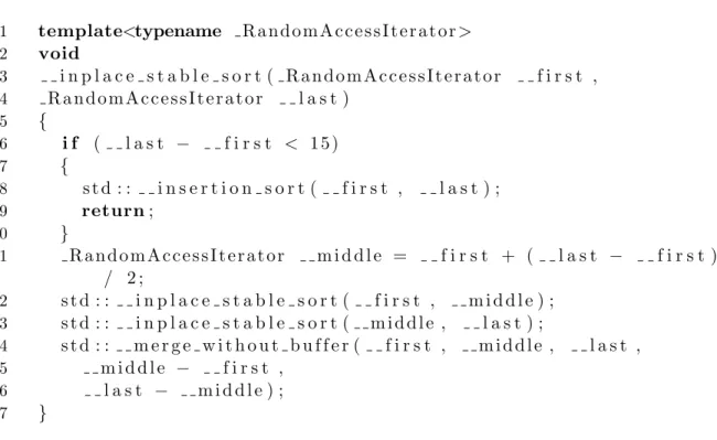
1-1 The STL std::sort routine. Insertion sort is used for inputs smaller than 15 elements, and merge sort is used for larger inputs. The 15-element cutoff is hard-coded into the library. From G++ 4.4 headers included with Ubuntu 10.10. . . 20

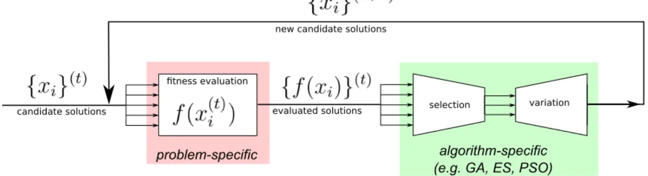
2-1 A functional diagram of an Evolutionary Algorithm. The algorithm evaluates candidate solutions using a problem-specific fitness function

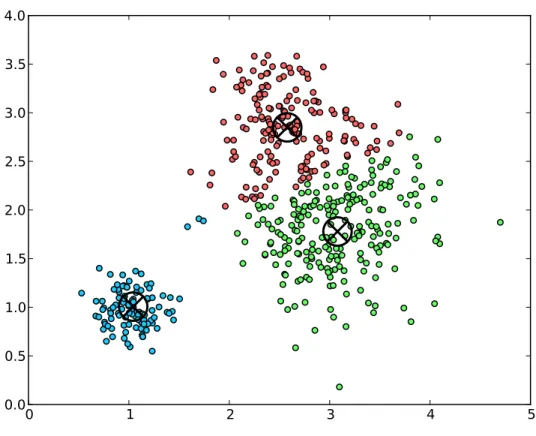
f, and produces new solutions using selection and variation operators, which differ by algorithm (adapted from http://groups.csail.mit. edu/EVO-DesignOpt/uploads/Site/evoopt.png). . . 27 2-2 An example run of thekmeansalgorithm on a set of 2-D points (Points),

with the number of clusters fixed at 3. The crosshairs mark cluster cen-ters (Centroids) and different point colors (Assignments) correspond to different clusters. . . 38 2-3 PetaBricks pseudocode for kmeans . . . 39 2-4 Dependency graph for kmeans example. The rules are the vertices

while each edge represents the dependencies of each rule. Each edge color corresponds to each named data dependence in the pseudocode. 40 2-5 A selector for a sample sorting algorithm where Cs = [150,106] and

As = [1,2,0]. The selector selects the InsertionSort algorithm for

input sizes in the range [0; 150),QuickSort for input sizes in the range [150,106_{) and RadixSort for [10}6_{, M AXIN T). BitonicSort was}

3-1 A sample genome form= 2, k= 2 and n= 4. Each gene stores either a cutoff cs,i, an algorithm αs,i or a tunable value ti. . . 52

3-2 Top level strategy of INCREA. . . 54

3-3 Pseudocode of function “fitter”. . . 56

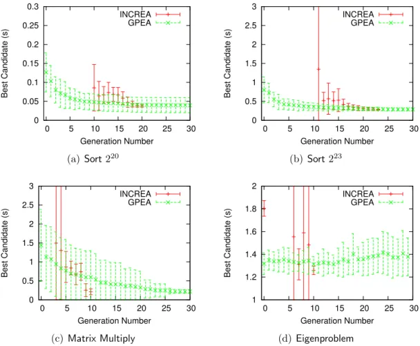
3-4 Execution time for target input size with best individual of generation. Mean and standard deviation (shown in error bars) with 30 runs. . . 59

3-5 Time out and population growth statistics of INCREA for 30 runs of

Sort on target input size 220. Error bars are mean plus and minus one standard deviation. . . 60

3-6 Representative runs of INCREA and GPEA on each benchmark. The left graphs plot the execution time (on the target input size) of the best solution after each generation. The right graph plots the number of fitness evaluations conducted at the end of each generation. All graphs use seconds of training time as the x-axis. . . 61

4-1 High level flow of the runtime system. The data on dotted lines may not be transmitted for the slower configuration, which can be terminated before completion. . . 69

4-2 Pseudocode of how requests are processed by the online learning system 74

4-3 The credit assigned to mutator µ is the area under the curve. Sec-tion 4.2.5 provides details. Reproduced from [29]. . . 79

4-4 Speedups (or slowdowns) of each benchmark as the load on a system changes. Note that the 50% load and 100% load speedups for Cluster-ing in (b), which were cut off due to the scale, are 4.0x and 3.9x. . . . 84

4-5 Representative graphs for varying system load showing throughput over time. Benchmark is LU Factorization on AMD48. . . 85

4-6 The scenario with frequent migration modeled by our architecture mi-gration experiments. We compare a fixed configuration (found with offline training on a different machine) to SiblingRivalry, to show how adapting to each architecture can improve throughput. We measure throughput only between the first and second migration, and include the cost of all learning in the throughput measurements. . . 87

4-7 Speedups (or slowdowns) of each benchmark after a migration between microarchitectures. “Normalized throughput” is the throughput over the first 10 minutes of execution of SiblingRivalry (including time to learn), divided by the throughput of the first 10 minutes of an offline tuned configuration using the entire system. . . 88

4-8 Representative graphs of throughput over time for fixed accuracy bench-marks after a migration between microarchitectures. . . 89

4-9 Representative graphs of throughput over time for variable-accuracy benchmarks after a migration between microarchitectures. “Target” is the accuracy target both the offline and online tuners are set to optimize for. . . 90

4-10 The effect of using an offline tuned configuration as a starting point for SiblingRivalry on the Sort benchmark. We compare starting from a random configuration (“w/o offline”) to configurations found through offline training on the same and a different architecture. . . 91

4-11 Average energy use per request for each benchmark after migrate Xeon8 to AMD48. . . 92

5-1 Best performing hyperparameters and associated score function values under the Static System and Dynamic System autotuning scenarios on Xeon8 and AMD48 architectures. . . 100

5-2 Metrics for benchmarkSort on theXeon8system evaluated with differ-ent values of hyperparameters. An asterisk ∗next to a number means that the difference from optimum is not statistically significant (p-value

≥0.05). . . 107

5-3 Metrics for benchmarkSort on theAMD48system evaluated with differ-ent values of hyperparameters. An asterisk ∗next to a number means that the difference from optimum is not statistically significant (p-value

≥0.05). . . 108

5-4 Metrics for benchmarkBin Packingon theXeon8system evaluated with different values of hyperparameters. An asterisk ∗ next to a number means that the difference from optimum is not statistically significant (p-value ≥0.05). . . 109

5-5 Metrics for benchmarkBin Packingon theAMD48system evaluated with different values of hyperparameters. An asterisk ∗ next to a number means that the difference from optimum is not statistically significant (p-value ≥0.05). . . 110

5-6 Metrics for benchmark Poisson on the Xeon8 system evaluated with different values of hyperparameters. An asterisk ∗ next to a number means that the difference from optimum is not statistically significant (p-value ≥0.05). . . 111

5-7 Metrics for benchmark Poisson on the AMD48 system evaluated with different values of hyperparameters. An asterisk ∗ next to a number means that the difference from optimum is not statistically significant (p-value ≥0.05). . . 112

5-8 Metrics for benchmark Image Compressionon the Xeon8 system evalu-ated with different values of hyperparameters. An asterisk ∗ next to a number means that the difference from optimum is not statistically significant (p-value ≥0.05). . . 113

5-9 Metrics for benchmark Image Compressionon the AMD48 system evalu-ated with different values of hyperparameters. An asterisk ∗ next to a number means that the difference from optimum is not statistically significant (p-value ≥0.05). . . 114

List of Tables

2.1 INCREA and SiblingRivalry compared to state-of-the-art autotuners from literature. . . 25

2.2 Listing of benchmarks and their properties. . . 44

3.1 INCREA and GPEA Parameter Settings. . . 57

3.2 Comparison of INCREA and GPEA in terms of mean time to conver-gence in seconds and in terms of execution time of the final configu-ration. Standard deviation is shown after the ± symbol. The final column is statistical significance determined by a t-test (lower is better). 58

3.3 Listing of the best genome of each generation for each autotuner for an example training run. The genomes are encoded as a list of algorithms (represented by letters), separated by the input sizes at which the resulting program will switch between them. The possible algorithms are: I = insertion-sort, Q = quick-sort, R = radix-sort, and Mx =

x-way merge-sort. Algorithms may have a p subscript, which means

they are run in parallel with a work stealing scheduler. For clarity, unreachable algorithms present in the genome are not shown. . . 63

3.4 Effective and ineffective mutations when INCREA solves Sort (target input size 220_{.) . . . . 63}

4.1 Specifications of the test systems used and the acronyms used to dif-ferentiate them in results. . . 82

5.1 Benchmark scores for the globally optimal values of hyperparameters normalized with respect to the best score for the given benchmark and scenario. The hyperparameters were C = 5, W = 5 for the Static System, and C = 5, W = 100 for the Dynamic System. Mean scores are 0.8832 and 0.8245 for the Static and Dynamic systems, respectively. 105

Chapter 1

Introduction

Despite the ever-increasing processing power of modern computers, high performance computation remains a commodity. A prime example are cloud services offered by companies such as Amazon, Google and Microsoft, where the user is billed depend-ing on the desired CPU resources. The use of such resources also affects energy consumption, which is important in systems ranging from embedded devices to large data centers [13]. For these reasons, users of computer software often demand efficient resource utilization, and a program that can perform the same work in less time, while also meeting some Quality of Service (QoS) guarantee, is usually considered better.

Unfortunately, optimizing software for optimal performance is a difficult feat and carries with it multiple caveats [3, 4]. While modern compilers attempt to take some of the optimization burden off the programmer, they are usually only successful at optimizing single algorithms and even then the range of possible optimizations is lim-ited [4]. In many applications, such as sorting, matrix multiplication and multigrid solvers significant performance boosts can be achieved by constructing hybrid algo-rithms, where the appropriate algorithm is chosen depending on the size of the input and hardware characteristics. However, the burden is on the programmer to incor-porate such hybrid algorithms, manually writing glue code and determining under what conditions the given algorithm should be invoked. Today’s compilers are unable to automate this process because of their reliance on traditional, low-level control structures such as loops and switches [3, 4].

What’s worse, it is often impossible to obtain a universal, “one-size-fits-all” solu-tion that achieves optimal performance on all hardware configurasolu-tions in all contexts. As such, software with hard-coded and often suboptimal algorithmic compositions is commonplace. An example can be found in the popular C++ Standard Template Library (STL) (Figure 1-1), whosesort routine uses insertion sort for inputs smaller than 15 elements and merge sort for inputs larger than 15 elements. Tests show that much larger cutoffs perform better on modern architectures [4].

1 template<typename R a n d o m A c c e s s I t e r a t o r> 2 void 3 i n p l a c e s t a b l e s o r t ( R a n d o m A c c e s s I t e r a t o r f i r s t , 4 R a n d o m A c c e s s I t e r a t o r l a s t ) 5 { 6 i f ( l a s t − f i r s t < 1 5 ) 7 { 8 s t d : : i n s e r t i o n s o r t ( f i r s t , l a s t ) ; 9 return; 10 } 11 R a n d o m A c c e s s I t e r a t o r m i d d l e = f i r s t + ( l a s t − f i r s t ) / 2 ; 12 s t d : : i n p l a c e s t a b l e s o r t ( f i r s t , m i d d l e ) ; 13 s t d : : i n p l a c e s t a b l e s o r t ( m i d d l e , l a s t ) ; 14 s t d : : m e r g e w i t h o u t b u f f e r ( f i r s t , m i d d l e , l a s t , 15 m i d d l e − f i r s t , 16 l a s t − m i d d l e ) ; 17 }

Figure 1-1: The STL std::sort routine. Insertion sort is used for inputs smaller than 15 elements, and merge sort is used for larger inputs. The 15-element cutoff is hard-coded into the library. From G++ 4.4 headers included with Ubuntu 10.10.

Unsurprisingly, automatic optimization of computer programs has been an active area of research. PetaBricks [4, 21, 7, 3, 5] is a is an implicitly parallel program-ming language for high performance computing which aims to solve the problems described above. It provides language constructs to naturally express algorithmic compositions through the concept of algorithmic choices. The programmer can sim-ply state what algorithms are applicable at the given point of the program, letting the compiler generate the necessary glue and decide how the algorithms should be com-posed. In addition to algorithmic choices, PetaBricks also allows the programmer to

define tunable parameters such as blocking sizes and the number of worker threads, whose optimal value is up to the compiler to select. The process of automatically determining algorithmic compositions and the values of tunables is called autotuning, and the autotuning program is called an autotuner. The autotuner’s goal is to find program configurations which maximize speed while meeting Quality of Service (QoS) guarantees.

1.1

Contributions

In this thesis we develop, evaluate and compare two PetaBricks autotuners: IN-CREA and SiblingRivalry. We provide experimental results for a large number of real-world benchmarks on a number of different architectures under different condi-tions.

INCREA makes the following contributions:

• It introduces a novel evolutionary algorithm for solving problems where evalu-ation is expensive and noisy.

• It can take advantage of shortcuts based on problem properties by reusing so-lutions to smaller problem instances when solving larger problems.

• It demonstrates that incremental solving works well on real-world problems.

In addition, SiblingRivalry makes the following contributions:

• To the best of our knowledge, the first general technique to apply evolutionary tuning algorithms to the problem of online autotuning of computer programs.

• A new model for online autotuning where the processor resources are divided and two candidate configurations compete against each other.

• A multi-objective, practical online evolutionary learning algorithm for high-dimensional, multi-modal, and non-linear configuration search spaces.

• A scalable learning algorithm for high-dimensional search spaces, such as those in our benchmark suite which average 97 search dimensions.

• Support for meeting dynamically changing time or accuracy targets which are in response to changing load or user requirements.

• Experimental results showing a geometric mean speedup of 1.8x when adapting to changes in microarchitectures and a 1.3x geometric mean speedup when adapting to moderate load on the system.

• Experimental results showing how, despite accomplishing more work, Siblin-gRivalry can actually reduce average power consumption by an average of 30% after a migration between microarchitectures.

1.2

Thesis Outline

The remainder of the thesis is organized as follows. Chapter 2 provides background on the PetaBricks language, the autotuning problem, evolutionary algorithms and the benchmarks used to evaluate autotuners. Chapter 3 presents and experimentally evaluates the offline autotuner INCREA. Chapter 4 describes the SiblingRivalry on-line autotuner and evaluates its performance on multiple architectures under different conditions. Chapter 5 performs an in-depth evaluation of SiblingRivalry’s sensitivity to hyperparameters. Finally, Chapter 6 draws conclusions.

Chapter 2

Background

2.1

Autotuning

For the purposes of this thesis, autotuning is a process of optimizing algorithmic choices and tunable parameters of a program in order to achieve the fastest possi-ble execution while meeting desired Quality of Service guarantees. We can classify different approaches to autotuning with respect to a number of independent criteria:

• generality: algorithm-specific vs. general-purpose

• hardware optimization capability: hardware-aware vs. hardware-oblivious

• number of objectives: single vs. multi-objective

• model dependence: model-based vs. model-free

• tuning process: online vs. offline

Generality of an autotuner specifies whether it can autotune arbitrary programs, or only a limited set of algorithms. For example, an algorithm-specific autotuner might be designed to optimize only the matrix multiplication algorithm in a specific math library. General-purpose autotuners can optimize any program written in a given language, and the programs that will be autotuned are generally not known when the autotuner is being implemented.

Hardware optimization capability of an autotuner defines whether it can adapt to different hardware configurations. Hardware-oblivious autotuners perform optimiza-tions that have a chance of improving performance independent of the machine that the tuned program runs on, but cannot take advantage of hardware-specific features such as hyperthreading, high memory bandwidth, or many others. Hardware-aware autotuners, on the other hand, can exploit both hardware-independent as well as hardware-specific optimizations.

Single-objective autotuners optimize only the running time of the program, at-tempting to produce the fastest possible executable, but cannot take advantage of possible beneficial trade-offs with other objectives inherent in the problem. For exam-ple, a single-objective autotuner cannot deliberately sacrifice accuracy to gain speed and vice-versa. Multi-objective autotuners, on the other hand, are built with such trade-offs in mind and can provide significant speedups by, for example, detecting when a program exceeds a user-defined accuracy target and decreasing the accuracy accordingly, saving execution time. While in principle multi-objective autotuners can deal with any number of objectives, in this thesis we limit ourselves to time and accuracy.

Model-based autotuners create a model of the program (and sometimes hardware) they tune and use it to their advantage. For example, a model-based autotuner might use the model to estimate the running time of a given program without actually run-ning it, saving computation. However, such models are at best only an approximation of reality and are designed with a number of assumptions in mind. Whenever those assumptions do not hold, the autotuner runs the risk of not being able to find the optimal configuration. Model-free autotuners, on the other hand, do not build models and instead optimize the tuned program directly. As a result, any execution intrica-cies, including those not predicted by the autotuner’s designers, can potentially be exploited.

Offline autotuners optimize their program once, usually at compile time, and re-use that static configuration throughout the lifetime of the program. Offline auto-tuning can be burdensome to the deployment of a program, since the auto-tuning process

Autotuner General-Purpose Hardware-Aware Multi-Objective Model-Free Online

INCREA Yes Yes No Yes No

SiblingRivalry Yes Yes Yes Yes Yes

ATLAS[53] No Yes No Yes No

FFTW[31] No Yes No No No

Green[13] Yes Yes Yes No Yes

PowerDial[35] Yes Yes Yes No Yes

Table 2.1: INCREA and SiblingRivalry compared to state-of-the-art autotuners from literature.

can take a long time and should be re-run whenever the program, microarchitecture, execution environment, or tool chain changes. Failure to re-autotune programs often leads to widespread use of sub-optimal algorithms. With the growth of cloud com-puting, where computations can run in environments with unknown load and migrate between different (possibly unknown) microarchitectures, the problems with offline autotuners become even more apparent. In contrast, online autotuners are always-on and can dynamically adapt to changes, automatically re-tuning a program when necessary.

Table 2.1 compares, along the above criteria, INCREA and SiblingRivalry against popular state-of-the-art autotuners described in literature.

2.2

Evolutionary Algorithms

The two autotuners presented in this thesis are based on Evolutionary Algorithms (EAs). Evolutionary Algorithms are stochastic global optimization methods that mimic Darwinian evolution, utilizing concepts such as inheritance, crossover, mu-tation and “survival of the fittest” [29]. EAs are a subset of a broader class of nature-inspired optimization algorithms which also include Artificial Neural Networks (ANNs), Particle Swarm Optimization (PSO), Ant Colony Optimization (ACO), and Simulated Annealing (SA), among others.

Within the domain of Evolutionary Algorithms, seminal work focused on tech-niques known as Genetic Algorithms (GAs), Evolution Strategies (ES), Evolutionary Programming (EP) and Genetic Programming (GP). Some other popular techniques

were introduced more recently, and include Differential Evolution (DE), and multi-objective evolutionary algorithms such as NSGA-II [26, 29, 28, 37]. Out of the above, GAs are described in more detail in Section 2.2.4.

Evolutionary Algorithms have been shown to be an effective optimization method for many problems where standard approaches failed. They can efficiently deal with vast search landscapes, landscapes in which the objective function is not differentiable and/or not well-specified (black box approaches), and can be robust in the face of a noisy objective function. The success of EAs in many difficult problem domains can be attributed to the large number of available techniques, and adjustable parameters in each that can be tailored to particular use cases [29].

Despite their differences, different EA methods follow a similar high-level approach (Figure 2-1), which can be summarized as follows:

1. A set of candidate solutions (the population) is generated, or reused from the previous generation(previous run of this loop).

2. The quality of candidate solutions is evaluated by a fitness function, which provides a numeric quality measure for each candidate (or multiple measures in the multi-objective case).

3. The fitness information from the previous step is used to select parentsolutions in a process termed selection. In general, the highest the fitness value of a candidate, the higher its chance of being selected.

4. Parent solutions are then subjected to variation operators such as crossover and mutation, which modify them slightly and thus generate new candidate solutions, theoffspring. These offspring, and sometimes certain parents, become the new population.

5. The process is repeated until some stop condition is reached, e.g. a candidate solution has been found which maximizes the fitness function or a specified number of generations has elapsed.

fitness evaluation

candidate solutions evaluated solutions new candidate solutions

problem-specific algorithm-specific

(e.g. GA, ES, PSO)

selection variation

Figure 2-1: A functional diagram of an Evolutionary Algorithm. The algorithm evaluates candidate solutions using a problem-specific fitness function f, and pro-duces new solutions using selection and variation operators, which differ by al-gorithm (adapted from http://groups.csail.mit.edu/EVO-DesignOpt/uploads/ Site/evoopt.png).

The variation operators are responsible for exploring the search space by introduc-ing random variation into the current population [29]. By applyintroduc-ing these operators only to the fittest individuals, we hope to explore only solutions which have the po-tential to be better than their parents. This is based on the locality assumption: small variation to a given candidate should produce small variations in its fitness. The selection component ensures that we do not accept solutions which are much worse than other candidate solutions in the population.

It is worth noting that Evolutionary Algorithms are most accurately thought of as high-level frameworks for solving problems, rather than complete and ready-to-use solutions. An EA expert will thus design variation operators, the fitness function and other components on a per-problem basis, and combine them into a functional algorithm using the outline given above.

The remainder of this section is organized as follows. Section 2.2.1 describes EA components that depend heavily on the problem and/or the particular EA technique being used to solve it. Section 2.2.2 covers components that depend on representation. Finally, section 2.2.3 describes universal EA components. This particular breakdown

is due to [29].

2.2.1

Problem-Specific Components

We now proceed to describe problem-specific components: fitness function and fitness evaluation, and representation. The exact form of these components depends heavily on the problem that they are used to solve.

Fitness Function and Fitness Evaluation

The fitness function, here denoted f, is responsible for providing a numeric quality measureqi for candidate solution xi:

f(xi) =qi, qi ∈Rd

where d is the number of objectives in the problem. For example, in the autotuning setting where d = 2, the fitness function returns a vector qi with two components:

runtime and accuracy. In the special case d = 1, we call f and the problem it representssingle-objective. Otherwise, whend ≥2, we call them multi-objective. The process of computing the fitness value for a given candidate solution is called fitness evaluation, or evaluation for short. Even though EAs are effective under a variety of fitness functions (and their geometric interpretation, fitness landscapes), an implicit requirement is that the fitness function be mostly continuous. If it is not, EAs tend to act like random search [29].

In some settings, such as program autotuning, the fitness function isstochasticor

noisy. This means that the values of f are samples from some underlying and often unknown probability distribution F. In such cases we assume that there exists one true fitness value equal to the mean of the underlying distribution, and the goal is to approximate it quickly and accurately.

Many EAs use a black-box approach to fitness evaluation, in which the values

f(xi) can be readily computed but little is known about f itself, and no closed form

time without invoking f, which can be problematic if fitness evaluations are costly. The cost and feasibility of fitness evaluation can be a major factor in the design of an evolutionary algorithm. Some approaches, such as Genetic Algorithms, often rely on a sizable population, whose evaluation at each generation might be prohibitive if

f is expensive to compute. In such cases, alternative methods such as Interactive Evolutionary Computation (IEC) are used [46].

Representation

A crucial issue in Evolutionary Computation is representation, or the low-level en-coding of candidate solutions [37]. Representation provides a bridge from the original problem context to the EA context where the actual optimization takes place [28, 29]. Objects in the original problem space are commonly referred to as phenotypes, while their encodings in the EA context are calledgenotypes, Formally, representation speci-fies a two-directional mapping from phenotypes to their corresponding genotypes [28]. The process of mapping phenotypes to genotypes is called encoding, while its inverse is referred to asdecoding. As an example, consider optimizing an integer-valued func-tion. The algorithm’s user might choose binary representation as the encoding, and hence the phenotype 42 would be encoded as 101010. Similarly, the phenotype 011111 would be decoded as 31.

While the distinction between phenotypes and genotypes might seem minor, it is important to understand that EA search happens in the genotype space [28]. The shape and characteristics of that space might be significantly different from those of the phenotype space. To that extent, a good representation encodes candidate solutions in a manner that makes the optimization easier by, for example, creating a smooth search landscape.

Two representations are of particular importance to the autotuners presented in this thesis:

• Integer representation: each candidate solution is encoded as a vector of inte-gers, where each integer is referred to as agene. A particular gene controls one or many (or none, in pathological cases) aspects of the individual’s phenotype.

• Tree representation: candidates are encoded as trees, which can represent e.g. decision trees for selecting the appropriate algorithm.

• Hybrid representation: candidate solutions are encoded as a combination of trees and integer vectors.

2.2.2

Representation-Dependent Components

Two EA components: initialization and variation operators, do not depend directly on the problem but on the representation [29]. We proceed to describe them in more detail.

Initialization

Initialization specifies how the initial (first) population gets chosen. In most appli-cations, it is relatively simple: the first population consists of individuals generated at random from some probability distribution [28, 29]. In others, a problem-specific heuristic is used. While in principle such heuristics could be used for any problem, their relative cost and benefits need to be evaluated on a per-problem basis [28].

Variation Operators

The role of variation operators is to explore the search space by creating new indi-viduals and thus introducing random variation into the population [28, 29]. We can classify variation operators into two categories: mutation and crossover, based on their arity. Arity in the context of variation operators specifies how many candidates an operator takes as inputs [28].

• Mutation is the name given to unary variation operators. It is applied to the genotype of one candidate solution, and outputs a slightly modified genotype commonly called a child or offspring. The modifications are usually stochastic [28]. The role of mutation varies by EC algorithm - in Evolutionary ming it is the only operator responsible for search, while in Genetic Program-ming it is often not used at all [28]. Regardless of the specifics, however, the

general role of mutation is to perform small steps in the search space and ensure that the space is connected, i.e. all the points are reachable given enough time. Connectedness ensures that a global optimum is theoretically obtainable [28].

• Crossoverorrecombination is the name given to variation operators of arity at least 2 [29]. Such operators produce offspring using information from at least two parent genotypes, and for that reason are often called sexual. The role of crossover is to combine different parts of parent genotypes into a new offspring solution, hoping that the offspring will retain and/or improve the good traits of its parents. Similarly to mutation, crossover is a stochastic process and choosing the parts to combine usually involves randomness. The role of recombination varies by EC algorithms - they are often the only variation operator in Genetic Programming, and an important one in Genetic Algorithms [42, 28]. In contrast, Evolutionary Programming does not use recombination at all [28].

2.2.3

General Components

Despite differences in fitness function, variation operators and representation, sur-prisingly many components are common to all EC algorithms. These components are outlined below.

Population

A population is a set of genotypes which represent candidate solutions currently under consideration. In a sense, population is the unit of evolution [28], because a standard EC algorithm operates by adapting and improving its population of solutions, rather than any single candidate solution. Given the parent population, an EC applies variation operators to selected individuals and thus produces the offspring population. There are two important metrics that describe populations: size and diversity. Size is simply the number of individuals within a population, and is usually constant. Choosing the right size is an important aspect of EC algorithm design, as it can affect search time and the algorithm’s robustness in noisy fitness settings [5, 18, 8].

Diversity, on the other hand, describes the amount of variation between candidate solutions. Common diversity metrics are the variance among fitness values, or the number of unique genotypes. Entropy is also sometimes used [28].

Parent Selection

Parent selection is the process of selecting parent solutions for use in mutation and recombination. The goal is to select only parents whose offspring have a high chance of improving their parents’ fitness. This is usually accomplished through some variant of fitness-proportionate selection, i.e. candidates with higher fitness values have a higher chance of being selected for reproduction. Low-quality candidates are selected more rarely, although in many applications they are selected sometimes in order to prevent the search from getting stuck in local optima [28]. Parent selection is generally randomized.

Survivor Selection Mechanism

Survivor selection is similar to parent selection in that its purpose is to distinguish candidates based on their quality. Unlike parent selection, however, it is applied

after offspring solutions have been generated. Since the population size is usually constant in EC, survivor selection is responsible for deciding which parents and which offspring are allowed into the next population (next generation). This process is usually deterministic: a fitness-biased EC might rank both parents and offspring by fitness and select only the first few, bounded by the preset population size. An age-biased EC, on the other hand, might select only from the offspring [28].

Termination Condition

Most EC algorithms have no guarantees about finding the optimum solution in some reasonable bounded time. As such, the algorithm’s user has to specify one or more heuristic termination conditions. Some common ones include [28]:

is known, and the search is terminated when it comes to within ± of that optimum.

• time limit: user-defined maximum running time has elapsed. Other related measures, such as CPU time, the number of generations or the number of fitness evaluations can be used as well.

• convergence: the search has converged, i.e. fitness improvement in the last few generations stayed below some small threshold.

• diversity loss: the population diversity drops below a predefined threshold.

In many cases, a combination of the above termination conditions is used. For example, an algorithm might be terminated either when it comes to within ± of optimum, or a time limit has passed, whichever comes first [28].

2.2.4

Genetic Algorithms

This section provides background on Genetic Algorithms, a variant of Evolutionary Algorithms implemented by the GPEA (Section 3.1) and thus most relevant to this thesis. Genetic Algorithms are the most widely know type of evolutionary algorithms, initially conceived by Holland as a means of studying adaptive behavior [28].

While there is some variation within genetic algorithms, some authors describe a “classical genetic algorithm” also known as the “simple GA” (SGA) [28]. The simple GA is single-objective (the fitness function returns a single number) and can be easily characterized using the component framework outlined in the previous section (2.2.3). The simple GA uses bit strings as its genotype representation, and maintains a population of candidates of constant size m [42, 28, 37]. A genotype in GAs is commonly referred to as the chromosome, and its length d is fixed. Recombination is achieved through 1-Point bit-wise crossover, where the value of a bit at the given position is replaced with the value of the corresponding bit in the other parent. The crossover operator is applied probabilistically with the crossover rate pc. That is,

probability pc. Otherwise, with probability 1−pc, offspring are created asexually by

copying the parents.

The most common mutation operator, known as uniform, randomly flips bits in the chromosome [42, 37]. More specifically, given a mutation probability pm, each bit

is independently flipped with probability pm. Thus for a chromosome of length d, an

expected number of pm×d bits are flipped.

Some GA variants, such as the GPEA presented in this thesis, use an integer representation with integers instead of single bits. The common variation operators in such a setting are defined analogously - mutation draws a random integer and crossover swaps corresponding integer values.

The simple GA uses fitness-proportional selection as the parent selection mecha-nism. That is, if the population consists of the candidates x1, x2, . . . , xm, the

proba-bility of a candidatexi becoming a parent is:

P r(xi is selected as parent) =

f(xi)

Pm

j=1f(xj)

Another common selection variant istournament selection. Instead of considering the entire population, tournament selection picks k individuals at random (with or without replacement), and adds the most fit one to the mating pool. This process is repeated until the mating pool has reached the desired size, usually equal to the population size m [28].

Survival selection in SGA is generational: the set of survivors is selected after the offspring have been generated. A common technique is age-based replacement, where the offspring completely replace the parents regardless of their fitness. This is the approach taken by the SGA. Another technique is fitness-based, where the age is ignored in favor of fitness. Many schemes that combine the two approaches exist. The one important to this thesis is elitism, introduced by Kenneth de Jong in 1975. Elitism works like age-based replacement, but the fittest member (or a fixed number of the fittest members) are always carried over to the next generation, regardless of their age [28, 42].

2.2.5

Multi-objective Algorithms

A special class of problems solved by Evolutionary Algorithms are multi-objective problems, i.e. problems where the fitness function f returns a vector with at least 2 components, each component corresponding to a different objective. While in prin-ciple multiple objectives could be reduced to a single objective through a weighted sum, in practice such sums may have no easy interpretation. More importantly, the designer might be interested exactly in how one objective might be traded off against another, a notion that a collapsed objective does not capture [37]. In such problems, the job of an EA is to optimize directly with respect to the multiple objectives [28, 37]. In the context of multi-objective optimization, an important notion is that of

Pareto Optimality. A solution is Pareto Optimal if none of its objectives can be improved without sacrificing at least one other objective [28, 37]. There can exist multiple Pareto Optimal solutions, corresponding to different objective trade-offs. We call the set of such solutions the Pareto optimal front, and individual solutions within that front non-dominated. Similarly, a solution is dominated if there exists another solution whose all objective values are at least as high, and at least one objective is strictly higher.

2.3

The PetaBricks Language

The PetaBricks language provides a framework for the programmer to describe mul-tiple ways of solving a problem while allowing the autotuner to determine which of those ways is best for the user’s situation [4]. It provides both algorithmic flexibil-ity (multiple algorithmic choices) as well as coarse-grained code generation flexibilflexibil-ity (synthesized outer control flow).

At the highest level, the programmer can specify a transform, which takes some number of inputs and produces some number of outputs. In this respect, the PetaBricks transform is like a function call in a procedural language. The major difference is that we allow the programmer to specify multiple pathways to convert the inputs to the outputs for each transform. Pathways are specified in a dataflow manner

us-ing a number of smaller buildus-ing blocks called rules, which encode both the data dependencies of the rule andC++-like code that converts the rule’s inputs to outputs. Dependencies are specified by naming the inputs and outputs of each rule, but unlike in a traditional dataflow programming model, more than one rule can be defined to output the same data. Thus, the input dependencies of a rule can be satisfied by the output of one or more rules. It is up to the PetaBricks compiler and autotuner to decide which rules to use to satisfy such dependencies by determining which are most computationally efficient for a given architecture and input. For example, on architectures with multiple processors, the autotuner may find that it is preferable to use rules that minimize the critical path of the transform, while on sequential architectures, rules with the lowest computational complexity may fair better. The following example will help to further illustrate the PetaBricks language.

2.3.1

Example PetaBricks Program: kmeans

Figure 2-3 presents an example PetaBricks program, kmeans, that implements the k-means clustering algorithm. The input to the algorithm is a set of n points

x1, x2, . . . , xn (Points) and the number of clusters k, k≤ n. The algorithm’s goal is

to find k cluster centers µ1, µ2, . . . , µk (Centroids) and partition of points between

the clusters S1, S2, . . . , Sk (Assignments) such that the following error function is

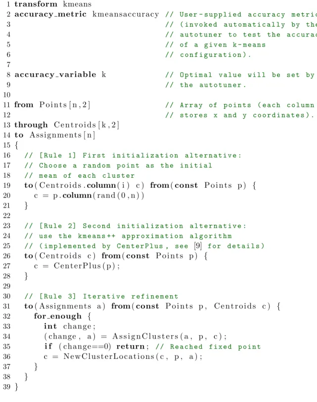
minimized [40]: arg min µ1,...,µk k X i=1 X xj∈Si ||xj −µj||2

Intuitively, the k-means algorithm tries to discover natural clusters in data, where the number k of clusters is specified beforehand by the user. An example run of k-means is shown in Figure 2-2.

The PetaBricks implementation of the k-means algorithm works as follows. It groups the inputPointsinto a number of clusters and writes each points cluster to the output Assignments. Internally the program uses the intermediate data Centroids to keep track of the current center of each cluster. The transform header declares each

of these data structures as its inputs (Points), outputs (Assignments), and interme-diate or “through” data structures (Centroids). The rules contained in the body of the transform define the various pathways to construct Assignments from Points. The transform can be depicted using the dependence graph shown in Figure 2-4, which indicates the dependencies of each of the three rules.

The first two rules specify different ways to initialize the Centroids data needed by the iterative solver in the third rule. Both of these rules require thePoints input data. The third rule specifies how to produce the outputAssignmentsusing both the input Points and intermediate Centroids. Note that since the third rule depends on the output of either the first or second rule, the third rule will not be executed until the intermediate data structure Centroids has been computed by one of the first two rules. Additionally, the first rule provides an example of how the autotuner can synthesize outer control flow. Instead of explicitly looping over every column of Centroids 2D array, the programmer can specify a computation that is done for each column of the output (using the column keyword). The order over which these columns are iterated, and the amount of parallelism to use, is then synthesized and tuned by the compiler and autotuner.

To summarize, when our transform is executed, the cluster centroids are initialized either by the first rule, which performs random initialization on a per-column basis with synthesized outer control flow, or the second rule, which calls the CenterPlus algorithm. CenterPlus implements the kmeans++ algorithm (not shown), details of which can be found in [9]. Once Centroids is generated, the iterative step in the third rule is called.

2.3.2

Variable Accuracy Algorithms

One of the key features of the PetaBricks programming language is support for vari-able accuracy algorithms, which can trade output accuracy for computational per-formance (and vice versa) depending on the needs of the user. Approximating ideal program outputs is a common technique used for solving computationally difficult problems, adhering to processing or timing constraints, or optimizing performance in

0

1

2

3

4

5

0.0

0.5

1.0

1.5

2.0

2.5

3.0

3.5

4.0

Figure 2-2: An example run of the kmeans algorithm on a set of 2-D points (Points), with the number of clusters fixed at 3. The crosshairs mark cluster cen-ters (Centroids) and different point colors (Assignments) correspond to different clusters.

1 transform kmeans 2 accuracy metric k m e a n s a c c u r a c y / / U s e r - s u p p l i e d a c c u r a c y m e t r i c 3 / / ( i n v o k e d a u t o m a t i c a l l y b y t h e 4 / / a u t o t u n e r t o t e s t t h e a c c u r a c y 5 / / o f a g i v e n k - m e a n s 6 / / c o n f i g u r a t i o n ) . 7 8 accuracy variable k / / O p t i m a l v a l u e w i l l b e s e t b y 9 / / t h e a u t o t u n e r . 10 11 from P o i n t s [ n , 2 ] / / A r r a y o f p o i n t s ( e a c h c o l u m n 12 / / s t o r e s x a n d y c o o r d i n a t e s ) . 13 through C e n t r o i d s [ k , 2 ] 14 to A s s i g n m e n t s [ n ] 15 { 16 / / [ R u l e 1 ] F i r s t i n i t i a l i z a t i o n a l t e r n a t i v e : 17 / / C h o o s e a r a n d o m p o i n t a s t h e i n i t i a l 18 / / m e a n o f e a c h c l u s t e r

19 to( C e n t r o i d s .column( i ) c ) from(const P o i n t s p ) {

20 c = p .column( rand ( 0 , n ) ) 21 } 22 23 / / [ R u l e 2 ] S e c o n d i n i t i a l i z a t i o n a l t e r n a t i v e : 24 / / u s e t h e k m e a n s + + a p p r o x i m a t i o n a l g o r i t h m 25 / / ( i m p l e m e n t e d b y C e n t e r P l u s , s e e [9] f o r d e t a i l s ) 26 to( C e n t r o i d s c ) from(const P o i n t s p ) { 27 c = C e n t e r P l u s ( p ) ; 28 } 29 30 / / [ R u l e 3 ] I t e r a t i v e r e f i n e m e n t 31 to( A s s i g n m e n t s a ) from(const P o i n t s p , C e n t r o i d s c ) { 32 for enough { 33 i n t change ; 34 ( change , a ) = A s s i g n C l u s t e r s ( a , p , c ) ; 35 i f ( change==0) return; / / R e a c h e d f i x e d p o i n t 36 c = N e w C l u s t e r L o c a t i o n s ( c , p , a ) ; 37 } 38 } 39 }

Figure 2-4: Dependency graph for kmeans example. The rules are the vertices while each edge represents the dependencies of each rule. Each edge color corresponds to each named data dependence in the pseudocode.

situations where perfect precision is not necessary. Algorithmic methods for produc-ing variable accuracy outputs include approximation algorithms, iterative methods, data resampling, and other heuristics. A detailed description of the variable accuracy features of PetaBricks is given in [3].

At a high level, PetaBricks extends the idea of algorithmic choice to include choices between different accuracies. Language extensions allow users to specify how accuracy should be measured for their transforms. The autotuner simultaneously optimizes for both performance and accuracy, producing a set of optimal algorithms that meet a range of accuracy levels. Users can specify whether they want output accuracy to be met statistically or guaranteed through the use of run-time accuracy checking.

The kmeansexample presented in Figure 2-3 is a variable accuracy algorithm. We briefly describe the variable accuracy features used in this example. Theaccuracy metric keyword on line 2 points to the user-defined transform,kmeansaccuracy, which com-putes the accuracy of a given input/output pair to kmeans. PetaBricks uses this transform during autotuning (and optionally at runtime) to test the accuracy of a given configuration of kmeans. The variable k (lines 8 and 13) controls the num-ber of clusters the algorithm generates by changing the size of the array Centroids. Sincek can have different optimal values for different input sizes and accuracy levels, declaring k an accuracy variable (line 8) instructs the autotuner to automatically find assignments of this variable during training to satisfy various levels of accuracy.

The for enoughloop on line 32 is a loop where the compiler can pick the number of iterations needed for each accuracy level and input size.

During training the autotuner will explore different assignments of k, algorithmic choices of how to initialize the Centroids, and iteration counts for the for enough loop to discover efficient algorithms for various levels of accuracy.

2.4

PetaBricks Autotuning

The autotuner must identify selectors that will determine which choice of an algorithm will be used during a program execution so that the program executes as fast as possible while meeting a user-defined QoS target. PetaBricks uses the accuracy of the program as the QoS, and hence that target is called theaccuracy target. Formally, a selectorsconsists of Cs = [cs,1, . . . , cs,m−1]∪As = [αs,1, . . . , αs,m] whereCs are the

ordered interval boundaries (cutoffs) associated with algorithmsAs. During program

execution the runtime function SELECT chooses an algorithm depending on the current input size by referencing the selector as follows:

SELECT(input, s) =αs,i s.t. cs,i> size(input)≥cs,i−1 where

cs,0=min(size(input)) andcs,m=max(size(input)).

The components of As are indices into a discrete set of applicable algorithms

available to s, which we denote Algorithmss. The maximum number of intervals

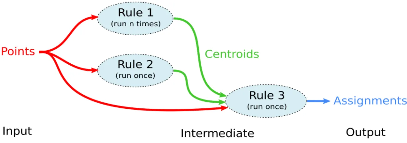
is fixed by the PetaBricks compiler. An example of a selector for a sample sorting algorithm is shown in Figure 2-5. In addition to algorithmic choices, the autotuner also tunes user-defined integer parameters (tunables) such as accuracy variables (see Section 2.3.1), blocking sizes, sequential/parallel cutoffs and the number of worker threads. Each tuned parameter is thus either an index into a small discrete set or an integer in some positive bounded range.

!_s,1 = 1 !_"#$ %& $'( )*+,-./01234 ( !"#5 % $(6 2-./0&"234 (7 RadixSort $7 InsertionSort 57 QuickSort 87 BitonicSort !_s,2 = 2 !_s,3 = 0 !"#$%&'()**+

Figure 2-5: A selector for a sample sorting algorithm where Cs = [150,106] and

As = [1,2,0]. The selector selects theInsertionSortalgorithm for input sizes in the

range [0; 150), QuickSort for input sizes in the range [150,106_{) and RadixSort for}

[106, M AXIN T). BitonicSort was suboptimal for all input ranges and is not used.

identify the vector of selectors S and vector of tunables T such that the following objective functionφ is maximized:

φ(S,T, P, H, n) =  



runtime(S,T, P, H, n)−1 if acc(S,T, P, H, n)≥acctarget

0 otherwise

In other words, the autotuner attempts to find a set of selectors S and tunables T which maximize program throughput (inverse of the running time) while meeting the user-specified target accuracy acctarget.

For each compiled program, the PetaBricks compiler produces a binary executable and a configuration file. The configuration file contains selector parameters As and

Csfor each algorithmic choice, as well as the vector of tunables T= [t1, . . . , tl]. Each

PetaBricks program contains a randomized generator of sample input data, and can be automatically benchmarked for any given input sizen without having to explicitly specify the input itself.

2.4.1

Properties of the Autotuning Problem

Three properties of autotuning influence the design of an autotuner. First, the cost of fitness evaluation depends heavily on the input data size used when testing the candidate solution. The autotuner does not necessarily have to use the target input size. For efficiency it could use smaller sizes to help it find a solution to the target size because is generally true that smaller input sizes are cheaper to test on than larger sizes, though exactly how much cheaper depends on the algorithm. For example, when tuning matrix multiply one would expect testing on a 1024×1024 matrix to be about 8 times more expensive than a 512×512 matrix because the underlying algorithm has O(n3_{) performance. While solutions on input sizes smaller than the}

target size sometimes are different from what they would be when they are evolved on the target input size, it can generally be expected that relative rankings are robust to relatively small changes in input size. This naturally points to “bottom-up” tuning methods that incrementally reuse smaller input size tests or seed them into the initial population for larger input sizes.

Second, in autotuning the fitness of a solution is measured in terms of how long it takes to run. Therefore the cost of fitness evaluation is dependent on the quality of a candidate algorithm. A highly tuned and optimized program will run more quickly than a randomly generated one and it will thus be fitter. This implies that fitness evaluations become cheaper as the overall fitness of the population improves.

Third, significant to autotuning well is recognizing the fact that fitness evaluation is noisy due to details of the parallel micro-architecture being run on and artifacts of concurrent activity in the operating system. The noise can come from many sources, including: caches and branch prediction; races between dependent threads to com-plete work; operating system artifacts such as scheduling, paging, and I/O; and, finally, other competing load on the system. This leads to a design conflict: an au-totuner can run fewer tests, risking incorrectly evaluating relative performance but finishing quickly, or it can run many tests, likely be more accurate but finish too slowly. An appropriate strategy is to run more tests on less expensive (i.e. smaller)

input sizes.

The INCREA exploits incremental structure and handles the noise exemplified in autotuning. We now proceed to describe a INCREA for autotuning.

2.5

Benchmarks

We show results from eight PetaBricks benchmarks to demonstrate the effectiveness of our online autotuning framework. Table 2.2 lists various attributes of each bench-mark, including which are variable and which are fixed accuracy. A brief description of our benchmarks follows.

Benchmark name Variable accuracy Search space dimensions

Sort No 33

Eigenproblem No 35

Matrix Multiply No 108

LU Factorization No 140

Bin Packing Yes 117

Clustering Yes 91

Helmholtz Yes 61

Image Compression Yes 163

Poisson Yes 64

Table 2.2: Listing of benchmarks and their properties.

2.5.1

Fixed Accuracy

Sort recursively sorts an array of integers utilizing various sorting algorithms (inser-tion, quick, merge, and radix).

Eigenproblemcomputes the eigenvalues and eigenvectors of a symmetric matrix using various numerical algorithms (divide and conquer, QR, and bisection).

Matrix Multiply performs multiplication of two dense matrices using various meth-ods including recursive decompositions and Strassen’s algorithm.

LU Factorizationperforms a factorization of a dense square matrix A=LU, com-monly used to solve linear systems.

2.5.2

Variable Accuracy

Bin Packing is an NP-hard problem that finds an assignment of items to unit sized bins such that the number of bins used is minimized, all bins are within capacity, and every item is assigned to a bin.

Clustering, or kmeans, is an NP-hard problem that divides a set of data into clus-ters based on similarity, which is a common technique for statistical data analysis in areas including machine learning, pattern recognition, image segmentation and computational biology.

Helmholtzsolves the 3D variable-coefficient Helmholtz equation, a partial differential equation that describes physical systems that vary through time and space, such as combustion and wave propagation.

Image Compression performs Singular Value Decomposition (SVD) on an m × n

matrix, which is a major component found in some image compression algorithms [52].

Poissonsolves the 2D Poisson’s equation, an elliptic partial differential equation that describes heat transfer, electrostatics, fluid dynamics, and various other engineering problems.

The benchmarks Sort and Matrix Multiply are described in more detail in [4]. The benchmarks Bin Packing, Clustering, Helmholtz Image Compression, and Poisson are described in more detail in [3]. Additionally an extensive study of the Poisson benchmark can be found in [21].

Chapter 3

Offline Autotuning

An off-the-shelf evolutionary algorithm (EA) does not typically take advantage of short cuts based on problem properties and this can sometimes make it impractical because it takes too long to run. A general short cut is to solve a small instance of the problem first then reuse the solution in a compositional manner to solve the large instance which is of interest. Usually solving a small instance is both simpler (because the search space is smaller) and and less expensive (because the evaluation cost is lower). Reusing a sub-solution or using it as a starting point makes finding a solution to a larger instance quicker. This short cut is particularly advantageous if solution evaluation cost starts high and grows proportionally with instance size. It becomes more advantageous if the evaluation result is noisy or highly variable which requires additional evaluation sampling.

This short cut is vulnerable to local optima: a small instance solution might become entrenched in the larger solution but not be part of the global optimum. Or, non-linear effects between variables of the smaller and larger instances may imply the small instance solution is not reusable. However, because EAs are stochastic and population-based they are able to avoid potential local optima arising from small instance solutions and address the potential non-linearity introduced by the newly active variables in the genome.

In this chapter, we describe the EA and associated offline autotuner called IN-CREA which incorporates into its search strategy the aforementioned short cut through

incremental solving. It solves increasingly larger problem instances by first activating only the variables in its genome relevant to the smallest instance, then extending the active portion of its genome and problem size whenever an instance is solved. It shrinks and grows its population size adaptively to populate a gene pool that focuses on high performing solutions in order to avoid risky, excessively expensive, explo-ration. It assumes that fitness evaluation is noisy and addresses the noise early when a lot of resampling is less expensive because smaller instances are being solved.

We will exemplify INCREA by solving the problem known as offline autotuning. Offline autotuning arises as a final task of program compilation in PetaBricks, and its goal is to select tunables and algorithmic choices for the program to make it run as fast as possible. Because a program can have varying size inputs, INCREA tunes the program for small input sizes before incrementing them up to the point of the maximum expected input sizes.

3.1

General-Purpose EA (GPEA)

We compare the performance of INCREA to that of an off-the shelf evolutionary algorithm that we call the General-Purpose EA or GPEA. We now proceed to describe GPEA in terms of the standard framework outlined in Section 2.2.

3.1.1

Representation

The GA represents configuration files as fixed-length chromosomes of length (2m+ 1)k+n, where k is the number of selectors, m the number of interval cutoffs within each selector and n the number of tunables defined for the PetaBricks program. We keep the number of intervals fixed across selectors, but retain the ability to have fewer effective ones by allowing intervals of length 0.

Each gene can assume any value in the range [0, M AXIN T), and encodes either a cutoff, an algorithm or a tunable value with a one-to-one correspondence (Figure 3-1). The respective decoding functions, φc, φα and φt are defined as follows:

cs,i=φc(c∗s,i) = $ Pi j=1c ∗ s,j Pm j=1c ∗ s,j ! M AXIN T % αs,j =φα(α∗s,j) = _α∗ s,j M AXIN T ||Algorithmss|| tj =φt(t∗j) =loj + _t∗ j M AXIN T (hij−loj)

The decoding functionsφα andφt scale the encoded genes linearly to within their

allowed ranges - [loj, hij) for tunables and [0,||Algorithmss||) for algorithms. The

cutoff decoder φc treats the encoded cutoffs as interval lengths, which it

normal-izes and sums to get the decoded cutoffs. This formulation of φc also ensures that

consecutive cutoffs are non-decreasing.

3.1.2

Initialization

Initial population consists of a fixed number of configuration files generated by ran-domizing all cutoff, algorithm and tunable values. The values are drawn from the same distributions which are used by the mutation operator.

3.1.3

Fitness Evaluation

We define the fitness of a genome as the inverse of the runtime. The runtime is obtained by timing the PetaBricks program for some input size n, with the decoded genome as its configuration file. The exact value of the input size is specified by the user.

Dealing with Noisy Fitness

Fitness variance is inherent in the autotuning process due to a varying system load. As a result, reported runtimes can be longer than the true ones, and cause inaccurate fitness values. To mitigate this problem, our GA can time genomes multiple times and use the minimum runtime. Since for large inputs evaluations can dominate the

GA’s runtime, we perform multiple timings only for small input sizes. The GPEA further deals with fitness noise by maintaining a large (100) population of candidate solutions. For a discussion on how population size can help in noisy settings, see [8, 18].

3.1.4

Variation Operators

The GA relies on single-gene crossover and mutation to generate successive popu-lations of configuration files. An offspring is generated by first crossing-over two parent configuration files, and then possibly mutating the result. The probability of a crossover is fixed at 1, i.e. all offspring are obtained through crossover, but the mutation probabilityP(mutation) is adjustable.

Crossover

Given two parents, the crossover operator chooses uniformly at random a single gene in both parents. If the gene encodes an algorithm αs,i, the offspring is then equal

to the first parent with αs,i substituted from the second. If, on the other hand, the

gene encodes a cutoff or a tunable, we either perform a similar substitution or choose a random value in between the two parents’ gene values, with a probability of the substitution vs. random choice equal P(substitution).

Mutation

After the crossover operator has been applied to two parents to produce an offspring, the offspring is mutated with probability P(mutation). The mutation operator se-lects, uniformly at random, a single gene from the offspring. The new value for that gene is then drawn from a different probability distribution depending on whether the gene encodes a cutoff, an algorithm or a tunable.

If the gene encodes an algorithm, the new value is drawn from a uniform proba-bility distribution 0− ||Algorithmss||. If it encodes a cutoff, the new value is a power

denotes the word size). However, if the gene is a tunable, then the distribution is chosen depending on the range of allowed values: uniform if the range is smaller than some constant R, i.e. hii−loi < R, and log-uniform otherwise.

3.1.5

Parent and Survivor Selection

Parents are selected using tournament selection with a fixed tournament size. Survivor selection is age-biased with elitism, where 95% of best offspring are carried over to the next generation, while the bottom 5% are replaced by the best candidates from the parent population.

3.1.6

Termination Condition

The GPEA terminates after a hard limit of 100 generations; there are no other ter-mination conditions.

3.2

Bottom-Up EA (INCREA)

3.3

Representation

The INCREA genome, see Figure 3-1, encodes a list of selectors and tunables as integers each in the range [0, M axV al) whereM axV al is equal to the cardinality of each algorithmic choice’s set for algorithms, and equal to M axInputSizefor cutoffs. Each tunable has a M axV al which is the cardinality of its value set or a bounded integer depending on what it represents.

In order to tune programs of different input sizes the genome represents a solution for maximum input size and throughout the run increases the “active” portion of it starting from the selectors and tunables relevant to the smallest input size. It has length (2m + 1)k +n, where k is the number of selectors, m the number of interval cutoffs within each selector and n the number of other tunables defined for the PetaBricks program. As the algorithm progresses the number of “active” cutoff