University of New Hampshire
University of New Hampshire Scholars' Repository
Master's Theses and Capstones Student Scholarship
Fall 2012
Object-based image analysis for forest-type
mapping in New Hampshire
Christina Czarnecki
University of New Hampshire, Durham
Follow this and additional works at:https://scholars.unh.edu/thesis
This Thesis is brought to you for free and open access by the Student Scholarship at University of New Hampshire Scholars' Repository. It has been accepted for inclusion in Master's Theses and Capstones by an authorized administrator of University of New Hampshire Scholars' Repository. For more information, please [email protected].
Recommended Citation
Czarnecki, Christina, "Object-based image analysis for forest-type mapping in New Hampshire" (2012).Master's Theses and Capstones. 741.
OBJECT-BASED IMAGE ANALYSIS FOR FOREST-TYPE MAPPING IN NEW HAMPSHIRE by Christina Czarnecki B.S., Philadelphia University, 2004 THESIS
Submitted to the University of New Hampshire in Partial Fulfillment of
the Requirements for the Degree of Masters of Science
in
Natural Resources
UMI Number: 1521564
All rights reserved
INFORMATION TO ALL USERS
The quality of this reproduction is dependent upon the quality of the copy submitted. In the unlikely event that the author did not send a complete manuscript
and there are missing pages, these will be noted. Also, if material had to be removed, a note will indicate the deletion.
UMI 1521564
Published by ProQuest LLC 2012. Copyright in the Dissertation held by the Author. Microform Edition © ProQuest LLC.
All rights reserved. This work is protected against unauthorized copying under Title 17, United States Code.
ProQuest LLC
789 East Eisenhower Parkway P.O. Box 1346
All rights reserved.
©2012
Tbis thesis has been examined and approved.
Thesi& Director, Dr. Russell G. Congalton, Professor of Remote Sensing and
Geographic Information Systems
Dr. Mark Ducey,
Br
oft Department of Natu and the EnvironmentResources
Earth Systems Research Center, University of New Hampshire
1
ACKNOWLEDGEMENTS
Funding was provided by a Mclntire-Stennis Research Assistantship (MS-33) (Congalton) offered by the University of New Hampshire Agriculture Experiment Station.
TABLE OF CONTENTS
ACKNOWLEDGEMENTS IV
LIST OF TABLES VII
LIST OF FIGURES VIII
ABSTRACT IX
INTRODUCTION 1
Objectives 4
LITERATURE REVIEW 5
Background 5
Land Cover Mapping: Pixels vs. Objects 8
Sampling Design and Data Collection 11
Data Preprocessing 16
Segmentation 18
Classification 22
Assessing Accuracy and Error 25
METHODS 31
Study Area 32
Ground Data Collection 33
Data Preprocessing 34
Segmentation 37
Training and Classification 38
Accuracy Assessment 41
RESULTS 43
Segmentation 43
Training and Classification 55
DISCUSSION AND SUMMARY 62
Collection of Reference Data 62
Classification Scheme 63 Accuracy Assessment 64 Other Remarks 66 Conclusion 69 LIST OF REFERENCES 70 APPENDICES 79 Appendix A 80 Appendix B 85 Appendix C 87
LIST OF TABLES
Table 1: Minimum and maximum spatial resolutions for selected optical
satellite sensors 11
Table 2: Description of fine-scale subclasses for forest cover classification
based on SAF definitions 14
Table 3: Spectral, spatial, and radiometric resolutions of IKONOS-2 sensor 32 Table 4: eCognition© class hierarchy used for classification 39
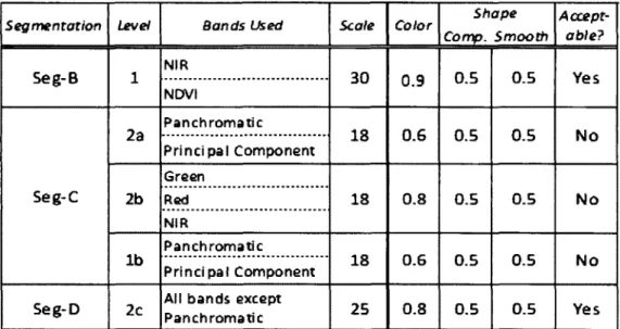
Table 5: Parameters used for segmentation 43
Table 6: MATRIX 1—error matrix applying the strictest rules for class membership—analyzed the 'best' class from both the reference
data and eCognition© 59
Table 7: MATRIX 2—error matrix analyzing the 'best' and 'acceptable' classes from the reference data, and the 'best' class from
eCognition© 60
Table 8: MATRIX 3—error matrix with the most relaxed rules—analyzed the 'best' and 'acceptable' classes from both the reference data
and eCognition© 61
LIST OF FIGURES
Figure 1: Example of a deterministic error matrix for a sample-based
classification 27
Figure 2: Example of an error matrix used for fuzzy accuracy assessment of a pixel-based classification; producer's, user's, and overall
accuracies are compared to a deterministic error matrix 29 Figure 3: Topographic overview of Pawtuckaway State Park and
surrounding study area 33
Figure 4: IKONOS false color image showing Pawtuckaway State Park
boundaries (south) and privately-owned land parcel (north) 36 Figure 5: Dialog box used to perform multi-resolution segmentation on
tier-4 classes 41
Figure 6: Level 1 -> Close-up of IKONOS panchromatic band under a transparent false color composite (above) and with seg-B
"vegetation-nonvegetation" results (yellow outline, below) 44
Figure 7: Level 2a -> Close-up of IKONOS panchromatic band (above) and
with seg-C "tree crown" results (yellow outline, below) 46 Figure 8: Level 2b -> Close-up of IKONOS panchromatic band (above) and
with seg-C "tree crown" results (yellow outline, below) 47 Figure 9: Level lb Close-up of IKONOS panchromatic band (above) and
with seg-C "tree crown" results (yellow outline, below) 48 Figure 10: Larger tree crowns are discernible in the lm2 panchromatic
band (above) but not in the 4m2 multispectral bands (below) 51 Figure 11: View of Pawtuckaway aerial images with seg-C (level 2a)
segments (below) and without segments (above) 52 Figure 12: Parameters used to create seg-D segmentation 53 Figure 13: Level 2c ->CIose-up of IKONOS panchromatic band (above)
and with seg-D results (yellow outline, below) 54 Figure 14: Nine dimensions used to separate vegetation from
non-vegetation 56
ABSTRACT
OBJECT-BASED IMAGE ANALYSIS FOR FOREST-TYPE MAPPING IN NEW HAMPSHIRE
By
Christina Czarnecki
University of New Hampshire, September 2012
The use of satellite imagery to classify New England forests is inherently complicated due to high species diversity and complex spatial distributions across a landscape. The use of imagery with high spatial resolutions to classify forests has become more commonplace as new satellite technology become available. Pixel-based methods of classification have been traditionally used to identify forest cover types. However, object-based image analysis (OBIA) has been shown to provide more accurate results. This study explored the ability of OBIA to classify forest stands in New Hampshire using two methods: by identifying stands within an IKONOS satellite image, and by identifying individual trees and building them into forest stands.
Forest stands were classified in the IKONOS image using OBIA. However, the spatial resolution was not high enough to distinguish individual tree crowns and therefore, individual trees could not be accurately identified to create forest stands. In addition, the accuracy of labeling forest stands using the OBIA approach was low. In the future, these results could be improved by using a modified classification approach and appropriate sampling scheme more reflective of object-based analysis.
INTRODUCTION
Remotely-sensed imagery from earth-observing satellites is commonly used in forest management to monitor or quantify land resources. Along with field-based measurements, satellite imagery is used extensively to monitor land cover
characteristics such as land cover types (forest, agriculture, urban, water, etc.) over a range of spatial and temporal scales (Dean and Smith, 2003; Carleer and Wolff, 2006; Ekercin, 2007; Hansen et al., 2008; Larranaga et al., 2011; Van Delm and Gulinck, 2011). By using remotely sensed imagery along with ground reference data, land managers are able to map their resources without having to make field
measurements at all of their managed areas. This technique of using imagery to map land cover increases efficiency and reduces the need to visit areas that are difficult or impossible to access. Maps derived from satellite imagery are known as thematic maps. Land cover maps are thematic maps that represent the ground, such as forest, pasture, water, or development. These land cover maps are useful in numerous natural resource applications to describe the spatial distribution and pattern of the land cover characteristics that they represent.
The ability to make accurate maps from remotely sensed data depends in part on the spatial resolution of the imagery. Spatial resolution is the surface area on the ground detected by the sensor, and is described as a pixel (Jensen, 2005). Pixel-based image classification has traditionally been the most common method to classify satellite imagery (Doraiswamy et al., 2004; Paul et al., 2004; Becker et al.,
2007; Roder et al.# 2008). Based on pre-determined rules, pixel-based classification categorizes all pixels in an image into a land cover category or theme that best describes them. The result is a thematic map that represents the different land cover types present on the image.
Over the last decade, the amount of high-resolution imagery available for analysis has greatly expanded sensor technology has progressed. Landsat TM, Landsat ETM+, and SPOT imagery, once considered to have high spatial resolutions, are now considered to have moderate resolutions at best because new even higher resolution data sensors have been introduced. Imagery from sensors like Quickbird and IKONOS is widely available and is being used for landscape analysis. Quickbird is a commercial satellite that offers 61cm panchromatic spatial resolution at nadir (the point on the ground directly below the sensor) and 2.4m multispectral spatial resolution at nadir. IKONOS (GeoEye, formally Space Imaging) is a commercial satellite that offers 80cm spatial resolution at nadir for the panchromatic band and 4m spatial resolution at nadir for the multispectral bands. Pixel-based classification is not as accurate when creating thematic maps from imagery with high spatial resolution as it is with moderate spatial resolution data (Blaschke and Strobl, 2001). This can be due to the effects of shadow or single ground objects fractured into many pixels (Townshend et al., 2000; Blaschke and Strobl, 2001).
An alternative to pixel-based classification is object-based image analysis (OBIA), a type of image processing and classification that has provided better results when using high resolution imagery. OBIA uses groups of pixels that represent a homogeneous area in a particular classification category. By averaging or grouping
like-pixels together, statistical separation can be achieved, thereby circumventing many of the problems faced when using pixel-based classifications with high-resolution imagery. Homogeneous landscapes are defined as land that is similar in composition or uniform in its patterns. Examples of similarly composed landscapes include single-species forests and large bodies of water. Uniform patterns include landscapes such as Christmas tree farms or crop fields, where trees or crops are not the only item on the landscape, but are dominant and appear equally spaced. In contrast, heterogeneous landscapes have no discernible pattern and are comprised of multiple features.
In general, more accurate land cover maps are created when classifying high resolution imagery with object-based techniques rather than pixel-based techniques (Descl£e et al., 2006; Yan et al., 2006; Cleve et al., 2008; Myint et al., 2011).
However, the ability of object-based classification methods to accurately identify individual trees in a forest, and also to identify individual trees by species, is an ongoing topic of research. In the past, New Hampshire forests have been classified using a system based on a classification scheme designed by the Society of American Foresters' (SAF). This classification scheme, first described by Eyre (1980), relies heavily on understory vegetation and ecological relationships to classify forest stands. This may not be conducive to creating accurate forest land cover maps based on satellite imagery. Therefore, the objectives of this study are:
Objectives
1. Evaluate OBIA as a means to identify individual tree crowns in a high-resolution forested image of New Hampshire, and merge these tree crowns to build forest stands
2. Evaluate OBIA as a means to create forest stand maps using the New Hampshire SAF classification system
CHAPTER I
LITERATURE REVIEW
The literature review is divided into six sections. The first section describes the fundamentals of satellite imagery and the basic types of image classifications. The second section compares two types of image classification techniques as they pertain to different types of satellite imagery. The third section describes the steps to gathering necessary field data to aid in image classification and creation of a classification protocol. Next, pre-processing of satellite imagery for classification is discussed. Then, the steps to OBIA are explained for creating thematic maps of forest cover types. Finally, an overview of the accuracy of thematic maps is explored.
PackgrQiind
Satellite-based sensors record radiance that reaches the sensor from the ground and atmosphere. Radiance is defined as the intensity of reflected light.
Sensors can be thought of as dividing the EM spectrum into one or more "bands" that measure radiance within a defined portion of the spectrum. A sensor can have several bands that measure radiance within different parts of the EM spectrum (Campbell and Wynne, 2011). The bands may be continuous or discrete, and wide or narrow. These characteristics refer to the spectral resolution of a satellite's sensor.
Areas on the ground are represented in a satellite image by pixels, which are organized into rows and columns. Each pixel's numerical value refers to the
radiance within that particular band. Low pixel values indicate high absorption of light, while high pixel values indicate high levels of light reflection. The ability of the sensor to distinguish slight differences in light intensity refers to its radiometric
resolution, which is measured in bits. Jensen (2005) defines radiometric resolution
as the sensitivity of the satellite sensor to detect differences in signal strength as it records the radiant flux reflected, emitted, or back-scattered from the terrain. Radiometric resolution is quantified as the levels of gray on an image. An 8-bit image will have up to 256 different pixel values, or 256 levels of gray. An 11-bit image that measures the same radiance as the 8-bit image will be able to measure up to 2,048 different pixel values, thereby capturing more detail or subtleties within the radiance than would the 8-bit image. Jensen (2005) likens radiometric
resolution to a ruler—if precision measurements are needed, a ruler with over 2,000 levels of gray is better than one with 256 levels of gray.
Individual pixels also represent a geographic area. The area of each pixel refers to the image's spatial resolution. The spatial resolution can be considered
coarse when it covers a large area (e.g., 1km2 or greater), or fine when it covers a small area (e.g., 60cm2).
Pixel-based image classification has traditionally been the most common method to classify satellite imagery (Dean and Smith, 2003; Jobin et al., 2008), where each pixel discretely categorized based on its spectral value. These
categories are set by the producer (the person performing the classification), and classification is facilitated using a supervised approach, an unsupervised approach, or a combination of the two (Jensen, 2005). In a supervised classification, the producer chooses training areas (defined homogeneous areas) that are
representative of a classification category. The spectral signatures of each training area are analyzed, and then all other pixels are classified based on those signatures. Supervised classification is best used when the categories of interest are easily defined and spectrally separable, the area of interest is relatively small, and the producer has in situ knowledge of the area. Unlike supervised classification, there are no training areas involved in unsupervised classification. Pixels in an image are separated into classes using a pre-defined number of categories and a confidence threshold. Once the pixels are divided into clusters, the producer then labels each class. Unsupervised classifications are best used when trying to classify relatively large areas on the ground, and for areas where there is little or no in situ knowledge (Jensen, 2005; Campbell and Wynne, 2011).
Recently, the high volumes of imagery available to land and resource managers—more specifically, the advent of multiple sources of readily available, high spatial resolution imagery—have made it necessary to take a different
approach to image classification. The large amount of data can become
overwhelming due to large file sizes, temporal abundance and variability, differing spatial and spectral scales, and the time-intensive methods used to interpret the data.
Land Cover Mapping: Pixels vs. Objects
The increase in spatial resolution means increased variability within areas that may have otherwise been defined as homogeneous. For example, on a spatially coarse image, a pixel might average the spectral reflectance of a group of oak trees. Another pixel might represent a wetland. As the spatial resolution becomes more refined, the group of trees becomes one tree, or only a part of tree. The wetland pixel is now several pixels that represent varying degrees of wetness within the wetland. A higher spatial resolution increases the spectral variability within the trees or wetland, and therefore can decrease the statistical separation between each pixel. These increases in spectral variability makes separability using pixel-based classification methods more difficult (Carleer et al., 2004).
The grouping of pixels in an image into objects, or segments, is called segmentation. Segmentation goes by several names in the literature, including segmentation, segment-based classification, object-based classification, region-based classification, and object-region-based image analysis (OBIA); objects can also be referred to as segments or polygons. Object-based image classification is an effective alternative to a pixel-based approach. A substantial difference between traditional pixel-based image classification and object-based classification is that
pixel-based classification does not use any spatial concepts (Blaschke and Strobl, 2001); classification is based on the spectral signature of a single pixel without consideration of other pixels around it. However, increases in spatial resolution increases the probability that pixels surrounding the pixel of interest are the same (Blaschke and Hay, 2001). As a result, the signal a pixel radiates as a representative of a particular class becomes contaminated by the signals of the pixels around it (Townshend et al., 2000). With an increase in spatial resolution comes a loss in statistical separability within the spectral data space, thereby reducing the accuracy of pixel-based classifications (Carleer et al., 2005).
The term "land cover" is used to describe different types of land. Common categories include forest, water, urban, and agriculture. This is different from "land use", which categorizes land based on its most common use. For example, while 'urban' describes a land cover type, 'residential', 'commercial', 'industrial', and 'transportation' are land use types. In the past, common types of imagery used to classify land cover included Landsat MSS, Landsat TM, MODIS, AVHRR, and others. The spatial resolutions of Landsat MSS and TM data are approximately 60m and 30m in the reflectance bands, respectively (Chander et al., 2009). MODIS products range from 250m - 1000m in spatial resolution depending on the product (LPDAAC, 2011). In traditional pixel-based classification, the spectral signal of each pixel across multiple bands of the electromagnetic spectrum is analyzed for
characteristics that separate it from different pixels on the same image. A single pixel represents a spectral aggregation of all land cover types within its boundaries. One or more land cover types would be represented within a single pixel.
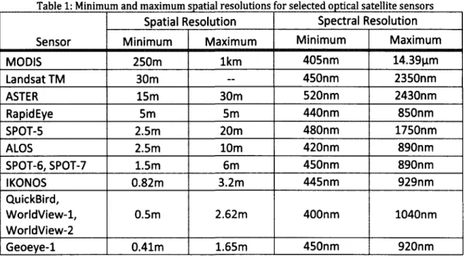
However, improvements in sensor technology allow for imagery with much higher spatial resolutions (Table 1). With this increase in spatial resolution comes a lower spectral resolution and a higher within-class spectral variability, thereby decreasing the statistical separability of spectral information into land cover classes. The biggest cause of increased internal variability within classes is pixels composed of shadow (Carleer et al., 2005). Another culprit that decreases separability is spatial autocorrelation, defined as the degree of dependency among observations in a geographic space; the signal of an individual pixel is highly influenced by the pixels around it (Townshend et al., 2000).
Object-based classification attempts to identify patterns in an image and use contextual information to group pixels into clusters that represent the same object. By grouping pixels into meaningful objects, spectral variability within a segment is minimized and differences between segments are maximized (Flanders et al., 2003). An object-based approach also reduces the effects of spatial autocorrelation. In general, high-resolution imagery is classified more accurately when using object-based classifications than pixel-object-based classifications (Townshend et al., 2000; Blaschke and Strobl, 2001; Coe et al., 2005).
Table 1: Minimum and maximum spatial resolutions for selected optical satellite sensors
Sensor
Spatial Resolution Spectral Resolution
Sensor Minimum Maximum Minimum Maximum
MODIS 250m 1km 405nm 14.39[im Landsat TM 30m — 450nm 2350nm ASTER 15m 30m 520nm 2430nm Rapid Eye 5m 5m 440nm 850nm SPOT-5 2.5m 20m 480nm 1750nm ALOS 2.5m 10m 420nm 890nm SPOT-6, SPOT-7 1.5m 6m 450nm 890nm IKONOS 0.82m 3.2m 445nm 929nm QuickBird, WorldView-1, WorldView-2 0.5m 2.62m 400nm 1040nm Geoeye-1 0.41m 1.65m 450nm 920nm
Sampling Design and Data Collection
A thematic map cannot be created without first devising a classification system. A good classification system starts with broad or generalized classes that allow for subdivisions into more specific classes; subdivision continues until a predefined, minimum-sized area is reached (Husch, 1971]. As these classes become more specific, the overlap in characteristics between classes lessens until mutually exclusive classes are developed. There are four main rules used when devising a classification scheme-that classes within the scheme be hierarchical in nature, devised of labels and rules, totally exhaustive, and mutually exclusive (Congalton and Green, 2009]. A hierarchical classification scheme is synonymous to
dichotomous key, where specific classes fall iteratively under more general descriptions. Each class should be clearly labeled and refer to its corresponding description. Also, each class description must adhere to a set of rules or definitions
that allow for a systematic and consistent classification. A totally exhaustive classification scheme ensures that every area on the map falls into a class, and that no area is left unclassified. Finally, a mutually exclusive set of classes ensures that each mapped area can only fall into one class. However, this final rule of sample exclusivity conflicts with the principles of fuzzy classifications, which is discussed in more detail in the next section.
For a forest classification system, a forest as a whole would be the most general class and be at the top of the class hierarchy. According to Husch (1971), there are three characteristics of a forest that can be used to devise a forest
classification system: size, site, and composition. A system based on size creates a class hierarchy based on such factors as tree height, basal area, or stand density (a forest stand is comprised of several trees grouped together). A system based on site would focus on qualities such as soil or terrain characteristics, or the general
purpose or use of the land. A system based on composition is the most widely used type of classification and focuses on species-specific characterizations (Husch, 1971).
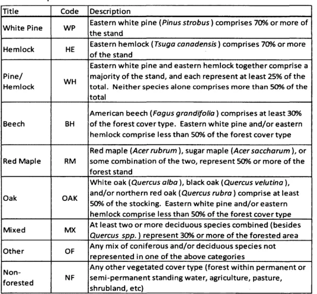
The composition-based classification system used for this study was based on rules and definitions set forth by the Society of American Foresters (SAF), which states that the dominant cover must be of trees, and must cover at least 25% of the area (see Table 2' for descriptions). Definitions of forest cover types are named after the predominant tree species, which is determined by basal area. The SAF defines a pure forest stand as stocked by 80% or more of a single species. A majority is comprised of a single species representing greater than 50% of a forest stand. A
plurality involves a single species that comprises the largest proportion in mixed
stands.
Forest classifications inherently include rules for categorizing forest species into stands and/or rules for sampling forests to determine stand types. Historically, sampling units have been categorized as either points or areal units. The term "point" is used to represent a correspondence between the resulting classification on the thematic map and its associated area on the earth. Areal units are defined by a spatial extent, such as a pixel, a polygon, or a unit of measurement (hectare, acre, square meter, etc.). It should be noted that although single pixels have been used as sampling units, they are often ineffective as such and instead should be used in clusters of pixels or another unit of measurement mentioned above (Congalton and Green, 1999,2009).
Stehman and Czaplewski (1998) released an overview of recommended sampling units using over thirty published works. Very few of these reviewed publications agree on a single "proper" sampling unit; however, it is agreed that a sampling unit must be optimized for its relevant application. The USDA Forest Service has used both points and areal units for its Forest Inventory and Analysis National Program (Birdsey and Schreuder, 1992). This program began in 1930 with systematic surveys of all forests by using areal extents. This technique was later changed to point-based sampling, where the points represent designated areas on the ground (ex. 20x20 plot). This was deemed more efficient and could be aided with the use of aerial photography. The USGS released a combined land use/ land cover classification scheme in an attempt to create a standardized system that could
be utilized by both private and government agencies (Anderson et al., 1976). The classification scheme uses only satellite imagery or aerial photography as its
reference for classification, and is hierarchical based on the spatial scale of imagery or photos used.
Table 2: Description of fine-scale subclasses for forest cover classification based on SAF definitions
Title Code Description
White Pine WP Eastern white pine (Pinus strobus) comprises 70% or more of the stand
Hemlock HE Eastern hemlock (Tsuga canadensis) comprises 70% or more of the stand
Pine/
Hemlock WH
Eastern white pine and eastern hemlock together comprise a majority of the stand, and each represent at least 25% of the total. Neither species alone comprises more than 50% of the total
Beech BH
American beech (Fagus grandifolia) comprises at least 30% of the forest cover type. Eastern white pine and/or eastern hemlock comprise less than 50% of the forest cover type
Red Maple RM
Red maple (Acer rubrum), sugar maple (Acer saccharum), or some combination of the two, represent 50% or more of the forest stand
Oak OAK
White oak (Quercus alba), black oak (Quercus velutina), and/or northern red oak (Quercus rubra) comprise at least 50% of the stocking. Eastern white pine and/or eastern hemlock comprise less than 50% of the forest cover type
Mixed MX At least two or more deciduous species combined (besides
Quercus spp.) represent 30% or more of the forested area
Other OF Any mix of coniferous and/or deciduous species not represented in one of the above categories
Non-forested NF
Any other vegetated cover type (forest within permanent or semi-permanent standing water, agriculture, pasture, shrubland, etc)
Data collection for image classification consists of two separate datasets: training datasets and reference datasets. The method used to collect data depends on several factors, including the minimum mapping unit (MMU, the minimum size for feature to be mapped), classification type [pixel or polygon), number of classes in the class hierarchy, and distribution of said classes on the image. Probability sampling is recommended for image classification because it takes into account the probability of a sampling unit being chosen for training or accuracy assessment, and thereby accounting for the percentage of that class that's present in the image (Congalton, 1991; Stehman and Czaplewski, 1998; Congalton and Green, 2009). There are several options for choosing a sampling scheme that include random, systematic, or stratified sampling schemes. Stratified random sampling is the most common sampling scheme used for image classification because it avoids spatial biases while ensuring that samples are collected for each of the classes, or strata, in the classification scheme (Stehman and Czaplewski, 1998; Congalton and Green, 1999; Radoux et al., 2011).
Reference samples and training samples should be chosen without replacement to ensure that the same sample isn't used for both classification training and accuracy assessment, thereby making accuracy assessment less efficient. Reference samples can be created by photo interpretation when possible and by field collection when photo interpretation is not possible. However, ground sample collection can be limited by such factors as time, money, and area
inaccessibility. Consequently, a minimum number of reference samples per class should be calculated ahead of time to ensure the statistical reliability of an accuracy
assessment. Collection of reference samples and training samples can be completed concurrently or separately. Congalton and Green (1999) recommend collecting 50 samples per class for areas totaling less than 1 million acres and with fewer than 12 classes as a "rule of thumb".
Data Preprocessing
Steps can be taken prior to image classification to enhance the satellite imagery. This preparation can yield new data layers for use with the original spectral bands, or can correct existing bands for errors due to geometry (errors in
pixel location) or atmospheric interference (spectral differences due to aerosol particles).
The creation of vegetation indices is a useful tool for extracting information in a pixel specific to vegetation health, phenology, or influences due to sun angle or sensor viewing angle. A vegetation index uses two or more image bands and
performs one or more mathematic operations the pixel's spectra. Vegetation indices can serve as a means to normalize data, differentiate vegetation from other surfaces that reflect light in the near-infrared, and emphasize particular spectral features that may otherwise be difficult to discern such as vegetation health. Some of the most common vegetation indices are a simple ratio (SR), the normalized difference vegetation index (NDVI), and the enhanced vegetation index (EVI) (Jensen, 2005),
SR = Pnlr (1) P red
where: SR = the ratio of reflected radiance from the red & infrared spectrum
pnlr = the reflected radiance within the near infrared spectrum Pred = the reflected radiance within the visible red spectrum
NDVI = Pred) (2)
(Pnir Pred)
where: NDVI = the normalized difference vegetation index pnir = the band within the near infrared spectrum Pred - the band within the visible red spectrum
EVI = G * - ^ (Pw'r * (1+ L) vPnir + Cl * Pred ~ ^2 * Pblue + *0
where: EVI = the enhanced vegetation index
pnir = the band within the near infrared spectrum
pred = the band within the visible red spectrum
G = gain coefficient Ci, C2 = aerosol coefficients
L = adjusts for effects from background
There are many other types of vegetation indices, but their utility is limited by the spectral extent and resolution of the sensor.
An important preprocessing step is to ensure that atmospheric interference due to clouds, water vapor, or aerosols are corrected. If left unaddressed, these interferences can limit spectral data interpretation. There are several different approaches to correcting an image for atmospheric interferences. One method, called Top-Of-Atmosphere (TOA) corrections, uses parameters obtained from the satellite's sensors (e.g. gain coefficients) as well as orbit data (e.g. time of year or sun angle) to correct pixel values (see 'Data Preprocessing', pg. 34) for correction.
Principal components analysis (PCA) can also be performed on multi-band imagery to reduce its dimensionality to only the most important information. Since the bands within a multispectral image are highly correlated, performing a PCA decorrelates the information by performing a transformation within the data's feature space and creating new "bands" that account for most of the variability in the original data. .
Segmentation
The human brain has the ability to recognize objects and perceive patterns, and naturally uses contextual information to understand what it's seeing; it
naturally segments what it's seeing into meaningful objects. Object-based classification attempts to replicate this process of recognition to overcome the limitations of pixel-based classification. Segmentation and classification of natural landscapes such as forested images must adhere to the basic principles of landscape ecology and attempt to capture the relationships between spatial patterns and related ecological processes (Farina, 2000; Turner et al., 2001; Burnett and
Blaschke, 2003). A landscape can be defined as a continuous spatial extent made up of a configuration of discrete patches in which ecological processes take place at different spatial and temporal scales (Farina, 2000). Scale is the spatial and temporal limit defined by the observer, and there are multiple scales within a landscape depending on perception or a given ecological process (Allen and Starr, 1988; Farina, 2000). The view that a landscape is neither a level of spatial
the study of landscape ecology, and on the whole has been abandoned in light of hierarchy theory (Allen and Starr, 1988; Wu, 1999; Farina, 2000; Blaschke and Lang, 2006; Farina, 2006). Hierarchy theory describes different spatio-temporal scales across a landscape.
Segmentation of a forested image requires breaking down a landscape (a continuous spatial extent) into discrete subsystems for the purposes of
classification. To achieve successful image classification, a segmentation algorithm must be chosen based on factors such as data types or intended use of the final product (Baatz and Schape, 2000; Philipp-Foliguet and Guigues, 2008). One such algorithm is the fractal net evolution approach (FNEA). FNEA is a multi-resolution or multi-scale approach, meaning that it operates on many different scales at once, and can be directly related to the way an ecologist might segment a landscape. Just as principles of landscape ecology and hierarchy theory use patches to divide a continuous landscape into discrete units, segments that are created from pixels in an image can be thought of as discrete patches. The size of the patch depends on the scale of interest. FNEA handles this ecological hierarchy by creating smaller
patches—smaller groups of pixels—and nesting them into bigger patches to create multiple levels. This makes FNEA an appropriate algorithm for image segmentation of a natural landscape. However, one problem when attempting to divide a
landscape continuum into discrete patches is the subjectivity of the divider; there are many ways that a continuous landscape can be divided (Burnett and Blaschke, 2003).
FNEA segments an image by identifying discontinuities between pixels (Blaschke and Strobl, 2001]. FNEA accounts for the representation of several scale domains in one image, and uses a region-merging technique starting with single-pixel objects. In numerous subsequent steps, smaller image objects composed of several pixels are merged into bigger objects. FNEA creates segments that follow a
homogeneity criterion, in which "the average heterogeneity of pixels [is] minimized.
Each pixel is weighted with the heterogeneity of the image object to which it belongs" (Baatz and Schape, 2000]. The goal is to increase between-object variability and decrease within-object variability (Flanders et al., 2003]. The collective result is multi-resolution segmentation, which captures objects on the image at multiple scales. This multi-scale technique is used to construct a hierarchical network of image objects. This network is topologically definite, meaning that all hierarchical levels are created by breaking segments down into sub-objects or grouping segments together into super-objects. Under-segmentation (multiple objects joined by one set of boundaries] and over-segmentation (a single object identified by multiple sets of boundaries] should be avoided (Carleer and Wolff, 2006].
When defining the parameters for image segmentation using FNEA, three homogeneity criteria are considered: scale, color, and shape. The scale parameter is an abstract and unitless number that controls the level of homogeneity in image objects created from segmentation. It represents a "degree of fitting", a threshold by which smaller segments are grouped into larger segments while still fulfilling the homogeneity criterion. In other words, smaller segments are grouped into larger
segments as long as the resulting segment maintains a particular threshold of homogeneity; once this threshold is met, the segment is no longer merged with other segments. Segmentations that use a low scale will have many smaller objects that are very homogeneous, while segmentations with higher scales will have larger image objects whose pixels are more heterogeneous. The homogeneity criteria values are chosen through trial-and-error until the chosen parameters result in a satisfactory segmentation.
The color parameter defines the amount of spectral information to be used in segmentation, and is the most important parameter for creating meaningful image objects. The color parameter determines the spectral bands to be used for
segmentation and how much influence they will have on segmentation. The shape
parameter is divided into two subcategories, compactness and smoothness. Color is
weighted with shape when creating image objects, meaning that more weight or importance placed on one parameter lessens the importance of the other parameter. Compactness and smoothness act together in the same way as do shape and color— when more weight is given to one, less weight must be given to the other.
Smoothness measures the ratio of the border length of an image object to the border
length of an adjacent image object. The smoothness parameter is useful when trying to extract very heterogeneous objects because it helps keep image object borders intact. The compactness parameter uses the ratio of border length to the square root of the number of pixels. This parameter is useful when separating compact objects from other image objects when there is a weak spectral contrast.
The standard deviation of the pixel values in a segment is variable depending on the homogeneity scale chosen (Kim et al., 2008). Finding optimal compactness and smoothness parameters depends on the size and type of object being extracted (Piatt and Rapoza, 2008). At least 10% of the criteria used for image segmentation must be given to both the color and shape parameter. However, because an image's spectral characteristics contain the best information for creating image objects, color should be given as much weight as possible while still using shape to achieve useful image objects.
ClassiflcatiQin
Once an image is divided into segments, a classification can be performed. The assumption that an object can only fall into a single category is not always accurate. This is only true if one is performing a deterministic classification (also known as crisp, hard, or binary classifications). Deterministic classifications work only when land cover classes are discrete in nature. By definition a landscape has a continuous and varying surface, and a fuzzy classification could prove a better and more accurate fit than a deterministic classification. With a deterministic
classification, misclassification can occur when dealing with pixels that prove difficult to sort into single land cover categories due to their within-class variance. Gaps in the tree canopy, shadows, and other components all comprise part of a land cover class but when included in a segment can confound a deterministic
classification (Foody, 1999). Fuzzy classifications allow thematic objects to have varying degrees of membership to one or more land cover categories. Foody (1999)
notes that the degree to which fiizziness is accommodated will be a function of the nature of data sets as well as practical constraints faced by the analyst.
A rule-based hierarchy is used to classify each segment. The rules at the top of a hierarchy trickle down and apply to all sub-classes below it. However, the placement of a segment into a fuzzy classification category is not binary—that is, it is not strictly a "yes" or "no" classification. Rather, a fuzzy-based classification gives each segment a percent chance of inclusion into each class. This technique of
classification is appropriate over a landscape, where land cover types are
continuous. Using forest classification as an example, fuzzy classification also takes into account error by the producer (e.g. selection of training samples), discrete thresholds set in the classification scheme (e.g. the percent tree cover that equates to forest), and the problem of intraclass variability within the segments (e.g. tree crown vs. tree shadow) (Foody, 1999).
Besides the spectral information present within a satellite image, other information within the image, such as an object's shape, context, or texture can be used to aid in classification. Information about an object's shape can include its size, length-to-width ratio, or perimeter. For example, an object representing a body of water could be classified as a lake or pond. If that object was more defined as a square or rectangle, it might instead be a reservoir; however, based on its small size, it might only be a swimming pool.
Also, the location of an object in an image within the context of other objects around it can help to classify it properly. For example, an object representing an area of grass may be classified as open pasture if it were surrounded by other
objects classified as vegetation. However, if it were surrounded by objects classified as urban features, then it is more likely that it is an urban or suburban park.
Texture refers to the spatial distribution of gray tones or the gray level variation of an image (Haralick et al., 1973; Ferro, 1998). One method of texture analysis is named the Gray Level Co-occurrence Matrix (GLCM), developed by R.M. Haralick (1973; 1979) to analyze the texture of image segments. First-order texture measures are non-spatial and use first-order statistics. Higher order texture
calculations are spatial because they use pixel neighbors in calculations; therefore, the placement of pixels within a moving window in relation to each other is
significant (Zhu and Yang, 1998). As such, more patterns present on a landscape may be discerned with higher order texture analysis than first order. In this respect, texture can be defined as a placement pattern within an image that is repeated and discernible, and it can be quantified in many ways, including mean, contrast, entropy, and directionality. Measurements of texture are functions of distance and angle. In the simplest terms, GLCM compares the gray level of a pixel (known as the reference pixel) to a pixel neighbor within a moving window, and each pixel within the window is analyzed with regard to its neighbor to detect a textural pattern. Gray values are compared in one or more directions, e.g. east (0°), northeast (45°), north (90°), or northwest (135°). The distance of the pixel neighbors to the
reference pixel can also vary; pixels may be directly next to each other or a defined distance away from each other.
Assessing Accuracy and Error
Once an image is classified into a thematic map, its accuracy should be determined before the map is used. There have been many studies that investigate accuracy assessment and recommend the best approach to estimating error, but the reality is that methods for assessing accuracy and error vary between studies
(Foody, 2002). Several factors can influence the accuracy of image classification. They include the MMU, sampling scheme, positional accuracy, and thematic
accuracy (Stehman and Czaplewski, 1998; Congalton and Green, 1999). MMU refers to the areal point, pixel(s), or polygon used to define reference data. The sampling scheme refers to the method used to collect reference data (discussed in the previous section 'Sampling Design and Data Collection'). These reference data are used as training parameters in classification as well as in accuracy assessment, also referred to by Stehman and Czaplewski (1998) as the evaluation protocol and labeling protocol respectively.
Positional accuracy refers to the actual coordinates of a pixel's location on the ground. It can be affected by image registration errors, terrain, or the angle of the sensor as it captured the image (Congalton and Green, 2009). Positional
accuracy can also be compromised when collecting GPS reference data points in the field. Factors such as tree cover, terrain, and atmospheric interference can affect the positional accuracy of collected data. Positional accuracy of GPS data can be
improved by using the Position Dilution of Precision (PDOP), a 3-D measure of the quality of GPS data (D'Eon and Delparte, 2005), to set a maximum allowable margin of error.
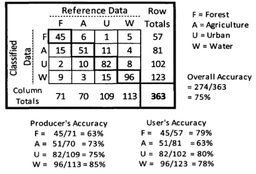
Thematic accuracy refers to the labeling of a classified image into categories. More specifically, it measures errors of commission (incorrect category label) and omission (not including data into the appropriate category). An error matrix, sometimes called a confusion matrix or contingency table, is a widely-adopted technique used to understand the accuracy of thematic maps produced from imagery (Congalton et al., 1983; Foody, 2002). An error matrix is a square array of numbers that computes producer's, user's, and overall accuracies of a thematic map (Figure 1).
Samples that are correctly classified reside in the error matrix on the major diagonal, and overall accuracy can be determined by dividing the total number of samples by the sum of the major diagonal. Producer's and user's accuracies were first introduced by Story and Congalton (1986) to more adequately display errors of omission and commission. The producer's accuracy is the probability that a selected area on the ground is classified correctly on the map; it resides in the matrix
columns. The user's accuracy is the probability that a classified sample on the map is the same as what is on the ground; it resides in the matrix rows. For example, in Figure 1, 71 reference samples were collected that represent the 'Forest' class; of those 71 samples, 45 were correctly classified. This means that of all the forested areas on the image, 63% of that area was classified correctly in the resulting
thematic map. On the thematic map, 57 samples were classified as 'Forest'; of those samples, 45 were correct. If a user were to take the thematic map in the field and attempt to locate all forested areas, the user would successfully locate forests 79%
of the time. By including producer's and user's accuracies in addition to the overall accuracy of an error matrix, one is able to pinpoint the classes causing confusion.
Reference Data Row
F A U W Totals j F 45 6 1 5 57 •- f A 4-5 M 15 51 11 4 81 co eg £ ° U 2 10 82 8 102 ° | W 9 3 15 96 123 Column Totals 71 70 109 113 363 F = Forest A = Agriculture U = Urban W = Water Overall Accuracy = 274/363 = 75% Producer's Accuracy F = 45/71 = 63% A = 51/70 =73% U = 82/109= 75% W = 96/113 = 85% User's Accuracy F = 45/57 = 79% A = 51/81 =63% U = 82/102 = 80% W = 96/123 =78%
Figure 1: Example of a deterministic error matrix for a sample-based classification
To quantify the randomness of an error matrix—e.g. is the classification of imagery into a thematic map better than random chance?—a Kappa coefficient can be generated (Cohen, 1960; Congalton et al., 1983). This is a "goodness of fit" test very similar to Pearson's Chi-Square test; it generates a KHAT statistic which measures the chance agreement vs. actual agreement of classes within an error matrix:
R = P o~ P c ( 4 )
1 ~~ Pc
where: R = statistical significance an error matrix po = the actual agreement between classes
pc = the chance agreement between classes
(Congalton et al., 1983)
KHAT values will range from 0 to 1, with 'zero' being completely chance agreement of classes, and 'one' indicating total statistical agreement of classes. A KHAT value greater than 0.8 represents strong agreement; a value between 0.4-0.8 represents moderate agreement; a value less than 0.4 represents poor agreement (Congalton and Green, 2009).
Traditionally, equally-sized sample units based on pixel size were used as ground reference data, and sample unit counts within classes were used in error matrices. However, there are two influences that should be considered when
designing an error matrix: this study makes use of segment-based classifications (as opposed to pixel-based), and uses fuzzy classifications (as opposed to deterministic classifications) and as such, modifications should be made to pixel-based
classification error matrices.
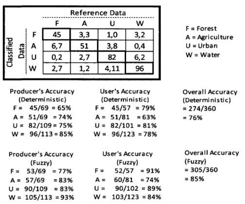
Deterministic classifications use a binary model when classifying samples, meaning that a sample either 'is' or 'isn't' classified correctly. However, with fuzzy classifications, samples may have varying degrees of membership to more than one classification category. This concept of "fuzziness" has also been explored relative to accuracy assessment (Congalton and Green, 2009). Instead of a yes/no
poor (Figure 2). The 'good' classification for a sample still resides in the major diagonal of the error matrix. However, both the 'acceptable' and 'poor'
classifications share the off-diagonal cells of the matrix, and are separated by a comma, respectively. When calculating the fuzzy producer's, user's, and overall accuracies, the 'acceptable' number in the off-diagonal cells (before the comma) are also included. Reference Data F A U W F 45 3,3 1,0 3,2 A 6,7 51 3,8 0,4 U 0,2 2,7 82 6,2 W 2,7 1,2 4,11 96 F = Forest A = Agriculture U =Urban W = Water
Producer's Accuracy User's Accuracy Overall Accuracy (Deterministic) (Deterministic) (Deterministic)
F = 45/69 = 65% F = 45/57 =79% = 274/360
A - 51/69 =74% A = 51/81 =63% = 76% U = 82/109 = 75% U = 82/101 = 81%
W = 96/113 = 85% W = 96/123 =78%
Producer's Accuracy User's Accuracy Overall Accuracy (Fuzzy) (Fuzzy) (Fuzzy)
F = 53/69 = 77% F = 52/57 = 91% = 305/360 A = 57/69 =83% A = 60/81 = 74% = 85% U = 90/109 = 83% U = 90/102 = 89%
W = 105/113 =93% W = 103/123 =84%
Figure 2: Example of an error matrix used for fuzzy accuracy assessment of a pixel-based classification; producer's, user's, and overall accuracies are compared to a deterministic error matrix
A Kappa analysis works well when all errors in an error matrix are of equal importance, as is the case with a deterministic classification (Congalton and Green, 2009). In the case of a fuzzy classification, a weighted Kappa can be used when errors vary in severity. For example, errors between vegetation strata are less
severe than if a vegetation sample is classified as water or an impervious surface. A weighted KHAT is defined as:
(5)
where: Rw = statistical significance of an error matrix
po = the weighted actual agreement between classes Pc = the weighted chance agreement between classes
(Congalton and Green, 1999)
One way to know if a classification's accuracy is better than random is to calculate a Z-score. This test is defined as:
At a 95% confidence value, if the absolute value of the Z-test is greater than 1.96, the result is better than random.
While both fuzzy classification and fuzzy accuracy assessment have been explored here, they are typically not combined due to the amount of uncertainty introduced into the final thematic map.
(6)
CHAPTER II
METHODS
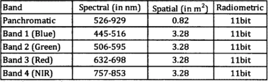
This study uses IKONOS satellite imagery to classify land cover via an object-based classification technique. IKONOS is a commercial satellite that has a revisit time of three to five days off-nadir, and approximately 144 days nadir. It is a sun-synchronous satellite that is pointable and able to be tasked, meaning that image acquisition over specific geographic areas can be prioritized. It has a spatial resolution as low as 80cm, and 4 multispectral bands (Table 3).
eCognition®, a proprietary object-based image processing software package developed by Definiens™ and now owned by Trimble™, was used to implement segmentation (FNEA algorithm) and classification of the IKONOS image and produce thematic maps of land cover information in the form of objects. Two thematic maps were produced with eCognition. The goal of each map was to differentiate tree species using IKONOS imagery. The first map depicts forests segmented into individual tree crowns. The second map depicts the forest divided into cover types as described by the SAF (Table 2).
Table 3: Spectral, spatial, and radiometric resolutions of IKONOS-2 sensor Band Spectral (in nm) Spatial (in m2) Radiometric
Panchromatic 526-929 0.82 libit Band 1 (Blue) 445-516 3.28 libit Band 2 (Green) 506-595 3.28 libit Band 3 (Red) 632-698 3.28 libit Band 4 (NIR) 757-853 3.28 libit
* resolution at nadir
Study Area
From 1750-1850, the New Hampshire landscape was characterized as mostly agriculture, with intense agriculture occurring after 1790 (Foster, 1992). Farm abandonment at the beginning of the industrial revolution allowed for the
reforestation of the state. As of 1997,84% of the state was forested (USFS, 2002). Remnants of this agricultural past remain, most obviously in the form of low stone walls that once divided pastures and farm boundaries (Foster, 1992; Allport and Howell, 1994; Foster and Aber, 2006). New Hampshire has an average growing season of approximately 151 days, receives an average of 120cm of rain each year, and an average of 150cm of snow each year (National Weather Service, 2011).
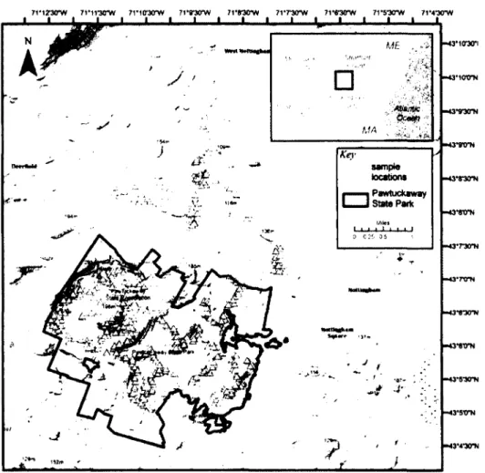
The study area (Figure 3) is comprised of two distinct parcels of land-Pawtuckaway State Park, a 4,000 acre state-managed park, and 4,600 acres of privately-owned land directly north of the park. The study area is located in the towns of Deerfield and Nottingham, both within Rockingham County, New
Hampshire. The 1KONOS scene is centered over the greater Mt. Pawtuckaway area. The altitude of the park ranges from 0m (sea level) to 303m (at Mt. Pawtuckaway). The park contains several recreation areas, including hiking trails, swimming, and camping, and is harvested infrequently for timber (Heath, 2008). The private land is
a sparsely settled residential zone, and covered mostly by forest, although several wetland areas exist. Approximately 25% of this private tract of land is actively harvested for timber (Lennartz, 2004).
71M2OTW 71M1,30,W 7riOOTW 7l*W(niV 71'8WW 71*7*30"W 71*6*30*W 71,M<rW TWaTW
riowi notrN •43*9WN •43WN rracrN -43 WN -43T30-N -43-7XTN -43*T30-N •"43*8 "0*N -43'5-3CTN -43*5TTN -43'4-30-N
Figure 3: Topographic overview of Pawtuckaway State Park and surrounding study area (Background map sources: USGS, FAO, NPS, EPA, ESRI, DeLorme, TANA)
Ground Data Collection
Sampling units were collected as 30m x 30m areas. Previous research (Pugh, 1997; Plourde, 2000; Lennartz, 2004; Heath, 2008) had established a composition-based classification scheme for this study area composition-based on the Society of American Foresters (SAF) description of the area (Eyre, 1980); a modified version of this
j—i—i—i— i l l ! Amm sample locations Pawtuckaway State Park
%
classification scheme was used for this study (Appendix A]. Samples were collected in forested areas. For this study, a forest is defined as having mature and/or
immature trees whose crowns touch or are within five meters of each other; forests are at least 1.25 acres in size, and are continuous across the landscape. Forest stands were classified based on the trees represented in the overstory. Trees that did not reach the upper canopy stratum, as judged using visual examination of relative crown positions, were not considered in the classification.
Ground reference sample units were collected during the summers of 2005 and 2006 using a quasi-random sampling technique designed to include as many different forest cover types as possible while staying restricted to roads, trails, and other areas that provided accessibility. Each sample unit represented the center of a 30mz sampling area. Once a plot center point was established, all trees that were within a 15m-radius and reached the top of the canopy were sampled. Ground reference points were collected using a Trimble TDC1 GPS unit. These points were manually corrected for positional accuracy using correction data supplied by a NH Department of Transportation base station in Concord, NH. An additional set of data points, collected in autumn 2007 and following the same collection rules, was also used to supplement existing ground reference points (Heath, 2008).
Data Preprocessing
A single IKONOS-2 scene with a swath width of 11.3km was used for this study. The scene was acquired by Space Imaging (now GeoEye) on September 5, 2001. The data were geometrically corrected prior to delivery and registered to the
New Hampshire State Plane (FIPS zone 2800, NAD 83 coordinate system). There is some cloud cover present on the image, but is less than 15% of the total image (Figure 4).
Although the image was orthorectified prior to delivery, it was not
atmospherically corrected. Aerosol particles in the air can cause light to refract and scatter, confounding image spectra interpretation. Common causes of atmospheric interference include clouds, haze, dust, and smog. Cloud cover is usually too dense to be corrected, and was therefore masked out of the image. To achieve the best possible image for classification, a Top-of-Atmosphere (TOA) correction algorithm was applied to the cloud-free image. This algorithm converts the raw DN (pixel digital number) into reflectance values, allowing index bands to be generated from the original bands for inclusion into segmentation and classification (Dial et al., 2001; Thenkabail, 2004; Chander et al., 2009). This is especially important with the inclusion of derivative bands into an image classification, such as Normalized
Difference Vegetation Index (NDVI) (Jensen, 2005; Hagen, 2010).
In a TOA correction, a conversion from raw pixel values to absolute radiance is performed first using the following equation (Chander et al., 2009):
DNj
La = CalCoefj ^
where: Lx = Spectral radiance at the sensor's aperture [(mW/cm2 sr)]
DNj = digital number of/h band [DN]
7ri330"W 71#1?30"W 71*11'30"W 71,10'3<rw 71 *9" 30 "W 7l'8"3ffW 7V7*30-W 7Vfl'3<rW I I I I I I I I I I I I I I I MS'*™ -43*r<rN -43'6-30*N »43'6'0*N »43'430*N
Figure 4: IKONOS false color image showing Pawtuckaway State Park boundaries (south) and privately-owned land parcel (north)
Next, absolute radiance of each pixel is converted to TOA reflectance using the following equation (Chander et al., 2009):
P p
I I * L x * dz
ESUNx * cos0s (8)
where: pv = Planetary reflectance [unitless]
n = 3.14159 [unitless]
Lx = Spectral radiance at the sensor's aperture [raW/ (cm2 sr)]
d = Distance from the sun to the earth [astronomical units]
ESUNx = Mean exoatmospheric solar irradiance [mW/ cm2] 0S = Solar zenith angle [degrees]
In an effort to spectrally separate vegetation features, three vegetation bands were generated in addition to the five original bands: a simple ratio (SR) band that compared the red and NIR spectra, a Normalized Difference Vegetation Index (NDVI), and an Enhanced Vegetation Index (EVI). Also, a principal components analysis (PCA) was performed on the four original multispectral bands in an effort to minimize the correlation of information between the bands (Carleer and Wolff, 2004). By performing a PCA, highly correlated information between bands are transformed into one or more component.
Segmentation
Segmentation is the crucial "first step" to classifying an image using OBIA because it lays the foundation for classified objects. Nine spectral layers were used in segmentation: the four multispectral bands of the IKONOS image, the
panchromatic band, a single principal component created from the original four multispectral bands, and the three vegetation indices. These bands together will be referred to as the pixel level of the image.
When defining the parameters for image segmentation using FNEA (see "Segmentation", pg. 19), the homogeneity criteria of scale, color, and shape are considered. The homogeneity criteria values are chosen through trial-and-error until visual inspection deems a satisfactory segmentation. The initial segmentation groups pixels together until the homogeneity criteria are met. This first
segmentation is the most important and will affect the outcome of all subsequent segmentations. Any further segmentation of the image will not begin with the pixel
layer but rather with this initial segmentation by further splitting the segments into sub-objects or grouping segments together into super-objects. Baatz et al. (2004) suggest that because of this, the initial segmentation should create objects as large as possible but as small as necessary. In order to keep track of the different levels of segmentation, each segmentation will be referred to with the 'seg' prefix.
From the pixel level of the image (referred to as seg-A), segmentation progressed over 4 stages. First, large generalized segments were created to separate all vegetation in the image from non-vegetation (seg-B). Second, these large vegetation segments were broken down into sub-objects that delineated individual tree crowns (seg-C). A final segmentation layer was created that grouped tree crowns into forest stands as defined by the SAF land cover classes (seg-D).
level: A -> B -> C -> D pixels -> vegetation -> crowns -> SAF
Objects in seg-B that were considered 'Non-Vegetation' were not further segmented in seg-C or seg-D.
Training and Classification
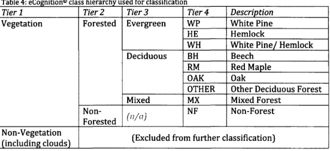
A class hierarchy was created to classify the image based on the modified SAF schema (Table 4). To differentiate between the different class hierarchies, the prefix 'tier' will be used. For all segmentations, two parent classes were initially created, 'Vegetation' and 'Non-Vegetation', to isolate all non-forest aspects of the image and remove their influences on species-specific forest classifications (tier-1 schema). Non-vegetated areas include open water, roads, buildings, and bare ground. The
'Vegetation' class was further divided into 'Forested' and 'Non-Forested' (tier-2 schema). Examples of non-forested categories present in the IKONOS image include grassy fields, some wetlands, and early successional growth. The seg-B
segmentation was classified using tiers 1&2 class hierarchy. Training areas for seg-B objects were chosen by visually interpreting the IKONOS image. Seg-C objects were classified to tree species, and seg-D objects were grouped into super-objects and classified according to the SAF-defined classes (tier-4 schema). Both seg-C and seg-D training data were collected via field sampling.
Table 4: eCognition® class hierarchy used for classification
Tier 1 Tier 2 Tier 3 Tier 4 Description
Vegetation Forested Evergreen WP White Pine Vegetation Forested Evergreen
HE Hemlock
Vegetation Forested Evergreen
WH White Pine/ Hemlock Vegetation Forested Deciduous BH Beech Vegetation Forested Deciduous RM Red Maple Vegetation Forested Deciduous OAK Oak Vegetation Forested Deciduous
OTHER Other Deciduous Forest Vegetation Forested
Mixed MX Mixed Forest
Vegetation
Non-Forested ( n / a )
NF Non-Forest Non-Vegetation
(including clouds) (Excluded from further classification)
Ground reference data were transferred from the GPS unit to an ArcGIS shapefile. Each point contained attributes of tree species found at the location (if it was a forested site) and other descriptive data. A total of 250 points out of 522 collected in the field were chosen to serve as training areas. These training samples were imported into eCognition® as a TTA (training and test area) mask. Once the
TTA mask was created, it was linked to the class hierarchy and could then be converted into training samples within eCognition©.
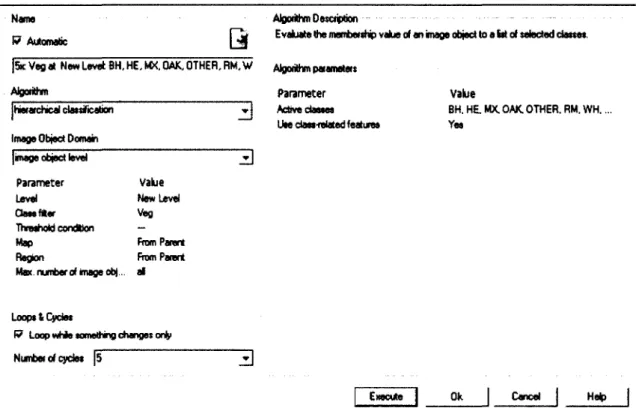
A divergence analysis was performed, called Feature Space Optimization (FSO) within eCognition®, to find the features that would best classify the segments (Appendix B). Divergence analysis is a statistical method used to select features that best separate two or more classes (Jensen, 2005). By optimizing the feature space, features were selected that best separate polygons into classes (Leduc, 2004; Durrieu et al., 2007). These features were then added to the classes as a nearest neighbor (NN) classifier. Nearest neighbor classifiers evaluated feature space overlap between samples and also managed overlaps during classification (Baatz et al., 2004). These overlaps in feature space were what allowed polygons to have fuzzy memberships to more than one class. eCognition© uses two types of nearest neighbor classifiers: standard NN and class-specific NN. By using the standard NN approach, features that were deemed optimal for class separation were applied to all classification categories equally; class-specific NN allows different optimal
features to be applied to different classification categories (Baatz et al., 2004; Leduc, 2004). For this study, the standard NN was modified.
Training areas were chosen so that samples were evenly distributed over the map. Polygon samples for seg-B objects included homogeneous areas such as grassy fields and closed canopy forest, as well as mixed samples such as polygons that grouped forest and open fields. The largest source of mixed samples was land cover edges and shadows created by tree canopy gaps. Segments that were classified as 'Non-Vegetation' in seg-B were not included in further classifications (Figure 5).