Perfect Graphs

University of Dayton

eCommons

Computer Science Faculty Publications

Department of Computer Science

2015

Perfect Graphs

Chinh T. Hoang

Wilfrid Laurier University

R. Sritharan

University of Dayton

Follow this and additional works at:

http://ecommons.udayton.edu/cps_fac_pub

Part of the

Graphics and Human Computer Interfaces Commons, and the

Other Computer

Sciences Commons

This Book Chapter is brought to you for free and open access by the Department of Computer Science at eCommons. It has been accepted for inclusion in Computer Science Faculty Publications by an authorized administrator of eCommons. For more information, please [email protected], [email protected].

eCommons Citation

Hoang, Chinh T. and Sritharan, R., "Perfect Graphs" (2015).Computer Science Faculty Publications. 87. http://ecommons.udayton.edu/cps_fac_pub/87

CHAPTER

28

Perfect Graphs

Chinh T.

Hoang*

R. Sritharan

t CONTENTS 28.1 28.2 28.3 28.4 28.5 28.6 28.7 28.8 28.9 28.10 Introd uction ... . Notation ... . Chordal Graphs ... . 28.3.1 Characterization ... . 28.3.2 Recognition ... . 28.3.3 Optimization ... . Comparability Graphs ... . 28.4.1 Characterization ... . 28.4.2 Recognition ... . 28.4.2.1 Transitive Orientation Using Modular Decomposition ... . 28.4.2.2 Modular Decomposition ... . 28.4.2.3 From the Modular Decomposition Tree to Transitive

Orientation ... . 28.4.2.4 How Quickly Can Comparability Graphs Be Recognized? .. 28.4.3 Optimization ... . Interval Graphs ... . 28.5.1 Characterization ... . 28.5.2 Recognition ... . 28.5.3 Optimization ... . Weakly Chordal Graphs ... . 28.6.1 Characterization ... . 28.6.2 Recognition ... . 28.6.3 Optimization ... . 28.6.4 Remarks ... . Perfectly Orderable Graphs ... . 28.7.1 Characterization ... . 28.7.2 Recognition ... . 28.7.3 Optimization ... . Perfectly Contractile Graphs ... . Recognition of Perfect Graphs ... . x-Bounded Graphs ... .

• Acknowledges support [rom NSERC of Canada.

t Acknowledges support from the National Security Agency, ForL Meade, Maryland.

708

710 710 710 712 715 715 715 718 720 720 721

722

725 726 727

728

728 729 729

731

732

733

733

735 735

738

741

742

744

J8 • Handbook of Graph Theory, Combinatorial Optimization, and Algorithms 28.1 INTRODUCTION

This chapter is a survey on perfect graphs with an algorithmic flavor. Our empha is i on important classes of perfect graphs for which there are fast and efficient recognition and optimization algorithms. The classes of gTaphs we discuss in this chapter are chordal, com-parability, interval, perfectly orderable, weakly chordal, perfectly contractile, and x-bound graphs. For each of these classes, when appropriate we discuss the complexity of the recog-nition algorithm and algorithms for finding a minimum coloring, and a largest clique in the graph and in its complement.

In the late 1950s, Berge [1 J started his investigation of graph. G with the following properties: (i) cx(G)

= 8(G),

that is the number of vertices in a largest stable set is equal to the smallest number of cliques that cover V(G) and (ii) w(G) = X(G), that is the number of vertices in a largest clique is equal to th smallest number of colors needed to color G. At about the same time, Shannon [2J in his study of the zero-error capacity of communication channels asked: (iii) what are the minimal graphs that do not satisfy (i)?, and (iv) what i the zero-enol' capacity of the chordless cycle on five vertices? In today's language, the graphs G all of whose induced subgraphs satisfy (ii) are called perfect.

In 1959, it was proved [3J that chordal graphs (graphs such that ev ry cycle of length at least four has a chord) satisfy (i), that is complements of chordal graphs are p rfect. In 1960. it was proved [1 J that chordal graphs are perfect. These two results led Berge to propo e two conjectures which after many years of work by the graph theory community were proyed to hold.

Theorem 28.1 (Perfect graph theorem)

rr

a graph is perfect, then so is its complement .

•

Theorem 28.2 (Strong perfect graph theorem) A graph is perfect if and only if it doe not contain an odd chord less cycle with at least five vertices, or the complement of uch a

cycle. •

Perfect graphs are prototypes of min-max characterizations in combinatorics and graph the-ory. The theory of perfect graphs can be used to prove well known theorems uch as the Dilworth's theorem on partially ordered sets [4J, or the Konig's theorem on edge coloring of bipartite graphs [5J. On the other hand, algorithmic considerations of perfect graphs have given rise to techniques such as clique cutset decomposition, and modular decompo ition. Question (iv) was answered completely in [6]; in the process of doing so, the so-called LOYI:\ z's theta function

e

were introduced. Theta function satisfies w( G) ::; 8( G) ~ X( G) for any graph G. Thus, a perfect graph G has w(G)

= 8(G) =

X(G). Subsequently, [7] gave a poly-nomial time algorithm based on the ellipsoid method to compute 8(G) for any graph G. A~ a consequence, a largest clique and an optimal coloring of a perfect graph can be found in polynomial time. Furthermore, the algorithm of [7] is robust in the ense of

[8]:

given th input graph G, it finds a largest clique and an optimal coloring, or says correctly that G is not perfect; [7J is also the first important paper in the now popular field of semidefinite programming (see [9]).

This paper is a survey on perfect graphs with an algorithmic flavor. Even though there are now polynomial time algorithms for recognizing a perfect graph and for finding an optimal coloring- and a largest clique- of such a graph, they are not considered fast or effici nt. Our emphasis is on important classes of perfect graphs for which there are fast and efficient recognition and optimization algorithms. The purpose of this survey is to discuss the e cla" es

Perfect Graphs • 7( of graphs, named below, together with the complexity of the recognition problem and the

optimization problems. The reader is referred to [10-12J for background on perfect graphs. Chordal graphs form a class of graphs among the most studied in graph theory. Besides being the impetus for the birth of perfect graphs, chordal gTaphs have been studied in contexts such as matrix computation and database design. Chordal graphs have given rise to well known search methods such as lexicographic breadth-first search and maximum cardinality search. We discuss chordal gTaphs in Section 28.3.

Comparability graphs (the graphs of partially order sets) are also among the earliest known classes of perfect graphs. The well-known Dilworth's theorem- stating that in a par-tially ordered set, the number of elements in a largest anti-chain is equal to the smallest number of chains that cover the set- is equivalent to the statement that complements of com-parability graphs are perfect. Early results of [13J and [14J imply polynomial time algorithms for comparability graph recognition. But despite much research, there is still no linear-time algorithm for the recognition problem. It turns out that recognizing comparability graphs is equivalent to testing for a triangle in a graph, via an O(n2

) time reduction. We discuss comparability graphs in Section 28.4.

Interval graphs are the intersection graphs of intervals on a line. Besides having obvious application in scheduling, interval graphs have interesting structural properties. For example, interval graphs are precisely the chordal graphs whose complements are comparability graphs. We discuss interval graphs is Section 28.5.

Weakly chordal graphs are graphs without chordless cycles with at least five vertices and their complements. This class of graphs generalizes chordal graphs in a natural way. For weakly chordal graphs, there are efficient, but not linear time, algorithms for the recognition and optimization problems. We discuss weakly chordal graphs in Section 28.6.

An order on the vertices of a graph is perfect if the greedy (sequential) coloring algo-rithm delivers an optimal coloring on the graph and on its induced subgraphs. A graph is perfectly orderable if it admits a perfect order. Chordal graphs and comparability graphs admit perfect orders. Complements of chordal graphs are also perfectly orderable. Recogniz-ing perfectly orderable graphs is NP-complete; however, there are many interesting classes of perfectly orderable graphs with polynomial time recognition algorithms. We discuss perfectly orderable graphs in Section 28.7.

An even-pair is a set of two nonadjacent vertices such that all chordless paths between them have an even number of edges. If a graph G has an even-pair, then by contracting this even-pair we obtain a graph G' satisfying w(G) = w(G') and X(G) = X(G'). Furthermore, if G is perfect, then so is G'. Perfectly contractile graphs are those graphs G such that, starting with any induced subgraph of G by repeatedly contracting even-pairs we obtain a clique. Weakly chordal graphs and perfectly orderable graphs are perfectly contractile. We discuss perfectly contractile graphs in Section 28.8.

Recently, a polynomial time algorithm for recognizing perfect graphs was given in [15J. We give a sketch of this algorithm in Section 28.9.

A gTaph G is x-bound if there is a function f such that X(G) :::; f(w(G)). Perfect graphs are x-bound. Identifying sufficient conditions for a graph to be x-bound is an interesting problem. It is proved in [16J that a graph is x-bound if it does not contain an even chOl'dless cycle. One many ask a similar question for odd cycles [17J: Is it true that a graph is x-bound if it does not contain an odd chordless cycle with at least five vertices? In Section 28.10, we discuss this question and related conjectures.

710 • Handbook of Graph Theory, Combinatorial Optimization, and Algorithms 28.2 NOTATION

For graph 0

=

(V, E) and x E V, Nc(x) is the neighborhood of x in G; we omit the subscript

o when the context

is clear. Let d(x) denote

IN(x)l.

For S ~ V, G[S] denotes the subgraph of 0 induced by S, and 0 - S denotes O[V - S]; for x E V, we use G - x for G - {x}. w (0) is the number of vertices in a largest clique in O. ex. ( G) is the number of vertices in a largest stable set in G. X (0) is the chromatic number of G.

e

(G) is the smallest number of cliques that cover the vertices of O. A clique is maximal if it is not a proper subset of another clique. For A, B ~ V such that OrAl and G[B] are connected, S ~ V is a separator for A and B provided A and B belong to different components of G - S. Further, S is a minimal separator for A and B if no proper subset of S is also a separator for A and B. We will al 0 call a set C of vertices a cutset if C is a separator for some sets A, B of V; C is a minimal

cutset if no proper subset of C is a cutset.

We use n to refer to

\VI

and m to refer to

lEI.

In a bipartite graph 0

= (X, Y, E), X and Yare the parts of the

partition of the vertex-set and E is the set of edges. A matching is a set of pairwise non-incident edges.

A set C of V is anti-connected if C spans a connected subgraph in the complement G of O. For a set X C V, a vertex v is X -complete if v is adjacent to every vertex of X. An edge is X-complete if both its endpoints are X-complete. A vertex v is X-null if v has no neighbor in X.

Ck denotes the chordless cycle with k vertices. A hole is the Ck with k ~ 4. An anti-hole is the complement of a hole. Pk denotes the chordless path with k vertices. K_t denotes the clique on t vertices. The K3 is sometimes called a triangle. The complement of a C₄ is denoted by 2K2 . The claw is the tree on four vertices with a vertex of degree 3.

For problems A and B, A ::; B via an f(m, n) time reduction means that an instance of problem A can be reduced to an instance of problem B using an algorithm with the worst case complexity of f(m, n); A

==

B via f(m, n) time reductions means that we have A

-<

B as well as B ::; A via f(m, n) time reductions.

Let 0 (n OC) be the complexity of the current best algorithm to multiply two n x n matrice . It is currently known that ex.

<

2.376 [18].

28.3 CHORDAL GRAPHS

Definition 28.1 A graph is chordal (or, triangulated) if it does not contain a chord less cycle with at least four vertices.

Chordal graphs can be used to model various combinatorial structures. For example, they are the intersection graphs of subtrees of a tree as we will see later. See [19] for application of chordal graphs to sparse matrix computations. Chordal graphs are among the earliest known classes of perfect gTaphs [3,20,21]. We will now discuss the combinatorial structure of chordal graphs.

28.3.1 Characterization

Definition 28.2 A vertex is simplicial if its neighborhood is a clique.

Theorem 28.3 [21] A graph 0 is chordal if and only if each of its induced subgraphs is a clique or contains two nonadjacent simplicial vertices. • To prove Theorem 28.3, we need the following two lemmas.

Perfect Graphs • 7

Proof Suppose C is a minimal cutset of G and AI, A2 are two distinct components of G - C. Further, suppose for x E C and y E C, xy tJ. E(G). As C is a minimal cutset of G, each of x, y has a neighbor in Ai, i

=

1,2. Let Pi, i

=

1,2, be a shortest path connecting x and y in G[Ai U CJ such that all the internal vertices of Pi lie in Ai· Then, G[V(PI ) U V(P2 )] is a

hole, a contradiction. •

Lemma 28.2 Let G be a graph with a clique cutset C. Consider the induced subgraphs _{GI , G2} with G = GIUG2 and GlnG2

=

C. Then, G is chordal if and onlyifGI ,G2 are both chordal. Proof If G is chordal, then as GI and G2 are induced subgraphs of a chordal graph, they themselves are chordal; this proves the only if part. For the if part, suppose each of GI , G₂ is chordal, but G has a hole L. Then, L must involve a vertex from each of GI - C, G_{2 -} C. Therefore, C contains a pair of nonadjacent vertices from L, contradicting C being

a clique. •

Proof of Theorem 28.3. The if part is easy: If G is a graph and x is a simplicial vertex of G, then G is chordal if and only if G - x is. Now, we prove the only if part by induction on the number of vertices. Let G be a chordal graph. We may assume G is connected, for otherwise by the induction hypothesis, each component of G is a clique or contains two nonadjacent simplicial vertices, and so G contains two nonadjacent simplicial vertices. Let C be a minimal cutset of G. By Lemma 28.1, C is a clique. Thus, G has two induced subgraphs GI, G2 with G = GI U G2 and GI

n

G2

=

C. By the induction hypothesis, each Gi has a simplicial vertex Vi E Gi - C (since C is a clique, it cannot contain two nonadjacent simplicial vertices). The vertices VI, v2 remain simplicial vertices of G, and they are nonadjacent. •

Definition 28.3 For a graph G and an ordering VI V2 ... Vn of its vertices, let G_i denote G[{ Vi, .. " vn}J· An ordering (J'

=

VI V2 ... Vn of vertices of G is a perfect elimination scheme (p. e. s.) for G if each Vi is simplicial in Gi ·

Theorem 28.4 [21,22J G is chordal if and only if G admits a perfect elimination scheme. Proof For any vertex v in a chordal graph G, G - V is also chordal; this together with

Theorem 28.3 prove the only if part. Since no hole has a simplicial vertex, the if part

follows. •

Corollary 28.1 A chordal graph G has at most n maximal cliques whose sizes sum up to at most m.

Proof By induction on the number of vertices of G. Let x be a simplicial vertex of G. Then,

{x}

UN

(x)

is the only maximal clique of G containing

x.

By the induction hypothesis, G -

x

has at most n -1 maximal cliques whose sizes sum up to at most m - d(x). Then, the result

follows. •

Definition 28.4 Let F be a family of nonempty sets. The intersection graph of F is the graph obtained by identifying each set of F with a vertex, and joining two vertices by an edge if and only if the two corresponding sets have a nonempty intersection.

Theorem 28.5 [23,24J A graph is chordal if and only if it is the intersection graph of subtrees of a tree.

2 • Handbook of Graph Theory, Combinatorial Optimization, and Algorithms

Proof. By induction on the number of vertices. We prove the if part first. Let G = (V. E) be a graph that is the intersection graph of a set 5 of subtrees of a tree T that is every vertex v of V is a subtree Tv of T, and two vertices 11, u E V are adjacent if and only if

Tv and Tu intersect. We may assume G is connected, for otherwise, we are done by vthe

induction hypothesis. By Lemma 28.2, and the induction hypothesis, we only need prove G is a clique, or contains a clique cutset. We may assume G is not a clique and let u v be two nonadjacent vertices of G. Then, Tu

n

Tv

=

0.

Let P

=

Xl,· .. , xp be the path in T with Xl E Tu, xp E Tv such that all interior vertices of P are not in Tu U Tv. Since T is a tree. P is unique; furthermore, all paths with one endpoint in Tu and the other endpoint in Tv

must contain all vertices of P. Thus, XIX2 is a cut-edge of T. Let S' be the set of all subtree of 5 that contains the edge XIX2. Then in G, the set C of vertices that corresponds to the subtrees of 5' forms a clique. We claim C is a cutset of G. In G, consider a path from uta t'; let the vertices of this path be u

=

tl, t2, ... , v

= tk·

Some subtree Tti must contain the edge Xl X 2 (because it is the cut-edge of T). Thus, the vertex that corresponds to Tti is in C. \Ye have established the if part.

Now, we prove the only if part. Let G

=

(V, E) be a chordal graph. We will prove that there is a tree T and a family 5 of subtrees of T such that (i) the vertices of T are the maximal cliques of G, and (ii) for each v E V, the set of maximal cliques of G containing v induces a subtree of T. The proof is by induction on the number of vertices. Suppa e that G is disconnected. Then, the induction hypothesis implies for each component C_i of G. there is a tree Ti satisfying (i) and (ii). Construct the tree T from the trees Ti by adding a new root vertex r and joining l' to the root of each Ti· It is easy to see that T satisfie (i)

and (ii). So, G is connected. We may assume G is not a clique, for otherwise we are ea ily done. Consider a simplicial vertex v of G. As v is simplicial in G, it is not a cut vertex of

G and therefore, G - v is connected. By the induction hypothesis, the graph G - 11 is the intersection graph of a set B of subtrees of a tree Ta satisfying (i) and (ii). Let J( be a maximal clique of G - v containing Ne(v) and let tk be the vertex of Ta that correspond to K. If K = Ne(v), then we simply add v to tK to get the tree T from Ta. Otherwi e. let K'

=

Ne(v) U {v}. Let T be the tree obtained from Ta by adding a new vertex tK' and the edge tktK" Let TK be the subtree formed by the single vertex tK', We can truct

5 as follows. Add TJ( to 5; for each tree Tv, E B, if Tu corresponds to a vertex in N G ( u), then add the tree Tu U {tJ(tKI}; otherwise, add Tu to 5. It is seen that (i) and (ii) hold for

T and 5. •

28.3.2 Recognition

Given G, an approach to testing whether G is chordal is: first generate an ordering IT of vertices of G that is guaranteed to be a perfect elimination scheme for G when G is chordal: then, verify whether 0" is indeed a perfect elimination scheme for G. The first linear-time

algorithm to generate a perfect elimination scheme of a chordal graph is given in [25]' it u e the lexicographic breadth-first search (LexBFS). We present the maximum cardinality earch algorithm for the same purpose.

The maximum cardinality search algorithm (MCS), introduced in [26], is used to con truct an ordering of vertices of a given graph; the ordering is constructed increm ntally right to left (if a comes before b in the order, then we consider a to be to the left of b). An arbitrary vertex is chosen to be the last in the ordering. In each remaining step, from the vertice' still not chosen (unlabeled vertices), one with the most neighbors among the alrcad cho en vertices (labeled vertices) is picked with the ties broken arbitrarily.

Algorithm 28.1 MCS

input: graph G

output: ordering (J"

=

VI V2 ... Vn of vertices of G

Vn f- an arbitrary vertex of G; for i f - n - 1 downto 1 do

Vi f - unlabeled vertex adjacent to the most in {Vi+I' .. "

vn

};

end for

Theorem 28.6 [26J Algorithm MCS can be implemented to run in O(m

+

n) time.

Perfect Graphs • 71 :

Proof We keep the array set [OJ ... set[n - 1] where set[j] is a doubly linked list of all the

unlabeled vertices that are adjacent to exactly j labeled vertices. Thus, initially every vertex

belongs to set[O]. For each vertex, we maintain the array index of the set it belongs to as

well as a pointer to the node containing it in the set[i] lists. Finally, we maintain last, the

largest index such that set[last] is nonempty. In the ith iteration of the algorithm, a vertex in

set[lastJ is taken to be Vi and Vi is deleted from set[last]. For every unlabeled neighbor w of Vi,

if w belongs to set[i], then we move w from set[i] to set[i + 1]. As each set is implemented as

a doubly linked list, a single addition or deletion can be done in constant time, and hence all

of the above operations can be done in O( d( Vi)) time. Finally, in order to update the value

of last, we increment last once and then we repeatedly decrement the value of last until set[lastJ is nonempty. As last is incremented at most n times and its value is never less than

-1, the overall time spent manipulating last is O(n) and we have the claimed complexity . •

Definition 28.5 For vertices x, V of graph G and an ordering (J of vertices of G, x

<()"

V

denotes that x precedes V in (J.

Lemma 28.3 [26J Let (J" be the output of algorithm MCS on chordal graph G. Then, G does

not have a chordless path P

=

(x

=

UO)U1 ... Uk-l(Uk

=

V) with k ~ 2 such that Ui

<()"

x,

1

5

i

5

k - 1, and x

<

()"

V·

Proof Suppose such a path existed; from all such chordless paths, pick P so that the position

of x in (J" is as much to the right as possible. Given the logic of the algorithm MCS, as

Uk-I

<cr

x

<cr

V, Uk-IV E E(G), and xV

(j.

E(G), there must exist a vertex z such that

x

<cr

z, xz E E(G), and Uk-IZ (j. E(G)). Let j be the largest index less than k-1 such that

UjZ E E(G); such a j exists as xz E E(G). Let pi be the path ZUj'" Uk-IV. As G is chordal

and pI has at least four vertices,

zv

(j.

E(G). Now, whether x

<

()"

z

<()"

V holds or x

<()"

V

<()"

Z

holds, existence of the chordless path pi violates the choice of P, a contradiction. •

Theorem 28.7 [26J If G is chordal, then the output (J"

=

VI V2 ... Vn produced by the algorithm

MOS is a perfect elimination scheme for G.

Proof Suppose not, and let i be the smallest such that Vi is not simplicial in Gi . Then, there

exist Vj and Vk such that Vi

<cr

Vj

<()"

Vk, ViVj E E(G), ViVk E E(G), and VjVk

(j.

E(G). Then,

714 • Handbook of Graph Theory, Combinatorial Optimization, and Algorithms

Algorithm 28.2 chordal-recognition

input: graph G

output: yes when G is chordal and no otherwise

Run algorithm MCS on G to get (J

=

VIV2'" Vn ;

if (J is a perfect elimination scheme for G then

output yes

else

output no

end if

Next, we discuss how to verify in linear time [25] whether (J

=

VI V2 ... Vn is a perfect

elimina-tion scheme for G. The key idea in [25] is that part of the work involved in checking whether

Vi is simplicial in Gi can be handed over to an appropriate vertex Vj such that Vi

<0"

Vj' In

particular, let Vj be the smallest neighbor of Vi such that Vi

<0"

Vj' Let

L(

Vi) = {Vk

I

Vj

<0"

Uk and ViVk E E( G)}. In other words, L( Vi) is the set of those neighbors of Vi that follow Vj in cr.

If Vj is simplicial in Gj and Vj is adjacent to every vertex in L(Vi), then Vi is simplicial in

G_{i . On th}e other hand, if either Vj is not simplicial in Gj or Vj is not adjacent to some vertex: in L(Vi) (making Vi not simplicial in Gi ), then (J is not a perfect elimination scheme for G.

Further, part of the work involved in checking whether Vj is simplicial in G_j can like wi e be

deferred to a later vertex.

In the following, the list bba(vk) is the list of vertices that Vk better be adjacent to; it i

the concatenation of the L(Vi) lists handed over to Vk by the Vi'S preceding it in cr.

Algorithm 28.3 pes-verification

input: graph G and ordering (J = VI V2 ... Vn of vertices of G

output: yes when (J is a p.e.s. for G and no otherwise

for i ~ I to n do

Initialize bba( Vi) to an empty list;

end for

for i ~ I to n - I do

if Vi is not adjacent to some vertex in bba( Vi) then

output no;

stop end if

Let Vj be the smallest neighbor of Vi such that Vi

<CT

Vj; L(Vi) ~ {Vk

I

Vj

<CT

Vk and ViVk E E(G)};

Append L( Vi) to bba( Vj)

end for

output yes

Theorem 28.8 [25] Algorithm pes-verification can be implemented to run in O(m+ n} time.

Proof. Assume that the array v[I]· .. v[n] stores (J. In order to ch ck whether Vi is adjacent

to every vertex in bba(vi): use a boolean array flag[I]··· flag[n] that is initialized in th first step of the entire algorithm. Now, mark the neighbors of Vi in the array flag. Then.

Perfect Graphs • 715

entry in flag is marked. Finally, unmark the neighbors of Vi in flag. Thus, this operation takes O(jbba(vi)j

+

d(vi)) time. As a vertex Vk hands over an L(Vk) list at most once, the total size of all bba lists is O( m + n) and the overall time spent on this operation is O( m

+

n). The rest of the operations can easily be implemented in O( m + n) time. •

28.3.3 Optimization

For a chordal graph, a largest clique and an optimal coloring can be found in linear time using the combined results in [25,27J. Even the weighted versions of these problems can be

solved efficiently. This will be discussed in the context of the more general class of perfectly

orderable graphs in Section 28.7.

The known optimization algorithms for chordal graphs use the clique cutset property. For

a general graph, there are polynomial time algorithms [28,29J to find a clique cutset if one

exists in the graph. [28,30J discuss optimization algorithm for classes of graphs, more general than chordal, using the clique cutset decomposition.

28.4 COMPARABILITY GRAPHS

Definition 28.6 A graph G

=

(V. E) is a comparability graph if there is a partially ordered set (P,

--<)

such that V = P and two vertices of G are adjacent if and only if the corresponding elements of P are comparable in the relation

-<.

Definition 28.7 An orientation of a graph is transitive if whenever a -t b, b -t c are arcs, a

-+

c is an arc.

An ordered graph (G,

--<)

corresponds to an orientation in a natural way: for vertices a, b, we

orient a

-+

b if a

-<

b. Now, we can redefine the notion of a comparability graph as follows. Definition 28.8 A graph is a comparability graph if it admits an orientation that is both acyclic and transitive.

28.4.1 Characterization

Several theorems on comparability graphs have become folklore. We start with a classical

theorem of [13J that as we will see later implies a polynomial time algorithm to recognize a comparability graph.

Theorem 28.9 [13J If a graph admits a transitive orientation, then it admits an acyclic and

transitive orientation. •

Definition 28.9 A subset M of vertices of a graph G = (V, E) is a module if any vertex outside of M is either adjacent to every vertex in M or adjacent to no vertex in M. Trivially,

{x} for any x E V, and V are modules. Module M is nontrivial if

jMj

2:

2

and MeV. To prove Theorem 28.9, we need the following.

Theorem 28.10 [13J If a graph admits a cyclic transitive orientation, then it contains a nontrivial module.

Proof Let G be a graph and let

G

be transitive orientation of G containing a directed cycle C. We may assume C is a shortest cycle and thus chordless. Since

G

is transitive, C has length three. We may assume G has at least four vertices, for otherwise the theorem is trivially

716 • Handbook of Graph Theory, Combinatorial Optimization, and Algorithms

outside C cannot have exactly one neighbor in C, for otherwise x and some two vertices in C

violate the transitivity of

C.

There must be a vertex v adjacent to exactly two vertices of C. for otherwise C is a nontrivial module of G. We may assume v is adjacent to b c. Let X be the set of vertices that are adjacent to b, c such that X is anti-connected,

a, v

EX, and X i

maximal with respect to this property. Since X is anti-connected, and a -+ b c -+ a, it follow

that every x E X has x -+ b, c

-+

x. We may assume X is not a module of G, for otherwi e

we are done. Thus, there is a vertex u r:J. X such that A = N('u)

n

X and B = X - A are

not empty. As X is anti-connected, there are vertices x E A, x' E B with XXi

rt.

E( G). Vertex

u must be adjacent to b, or

c,

for otherwise {u, x, b,

c}

violate the transitivity of

-a.

The maximality of X means u cannot be adjacent to both band c. We may assume ub E E(G). uc r:J. E(G). Now, {u,b,x'} or {u,b,c} violates the transitivity of

C.

•

Lemma 28.4 Let G be a graph with a nontrivial module X and x be a vertex in X. Let G₁ be the subgraph of G induced by (V (G) - X)

u

{x}, let G2 be the subgraph of G induced by X. Then G is a comparability graph if and only if both G1 and G 2 are.

Proof. We obviously need only to prove the if part. Assume both GI and G 2 admit acyclic

~ ~ -::t

transitive orientations G1 and G2 . An acyclic transitive orientation C; of G can be constructed as follows. Consider adjacent vertices a, b of G. If a -+ b is an arc in G1 or G 2, then let a -4 b be an arc of

C.

Otherwise, we may assume a E GI - x, bE X-x. If a

-+

x is an arc of G_{I .}

then let a

-+

b be an arc of

C,

else let b

-+

a be an arc of

G.

It is easy to verify that

-a

i

an acyclic transitive orientation. •

Lemma 28.4 implies the following.

Corollary 28.2 A minimally noncomparability graph cannot contain a nontrivial module . • Proof of Theorem 28.9. We prove by contradiction. Let G be a graph such that every tran-sitive orientation of G is cyclic. Therefore, G is not a comparability graph, and so G

con-tains an induced subgraph H that is minimally noncomparability. Therefore, every tran itiw'

orientation of H is cyclic. By Theorem 28.10, H contains a proper module, contradicting

Corollary 28.2. •

Definition 28.10 Let G = (V, E) be a graph. The corresponding knotting gmph is g'iven by K[G] = (VI(, EK) where VI( and EK are defined as follows. For each vertex v of G there are copies VI, V2, ... , Vi" in VI(, where iv is the number of components of G[N( v)]. For each edge vw of E, there is an edge ViWj in E K, where v is contained in the j th component of

G[N(w)]) and W is contained in the ith component of G[N(v)].

An illustration of the knotting relation is shown in Figure 28.1. It is easy to see that if G L

a comparability graph, then its knotting graph K (G) is bipartite. The converse is also true.

Perfect Graphs • 717

Theorem 28.11 [14J A graph is a comparability graph if and only if its knotting graph is

bipartite. •

A characterization of comparability gTaphs by forbidden induced subgraphs is given in [14]

(see [31J for an English translation of [14]).

Definition 28.11 A sequence IT

=

{YI W1Y2 ... Y2n+l W2n+1yd is an asteroid, more exactly a (2n

+

I)-asteroid, if the Yi are pairwise distinct vertices, each Wi is a path with endpoints Yi, Yi+l, and Yi has no neighbor in Wi+n (subscripts are taken modulo 2n + 1).

Theorem 28.12 [14J A graph G is a comparability graph if and only if its complement G

contains no asteroid. •

By characterizing all minimal asteroids, a list of all minimal non-comparability graphs can be found.

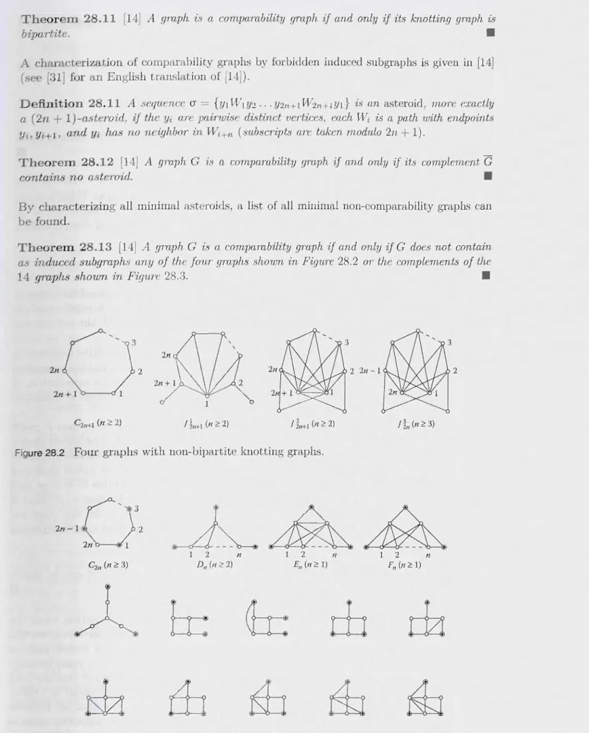
Theorem 28.13 [14J A graph G is a comparability graph if and only if G does not contain as induced subgraphs any of the four graphs shown in Figure 28.2 or the complements of the

14 graphs shown in Figure 28.3. •

2n 2 2 2n-l 2

0----<11

C2n+1 (n ~ 2) ;1,,+1 (n ~ 2) ;~n+l (n ~ 2)

Figure 28.2 Four graphs with non-bipartite knotting graphs.

0'

_{L A A}

2n-l 2 2n 1 1 2 n 1 2 n 1 2 n ~n (n ~ 3) Dn (n ~ 2) En (n ~ 1) En (n ~ 1)

~

tt

cb

ck

718 • Handbook of Graph Theory, Combinatorial Optimization, and Algorithms

The reader may verify that the graphs in Figure 28.2 have nonbipartite knotting graphs. and the graphs in Figure 28.3 contain a 3-asteroid.

Definition 28.12 Given a partial order (P, ~), a chain is a set of pairwise comparable

elements, an anti-chain is a set of pairwise incomparable elements.

A proof of the following well-known theorem is presented later.

Theorem 28.14 [4] In a partially ordered set (P,

-<),

the size of a largest anti-chain is equal

to the smallest n'umber of chains needed to cover all elements of P. • Let (P,

-<)

be a partial order, and let

G

be the transitive orientation of the comparability graph G of (P,

-<).

Because of transitivity, a directed path of

G

induces a clique. Thus a

chai~l

of P corresponds to a clique of G. And, an anti-chain of P corresponds to a stable set of G. Thus, Theorem 28.14 is equivalent to the statement that the complements of comparability

graphs are perfect. ~

28.4.2 Recognition

Consider the problem of determining whether a given graph G is a comparability graph. Equivalently, the problem asks if G can be oriented so that the resulting directed graph i acyclic and transitive. First, we consider an algorithm for the problem with the complexity of O(mn). Then, we discuss a more efficient algorithm.

Suppose G is a comparability graph, xy is an edge of G, and some transitive orientation

G

of G contains x ---+ y. Then, reversing the direction of every arc in

G

also yields a transitiYe orientation of G. Therefore, if we were to test whether G admits a transitive orientation. it

is enough to pick an arbitrary edge xy of G and determine whether there exists a tran itiYe orientation of G that contains x ---+ y.

Suppose xyz is a P3 of G. If a transitive orientation of G contains x -t y then it mu t contain z ---+ y also; in this situation, we say that x ---+ y forces z ---+ y. Now, the forced choic of z ---+ y might in turn force the orientation of some other edges. Th implication das of x ---+ y consists of all the arcs that are forced, in one or more steps, by the initial choice of x ---+ y. Clearly, for some edge uv, if the implication class of x ---+ y contains u -t v a well as v ---+ 'U, then G cannot be a comparability graph. Conversely, it can be shown [11] that if

the implication class of x ---+ y does not contain u ---+ v as well as v -t u, for any edge in"

then all the edges oriented thus far can be deleted from G, and the process can be repeat d on the remaining graph until it has no edges left.

Theorem 28.15 [11] Algorithm comparability-recognition-l is correct and it can be

imple-mented to run in O( mn) time. •

Algorithm comparability-recognition-1 produces an acyclic transitive orientation when th("

input graph is a comparability graph. Since the proof of its correctness is involved we will

not give it here. In this context, we note Theorem 28.9 already implies a simple polyno-mial time algorithm for recognizing comparability graphs: a graph G is a comparabilit~­ graph if and only if for each edge xy, the implication class of x -t y does not contain both

u ---+ v and v ---+ 'U for some vertices u, v. Since the number of P₃ of a graph is O(nm (each edge can be extended to at most n P3 ), it is not difficult to see that all impli a-tion classes of G can be enumerated in O(nm) time, and so this simple algorithm run~ in O(nm) time.

Algorithm 28.4 comparability-recognition-l

input: graph G

output: yes when G is a comparability graph and no otherwise

i = 1;

while G has edges left do

Pick edge xy and orient it x -r y;

Enumerate the implication class Di of x -r y;

if some u

-+

v and v -r u are in Di then

output no;

stop end if

Let Ei be the set of underlying edges of members of Di ;

G=G-Ei;

i = i

+

1

end while

output yes

Perfect Graphs • 719

Suppose we had an algorithm that can transitively orient a given comparability graph. Then,

we can combine that with an algorithm to verify whether a given orientation of a graph is

acyclic and transitive to obtain an algorithm to recognize comparability graphs. This is the

basis for the algorithm comparability-recognition-2.

Algorithm 28.5 comparability-recognition-2

input: graph G

output: yes when G is a comparability graph and no otherwise

Run on G an algorithm for transitively orienting a comparability graph to obtain the

directed graph

H;

if H is acyclic and transitive then

output yes else

output no end if

First, we consider the second step of the algorithm comparability-recognition-2, where it is

verified whether a given directed graph H is acyclic and transitive. The acyclicity of H can

be verified in linear time using standard search algorithms. Having done that, by considering

each P₃ of H, one can easily verify in O(nm) time whether H is transitive. A faster algorithm

can be derived using multiplication of Boolean matrices. The following is folklore.

Theorem 28.16 It can be verified in O(nC<) time whetheT a given directed acyclic graph G

i.'3 transitive.

Proof Let A be the adjacency matrix of G. Set each entry on the main diagonal of A to 1.

Then, G is transitive if and only if A = A2, where A2 is computed via multiplication of

Boolean matrices. •

In contrast to the verification step, a given comparability graph can be transitively oriented

720 • Handbook of Graph Theory, Combinatorial Optimization, and Algorithms

28.4.2.1 Transitive Orientation Using Modular Decomposition

The overall idea of the algorithm is to first decompose the given comparability graph using a technique called modular decomposition, store the result of the decomposition using a unique tree structure, and then orient the edges of the graph via a post order traver al of the decomposition tree. We note that modular decomposition of graphs in general has many other applications.

Suppose lVI is a nontrivial module in graph G

=

(V, E). Then, G can be decomposed into G₁

=

G[V - lVI U {x}] and G2

=

G[M], where x is any vertex in M. By Lemma 2 .4 G

is a comparability gl'aph if and only if G1 and G2 are. Therefore, the notion of modules i

directly relevant to the problems of recognizing comparability gl'aphs and finding a transitiYe orientation of a comparability graph. Lemma 28.4 shows when G is a comparability graph. it is easy to construct a transitive orientation of G from transitive orientations of G1 and G_{2 .} Therefore, when G is a comparability graph that has a nontrivial module one can find a transitive orientation of G by recursively solving the problem on G1 and G2 ; thus, the

problem essentially reduces to finding a transitive orientation of a comparability graph that has no nontrivial modules. In this case, the problem is solved using the fact [14] that such a

graph admits a unique transitive orientation (i.e., the transitive orientation and its rever~al

are the only possible ones). The notion of modular decomposition of a graph, described next.

is a systematic procedure to decompose a graph into modules and record the result as a

unique tree structure.

28.4.2.2 Modular Decomposition

The graph is decomposed recursively into subsets of vertices each of which is a module of the graph. The procedure stops when every subset has a single vertex. The result is represented as a tree.

Definition 28.13 A module which induces a disconnected subgraph in the graph is a parallel module. A mod1Lle which induces a disconnected subgraph in the complement of the graph i a series module. A module which induces a connected subgraph in the graph as well as in th complement of the graph is a neighborhood module.

If the current set Q of vertices induces a disconnected subgraph,

Q

is decomposed into it

components. A node labeled P (for parallel) is introduced, each component of Q is decom-posed recursively, and the roots of the resulting subtrees are made children of the P node. If

the complement of the subgraph induced by current set Q is disconnected,

Q

is decompo...,ed

into the components of the complement. A node labeled 5 (for series) is introduced, ea h component of the complement of Q is decomposed recursively, and the roots of the re ulting

subtrees are made children of the

5

node. Finally, if the subgraph induced by the current set Q of vertices and its complement are connected, then

Q

is decomposed into its ma..'cim.al proper submodules (a proper submodule lVI of

Q

is maximal if there does not exist modul

lVI' of

Q

such that lVI

c

lVI'

c

Q);

it is known [14] that in this case, each vertex of Q

belong.:-to a unique maximal proper submodule of

Q.

A node labeled N (for neighborhood) is i ntro-duced, each maximal proper submodule of

Q

is decomposed recursively, and the roots of the resulting subtrees are made children of the N node. A graph and its modular decompo ition

tree are shown in Figure 28.4.

Theorem 28.17 [32] The modular decomposition tree of a graph is 'unique and it can b

Perfect Graphs • 721

2 4 9 N

1

2 3 4

3 5 10 9 10

Figure 28.4 Graph and its modular decomposition tree.

28.4.2.3 From the Modular Decomposition Tree to Transitive Orientation

Definition 28.14 Let M be the module corresponding to a node of the modular dec

ompo-sition tree. The quotient graph of M is the graph obtained as follows: take a representative vertex of the graph from the subtree rooted at each child of M in the decomposition tree, and then construct the subgraph induced by the set of chosen vertices.

We note that the choice of the representative vertex is irrelevant. The reader is referred to

Figure 28.5 where the quotient graph of the root node of the decomposition tree in Figure 28.4

is shown. Vertex Vi corresponds to the subtree containing the representative vertex i of the

graph.

Let us now consider the problem of transitively orienting a comparability graph, given its modular decomposition tree T. We do a post order traversal of T. Suppose we are at node D

of T and all the subtrees of D have already been processed (and hence any edge of the graph

with both endpoints in the same subtree of D is already oriented), our goal is to orient any

edge of the graph whose endpoints are in different subtrees of D. In order to accomplish this, we construct the quotient graph H of D. We then transitively orient H. Suppose x, y are vertices of the graph that are in different subtrees of D such that Vi corresponds to the subtree

of D containing x while Vj corresponds to the subtree containing y. We add x --+ y to the

transitive orientation of the graph if and only if Vi --+ Vj is in the transitive orientation of H.

For example, consider the transitive orientation of the quotient graph shown in

Figure 28.5. As it contains V4 --+ V3, each of 4 --+ 2, 5 --+ 2, 4 --+ 3, and 5 --+ 3 will be

added to the transitive orientation of the graph.

The remaining issues to be addressed are construction of the quotient graphs and finding

a transitive orientation of each of the quotient graphs. It is easily seen that the sum of the sizes of all the quotient graphs is O(m

+

n). However, this does not automatically imply that they can all be constructed efficiently. It is shown in [32] that all the required quotient

graphs can be constructed in O(m+n) time. Now, let us consider the problem of transitively orienting a quotient graph. The quotient graph of an S node is a complete graph; in this case, we can take any permutation R of the vertices and orient the edges so that R is a topological

sort of the resulting orientation. The quotient graph of a P node has no edges.

Now, let H be the quotient graph of an N node. Clearly, H itself does not have any

nontrivial modules. Therefore, as noted earlier, H admits a unique transitive orientation .

....

..

.

Figure 28.5 Quotient graph of the module corresponding to the root of the tree in Figure 28.4

and its transitive orientation. V 1 represents

{l}

,

V3 represents {2, 3}, V4 represents

{4

,

5},

722 • Handbook of Graph Theory, Combinatorial Optimization, and Algorithms

The idea of vertex partitioning is employed in [32J to transitively orient H in linear time

and we explain this next. Suppose we are given a partition of V(H) such that for blocks X

and Y of the partition every edge of H with an endpoint in X and another in Y is already oriented in a way consistent with some transitive orientation of H (however, an edge with both endpoints inside a block may not yet be oriented). Now, suppose u E X is adjacent to some vertices in Y and also is nonadjacent to some vertices in Y. Then, we can split Y into Y₁ (neighbors of u) and Y2 (nonneighbors of u) and replace the block Y of the partition with

Y1 and Y2 . Further, for v E Y1 and w E Y2 such that v and w ar adjacent, as uV'W is a P3

and the edge uv is already oriented, orientation of the edge vw is forced. In other word , we can now orient every edge of H with an endpoint each in Y1 and Y2 . As a result, we would

have more blocks in the partition satisfying the property that any edge with endpoints in two

different blocks of the partition is already oriented (and any edge with both endpoints in the

same block may not yet be oriented). Observe that if a block Y had more than one vertex

then there must be a vertex in a block different from Y that splits Y; for otherwise, Y \\ill

be a nontrivial module in H. Therefore, as H contains no nontrivial modules, the proces

will terminate with each block containing exactly one vertex and all the edges in H will be oriented. The only remaining issue is finding the initial partition. It is shown in [32] that a source vertex s of a transitive orientation of H can be found in linear time again, using a version of vertex partitioning. Once s is found, w can start with X =

{s}

and Y = V(H)-X

as the blocks of the initial partition, with any edge incident on s oriented away from s.

Theorem 28.18 [32] A transitive orientation of a comparability graph can be found in

Oem + n) time. •

Corollary 28.3 Comparability graphs can be recognized in

O(nCX)

time.

28.4.2.4 How Quickly Can Comparability Graphs Be Recognized?

Next, we consider the feasibility of recognizing comparability graphs in better time than

O(nCX).

Definition 28.15 A dag is a directed acyclic graph.

An h2dag G

=

(X, Y, Z, E) is a dag (of height two) in which {X, Y, Z} is a partition of

the set of vertices of G, E is the set of arcs of G, each of X, Y , Z is a stable set, arcs between

X and Yare oriented X to Y, arcs between Y and Z are oriented Y to Z, and arc between

X and Z are oriented X to Z. Furthe1', X

=

{Xi

11

~ i ~

IXI},

Y = {Yi

11

::;

i ::;

IYI},

and

Z =

{Zi

I

1 ~ i ~

I

Z

I}

.

In a tripartite graph G

=

(X, Y, Z, E), {X, Y, Z} is a partition of the set of vertices of G. E is set of edges of G, and each of X, Y , Z is a stable set.

Consider the following problems:

Problem-Comparability

Instance: Graph G.

Question: Is G a comparability gTaph?

Problem-Transitivity

Instance: dag G.

Pro blem-h2Transitivity Instance: h2dag G.

Question: Is G transitively oriented?

Problem-Triangle Instance: Graph G.

Question: Does G contain a triangle?

Problem-tripartiteTriangle Instance: Tripartite graph G.

Question: Does G contain a triangle?

Perfect Graphs • 723

Lemma 28.5

[32J

Problem-Comparability ~ Problem-Transitivity via an O(m

+

n) time

reduction.

Proof Follows from Theorem 28.18.

•

Lemma 28.6

[33J

Problem-Transitivity ~ Problem-Comparability via an O(m

+

n) time

reduction.

Proof Let G = (V, E) be the given dag with

lEI

~ 1. Construct graph H as follows: let

X = {Xi

liE

V}, Y = {Vi

liE

V}, and Z

=

{Zi

liE

V}. Then, V(H)

=

{t}UXUYUZU{s} and E(H) = {txi

I

Xi

E

X}U{ZiS

I

Zi

E

Z}U{XiYj

I

i

-+ j

E

E}U{Yizj

Ii

-+ j

E

E}U{XiZj

I

i -t j E

E}.

•

In other words, H has two special vertices t and s and a copy in each of X, Y, and Z for

every vertex i E V. Corresponding to every arc i -+ j in G, H has three edges. Finally, t is

adjacent to every vertex in X and s is adjacent to every vertex in Z. Next, we verify that G is transitive if and only if H is a comparability graph.

Suppose G is transitively oriented. Construct an orientation of H as follows: for every Xi,

add the arc Xi

-+

t.

For every Zi, add the arc s -+ Zi. If i -+ j is an arc in G, then add the

arcs Xi

-+

Yj, Yi

-+

Zj, and Xi

-+

Zj. If the resulting orientation had a violation of transitivity,

then we must have Xi -+ Yj -+ Zk (as only a vertex in Y can have an incoming as well as an

outgoing arc), but no Xi -+ Zk. This would then imply that G has i -+ j -+ k but no i -+ k,

making it not transitive. Thus, the resulting orientation of H is transitive and therefore, H is a comparability graph.

Now, suppose H is a comparability graph and consider a transitive orientation of H. As the reversal of a transitive orientation is also a transitive orientation, we can assume that

for some Xi, we have the arc Xi -+ t. This forces the arc Xj -+ t, for every Xj E X. This in

turn forces every edge between X and Y to be oriented from X to Y and also forces every

edge between X and Z to be oriented from X to Z. As

lEI

~ 1, there must be some edge XiZj in H and hence the arc Xi -+ Zj must be in the transitive orientation of H. This forces the arc s

-+

Zj, which in turn forces the arc s -+ Zi, for every Zi E Z. Finally, as there cannot

be a directed path with two arcs from s to a vertex in Y, every edge between Y and Z is

oriented from Y to Z. In order to verify that G must be transitive, suppose G had i -+ j -+ k. Then, H has the P3 XiYjZk and given the discussion above, the transitive orientation of H

has Xi

-+

Yj -+ Zk, and hence has the arc Xi -+ Zk also. Therefore, H has the edge XiZk, and

724 • Handbook of Graph Theory, Combinatorial Optimization, and Algorithms

Corollary 28.4 Problem-Comparability

==

Problem-Transitivity via O(m

+

n) time

reductions. •

Lemma 28.7 [33] Pmblem-Transitivity :S Problem-h2Transitivity via an O(m

+

n)

time

reduction.

Pmof. Let G = (V, E) be the given dag. Construct h2dag H = (X, Y, Z, F) as follow,,: X

=

{Xi l iE V}, Y

=

{Yi l iE V}, Z

=

{Zi liE V}, and F = {Xi -* Yj

I

i -* j E E} U {Yi -t Zj

I

i -t j E E} U {Xi -t Zj

I

i -* j E E}. It is seen that G has violation i -t j -t k of transitivity if and only if H has violation Xi -* Yj -* Zk of transitivity. •

Note that we trivially have Problem-h2Transitivity :S Problem-Transitivity.

Lemma 28.8 [34] Pmblem-Triangle :S Problem-tripartite Triangle via an O(m

+

n)

time

reduction.

Proof. Given G = (V, E) construct the tripartite graph H

=

(X, Y, Z, F) as follows: X =

{Xi liE V}, Y

=

{Yi liE V}, Z

=

{Zi liE V}, and F

=

{XiYj, XjYi

I

ij E E} U {YiZj, Yj:;i

I

ij E E} U {XiZj, XjZi

I

ij E E}. As H is a tripartite graph, any triangle of H must involve

a vertex from each of X, Y, and Z. It is then seen that

{i,

j, k} form a triangle in G if and

only if {Xi, Yj,

z

d

form a triangle in H. •

Note that we trivially have Problem-tripartite1hangle :S Problem-Triangle.

Lemma 28.9 [34J Problem-h2Transitivity :S Problem-tripartite Triangle via an 0(n2 ) time

reduction.

Proof. Let G

=

(X, Y, Z, E) be the given h2dag. Construct tripartite graph H = (X, Y Z, F)

where F = {XiYj

I

Xi -t Yj E E} U {YiZj

I

Yi -t Zj E E} U {XiZj

I

Xi -* Zj

tt.

E}. It i.~

seen that Xi -t Yj -t Zk is a violation of transitivity in G if and only if {Xi, Yj, Zk} form a

triangle in H. •

Lemma 28.10 [34] Problem-tripartite Triangle :S Problem-h2Transitivity via an 0(712 ) tim

reduction.

Proof. Let G

=

(X, Y, Z, E) be the given tripartite graph. Construct the h2dag H =

(X,Y,Z,F) where F = {Xi -t Yj

I

XiYj E E} U {Yi -* Zj

I

YiZj E E} U {Xi -* Zj

I

Xi:;j

tt.

E}. It is seen that{xi, Yj, Zk} form a triangle in G if and only if Xi -* Yj -* Zk is a violation of

transitivity in H. •

Corollary 28.5 Problem-tripartite Triangle _ Problem-h2Transitivity via O(n2 ) time

reductions. •

Thus, we have the following theorem.

Theorem 28.19 Problem-Comparability = Problem-Transitivity _ Problem-Triangle via

O(n2) time reductions. •

We note that the current best algorithm to test for a triangle in a graph with 0(n2 ) edg '"

Perfect Graphs • 725

28.4.3 Optimization

In this section, we consider the problems of finding a largest clique, a minimum coloring, a largest stable set, and a minimum clique cover of a comparability graph.

Theorem 28.20 A largest clique and a minimum coloring of a comparability graph G can be computed in Oem

+

n) time.

Proof Let

G

be a transitive orientation of G; from Theorem 28.18,

0

can be computed in

Oem

+

n) time. Observe that a directed path of

0

corresponds to a clique of G and vice versa.

For a vertex v of

0,

let height(v)

=

0 if there is no arc in

0

leaving v; otherwise,

- t

height(v) = 1

+

max{height(w)

I

v -+ w is an arc in G}. Now, height(v) can be computed

in Oem

+

n) time for all the vertices in

0

as follows: compute a topological sort R of

G,

then process the vertices of

0

by scanning R once from right to left (from largest to smallest), and compute height( v) when vertex v is processed. During that computation, for

every vertex v that has an arc leaving it in

0,

we also record next( v) = vertex w such that

height(v) = 1

+

height(w).

Then, a longest directed path in

0,

which corresponds to a largest clique of G, can be

found starting from a vertex v of largest height, following to vertex next( v), and repeating the process. Further, by assigning color h to all the vertices with height h, a minimum coloring of G can also be found. That the coloring found is optimal follows from the fact that the number of colors used equals the size of a largest clique of G. •

Consider the following problems:

Problem-bipartiteStable

Instance: Bipartite graph G and positive integer k. Question: Is there a stable set of size at least k in G? Problem- bipartiteMatching

Instance: Bipartite graph G and positive integer k.

Question: Is there a matching of size at least k in G? Problem-comparabilityStable

Instance: Comparability graph G and positive integer k. Question: Is there a stable set of size at least k in G?

Theorem 28.21 [5,35J In a bipartite graph, the size of a largest matching equals the size of

a smallest vertex cover. •

The proof of the following theorem is adopted from [36J.

Theorem 28.22 [37,38J Let

0

be a transitive orientation of the comparability graph G = (V, E). Construct bipartite graph B

=

(X, Y, F) where X

=

{xii x E V}, Y

=

{x"

I

x E V},

- t

and F =

{X'y"

I

x -+ y is an arc in G}. Suppose M is a largest matching in B. Then,