Weakly-supervised Joint Sentiment-Topic
Detection from Text
Chenghua Lin, Yulan He, Richard Everson, Member, IEEE, and Stefan R ¨uger, Fellow, HEA
Abstract—Sentiment analysis or opinion mining aims to use automated tools to detect subjective information such as opinions,attitudes, and feelings expressed in text. This paper proposes a novel probabilistic modeling framework called joint sentiment-topic (JST) model based on latent Dirichlet allocation (LDA), which detects sentiment and topic simultaneously from text. A reparameterized version of the JST model called Reverse-JST, by reversing the sequence of sentiment and topic generation in the modelling process, is also studied. Although JST is equivalent to Reverse-JST without hierarchical prior, extensive experiments show that when sentiment priors are added, JST performs consistently better than Reverse-JST. Besides, unlike supervised approaches to sentiment classification which often fail to produce satisfactory performance when shifting to other domains, the weakly-supervised nature of JST makes it highly portable to other domains. This is verified by the experimental results on datasets from five different domains where the JST model even outperforms existing semi-supervised approaches in some of the datasets despite using no labelled documents. Moreover, the topics and topic sentiment detected by JST are indeed coherent and informative. We hypothesize that the JST model can readily meet the demand of large-scale sentiment analysis from the web in an open-ended fashion.
Index Terms—Sentiment analysis, opinion mining, latent Dirichlet allocation (LDA), joint sentiment-topic (JST) model.
✦
1
INTRODUCTION
W
ITH the explosion of Web 2.0, various types of social media such as blogs, discussion forums and peer-to-peer networks present a wealth of information that can be very helpful in assessing the general public’s sentiment and opinions towards products and services. Recent surveys have revealed that opinion-rich resources like online reviews are having greater economic impact on both consumers and companies compared to the traditional media [1]. Driven by the demand of gleaning insights into such great amounts user-generated data, work on new methodologies for automated sentiment analysis and discovering the hidden knowledge from unstructured text data has bloomed splendidly.Among various sentiment analysis tasks, one of them is sentiment classification, i.e., identifying whether the semantic orientation of the given text is positive, nega-tive or neutral. Although much work has been done in this line [2]–[7], most of the existing approaches rely on supervised learning models trained from labelled cor-pora where each document has been labelled as positive or negative prior to training. However, such labelled corpora are not always easily obtained in practical appli-cations. Also, it is well-known that sentiment classifiers trained on one domain often fail to produce satisfactory results when shifted to another domain, since sentiment expressions can be quite different in different domains • C. Lin and R. Everson are with Computer Science, College of Engineering, Mathematics and Physical Sciences, University of Exeter, EX4 4QF, UK. E-mail:{cl322, R.M.Everson}@exeter.ac.uk
• Y. He and S. R¨uger are with Knowledge Media Institute, The Open University, Milton Keynes, MK7 6AA, UK.
E-mail:{Y.He,S.Rueger}@open.ac.uk
[7], [8]. For example, it is reported in [8] that the in-domain Support Vector Machines (SVMs) classifier trained on the movie review data (giving best accuracy of 90.45%) only achieved relatively poor accuracies of 70.29% and 61.36%, respectively, when directly tested in the book review and product support services data. Moreover, aside from the diversity of genres and large-scale size of the web corpora, user-generated content such as online reviews evolves rapidly over time, which demands much more efficient and flexible algorithms for sentiment analysis than the current approaches can offer. These observations have thus motivated the problem of using unsupervised or weakly-supervised approaches for domain-independent sentiment classification.
Another common deficiency of the aforementioned work is that it only focuses on detecting the overall sentiment of a document, without performing an in-depth analysis to discover the latent topics and the associated topic sentiment. In general, a review can be represented by a mixture of topics. For instance, a standard restaurant review will probably discuss topics or aspects such as food, service, location, price, and etc. Although detecting topics is a useful step for retrieving more detailed information, the lack of sentiment analysis on the extracted topics often limits the effectiveness of the mining results, as users are not only interested in the overall sentiment of a review and its topical information, but also the sentiment or opinions towards the topics discovered. For example, a customer is happy about food and price, but may at the same time be unsatisfied with the service and location. Moreover, it is intuitive that sentiment polarities are dependent on topics or domains. A typical example is that when appearing under different topics of the movie review domain, the
adjective “complicated” may have negative orientation as “complicated role” in one topic, and conveys positive sen-timent as “complicated plot” in another topic. Therefore, detecting topic and sentiment simultaneously should serve a critical function in helping users by providing more informative sentiment-topic mining results.
In this paper, we focus on document-level sentiment classification for general domains in conjunction with topic detection and topic sentiment analysis, based on the proposed weakly-supervised joint sentiment-topic (JST) model [9]. This model extends the state-of-the-art topic model latent Dirichlet allocation (LDA) [10], by constructing an additional sentiment layer, assum-ing that topics are generated dependent on sentiment distributions and words are generated conditioned on the sentiment-topic pairs. Our model distinguishes from other sentiment-topic models [11], [12] in that: (1) JST is weakly-supervised, where the only supervision comes from a domain independent sentiment lexicon; (2) JST can detect sentiment and topics simultaneously. We suggest that the weakly-supervised nature of the JST model makes it highly portable to other domains for the sentiment classification task. While JST is a reasonable design choice for joint sentiment-topic detection, one may argue that the reverse is also true that sentiments may vary according to topics. Thus, we also studied a reparameterized version of JST, called the Reverse-JST model, in which sentiments are generated dependent on topic distributions in the modelling process. It is worth noting that without hierarchical prior, JST and Reverse-JST are essentially two reparameterizations of the same model.
Extensive experiments have been conducted with both the JST and Reverse-JST models on the movie review (MR)1 and multi-domain sentiment (MDS) datasets2. Although JST is equivalent to Reverse-JST without hi-erarchical priors, experimental results show that when sentiment prior information is encoded, these two mod-els exhibit very different behaviors, with JST consistently outperforming Reverse-JST in sentiment classification. The portability of JST in sentiment classification is also verified by the experimental results on the datasets from five different domains, where the JST model even outper-forms existing semi-supervised approaches in some of the datasets despite using no labelled documents. Aside from automatically detecting sentiment from text, JST can also extract meaningful topics with sentiment asso-ciations as illustrated by some topic examples extracted from the two experimental datasets.
The rest of the paper is organized as follows. Section 2 introduces the related work. Section 3 presents the JST and Reverse-JST models. We show the experimental setup in Section 4 and discuss the results on the movie review and multi-domain sentiment datasets in Section
1. http://www.cs.cornell.edu/people/pabo/movie-review-data 2. http://www.cs.jhu.edu/∼mdredze/datasets/sentiment/index2.
html
5. Finally, Section 6 concludes the paper and outlines the future work.
2
R
ELATEDW
ORK 2.1 Sentiment ClassificationMachine learning techniques have been widely deployed for sentiment classification at various levels, e.g., from the document-level, to the sentence and word/phrase-level. On the document-level, one tries to classify doc-uments as positive, negative or neutral, based on the overall sentiments expressed by opinion holders. There are several lines of representative work at the early stage [2], [3]. Turney and Littman [2] used weakly-supervised learning with mutual information to predict the overall document sentiment by averaging out the sentiment orientation of phrases within a document. Pang et al. [3] classified the polarity of movie reviews with the traditional supervised machine learning ap-proaches and achieved the best results using SVMs. In their subsequent work [4], the sentiment classifica-tion accuracy was further improved by employing a subjectivity detector and performing classification only on the subjective portions of reviews. The annotated movie review dataset (also known as polarity dataset) used in [3], [4] has later become a benchmark for many studies [5], [6]. Whitelaw et al. [5] used SVMs to train on the combination of different types of appraisal group features and bag-of-words features, whereas Kennedy and Inkpen [6] leveraged two main sources, i.e., General Inquirer andChoose the Right Word[13], and trained two different classifiers for the sentiment classification task.
As opposed to the work [2]–[6] that only focused on sentiment classification in one particular domain, some researchers have addressed the problem of sentiment classification across domains [7], [8]. Aue and Gamon [8] explored various strategies for customizing sentiment classifiers to new domains, where training is based on a small number of labelled examples and large amounts of unlabelled in-domain data. It was found that directly applying classifier trained on a particular domain barely outperforms the baseline for another domain. In the same vein, more recent work [7], [14] focused on do-main adaptation for sentiment classifiers. Blitzer et al. [7] addressed the domain transfer problem for senti-ment classification using the structural correspondence learning (SCL) algorithm, where the frequent words in both source and target domains were first selected as candidate pivot features and pivots were than chosen based on mutual information between these candidate features and the source labels. They achieved an overall improvement of 46% over a baseline model without adaptation. Li and Zong [14] combined multiple single classifiers trained on individual domains using SVMs. However, their approach relies on labelled data from all domains to train an integrated classifier and thus may lack flexibility to adapt the trained classifier to other domains where no label information is available.
All the aforementioned work shares some similar limi-tations: (1) they only focused on sentiment classification alone without considering the mixture of topics in the text, which limits the effectiveness of the mining results to users; (2) most of the approaches [3], [4], [7], [15] favor supervised learning, requiring labelled corpora for training and potentially limiting the applicability to other domains of interest.
Compared to the traditional topic-based text classifica-tion, sentiment classification is deemed to be more chal-lenging as sentiment is often embodied in subtle linguis-tic mechanisms such as the use of sarcasm or incorpo-rated with highly domain-specific information. Among various efforts for improving sentiment detection accu-racy, one of the directions is to incorporate prior infor-mation from the general sentiment lexicon (i.e., words bearing positive or negative sentiment) into sentiment models. These general lists of sentiment lexicons can be acquired from domain-independent sources in many different ways, i.e., from manually built appraisal groups [5], to semi-automatically [16] or fully automatically [17] constructed lexicons. When incorporating lexical knowl-edge as prior information into a sentiment-topic model, Andreevskaia and Bergler [18] integrated the lexicon-based and corpus-lexicon-based approaches for sentence-level sentiment annotation across different domains. A re-cently proposed non-negative matrix tri-factorization approach [19] also employed lexical prior knowledge for semi-supervised sentiment classification, where the domain-independent prior knowledge was incorporated in conjunction with domain-dependent unlabelled data and a few labelled documents. However, this approach performed worse than the JST model on the movie review data even with 40% labelled documents as will be discussed in Section 5.
2.2 Sentiment-Topic Models
JST models sentiment and mixture of topics simulta-neously. Although work in this line is still relatively sparse, some studies have preserved a similar vision [11], [12], [20]. Most closely related to our work is the Topic-Sentiment Model (TSM) [11], which models mixture of topics and sentiment predictions for the entire docu-ment. However, there are several intrinsic differences between JST and TSM. First, TSM is essentially based on the probabilistic latent semantic indexing (pLSI) [21] model with an extra background component and two additional sentiment subtopics, whereas JST is extended based on LDA. Second, regarding topic extraction, TSM samples a word from the background component model if the word is a common English word. Otherwise, a word is sampled from either a topical model or one of the sentiment models (i.e., positive or negative sen-timent model). Thus, in TSM the word generation for positive or negative sentiment is not conditioned on topic. This is a crucial difference compared to the JST model as in JST one draws a word from the distribution
over words jointly conditioned on both topic and senti-ment label. Third, for sentisenti-ment detection, TSM requires postprocessing to calculate the sentiment coverage of a document, while in JST the document sentiment can be directly obtained from the probability distribution of sentiment label given a document.
Other models by Titov and McDonald [12], [20] are also closely related to ours, since they are all based on LDA. The Multi-Grain Latent Dirichlet Allocation model (MG-LDA) [20] is argued to be more appropriate to build topics that are representative of ratable aspects of customer reviews, by allowing terms being generated from either a global topic or a local topic. Being aware of the limitation that MG-LDA is still purely topic based without considering the associations between topics and sentiments, Titov and McDonald further proposed the Multi-Aspect Sentiment model (MAS) [12] by extending the MG-LDA framework. The major improvement of MAS is that it can aggregate sentiment text for the sentiment summary of each rating aspect extracted from MG-LDA. Our model differs from MAS in several as-pects. First, MAS works on a supervised setting as it requires that every aspect is rated at least in some docu-ments, which is infeasible in real-world applications. In contrast, JST is weakly-supervised with only minimum prior information being incorporated, which in turn is more flexible. Second, the MAS model was designed for sentiment text extraction or aggregation, whereas JST is more suitable for the sentiment classification task.
3
M
ETHODOLOGY3.1 Joint Sentiment-Topic (JST) Model
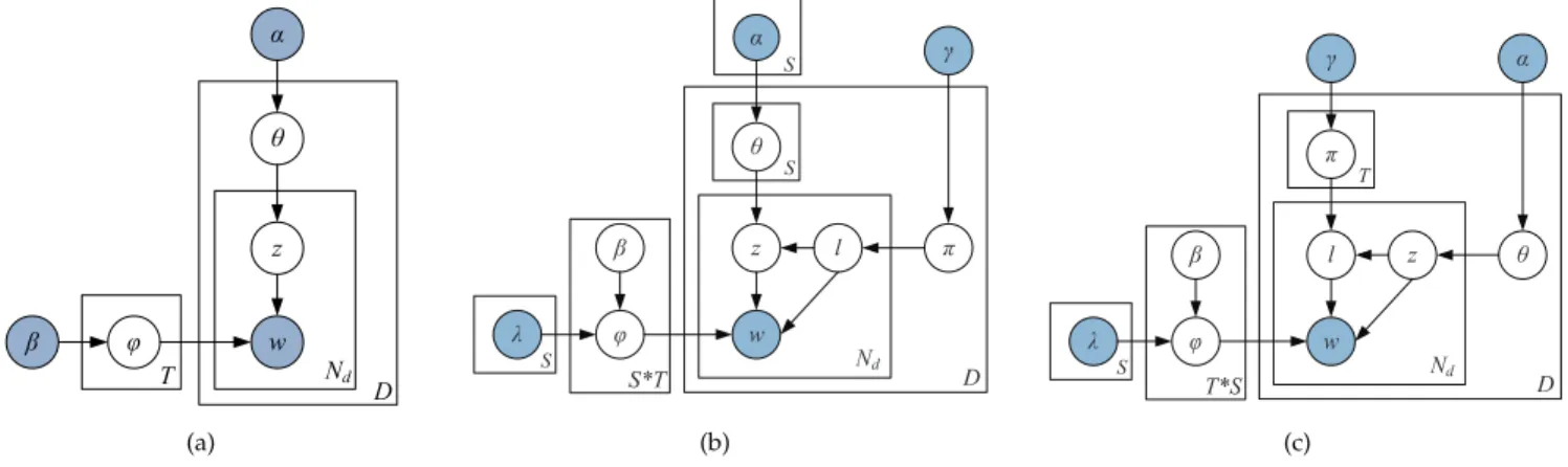
The LDA model, as shown in Figure 1(a), is based upon the assumption that documents are mixture of topics, where a topic is a probability distribution over words [10], [22]. Generally, the procedure of generating a word in a document under LDA can be broken down into two stages. One first chooses a distribution over a mixture of T topics for the document. Following that, one picks up a topic randomly from the topic distribution, and draws a word from that topic according to the corresponding topic-word distribution.
The existing framework of LDA has three hierarchical layers, where topics are associated with documents, and words are associated with topics. In order to model document sentiments, we propose a joint sentiment-topic (JST) model [9] by adding an additional sentiment layer between the document and the topic layer. Hence, JST is effectively a four-layer model, where sentiment labels are associated with documents, under which topics are associated with sentiment labels and words are associ-ated with both sentiment labels and topics. A graphical model of JST is represented in Figure 1(b).
Assume that we have a corpus with a collection of D documents denoted by C = {d1, d2, ..., dD}; each
document in the corpus is a sequence of Nd words
w z N d D T (a) S *T w z l N d D S S S (b) w l z N d D T & ' T *S + S (c)
Fig. 1. (a) LDA model; (b) JST model; (c) Reverse-JST model.
document is an item from a vocabulary index with V distinct terms denoted by {1,2, ..., V}. Also, let S be the number of distinct sentiment labels, and T be the total number of topics. The procedure of generating a word wi in document d under JST boils down to three
stages. First, one chooses a sentiment labellfrom the per-document sentiment distributionπd. Following that, one
chooses a topic from the topic distribution θd,l, where
θd,lis conditioned on the sampled sentiment labell. It is
worth noting that the topic distribution of JST is different from that of LDA. In LDA, there is only one topic distributionθfor each individual document. In contrast, in JST each document is associated with S (number of sentiment labels) topic distributions, each of which corresponds to a sentiment labellwith the same number of topics. This feature essentially provides means for the JST model to predict the sentiment associated with the extracted topics. Finally, one draws a word from the per-corpus word distribution conditioned on both topic and sentiment label. This is again different from LDA that in LDA a word is sampled from the word distribution only conditioned on topic.
The formal definition of the generative process in JST corresponding to the graphical model shown in Figure 1(b) is as follows:
• For each sentiment label l∈ {1, ..., S}
– For each topicj∈ {1, ..., T}, drawϕlj∼Dir(λl×
βT lj).
• For each document d, choose a distribution πd ∼
Dir(γ).
• For each sentiment labellunder documentd, choose a distribution θd,l∼Dir(α).
• For each word wi in documentd
– choose a sentiment labelli∼Mult(πd), – choose a topiczi ∼Mult(θd,li),
– choose a word wi from ϕlizi, a Multinomial
distribution over words conditioned on topiczi
and sentiment labelli.
The hyperparameters α and β in JST can be treated
as the prior observation counts for the number of times topicjassociated with sentiment labellsampled from a
document and the number of times words sampled from topic j associated with sentiment label l, respectively, before having observed any actual words. Similarly, the hyperparameter γ can be interpreted as the prior observation counts for the number of times sentiment labellsampled from a document before any word from the corpus is observed. In our implementation, we used asymmetric prior α and symmetric prior β and γ. In
addition, there are three sets of latent variables that we need to infer in JST, i.e., the per-document sentiment distributionπ, the per-document sentiment label specific topic distribution θ, and the per-corpus joint sentiment-topic word distributionϕ. We will see later in the paper that the per-document sentiment distributionπplays an important role in determining the document sentiment polarity.
Incorporating Model Prior
We modified Phan’s GibbsLDA++ package3 for the im-plementation of JST and Reverse-JST. Compared to the original LDA model, besides adding a sentiment label generation layer, we also added an additional depen-dency link ofϕon the matrixλof sizeS×V, which we used to encode word prior sentiment information into the JST and Reverse-JST models. The matrix λ can be considered as a transformation matrix which modifies the Dirichlet priorsβ of sizeS×T×V, so that the word prior sentiment polarity can be captured.
The complete procedure of incorporating prior knowl-edge into the JST model is as follows. First, λis initial-ized with all the elements taking a value of 1. Then for each term w ∈ {1, ..., V} in the corpus vocabulary and for each sentiment labell∈ {1, ..., S}, ifwis found in the sentiment lexicon, the elementλlw is updated as follows
λlw =
1 if S(w) =l
0 otherwise , (1)
where the functionS(w)returns the prior sentiment label of w in a sentiment lexicon, i.e., neutral, positive or negative. For example, the word “excellent” with index
i in the vocabulary has a positive sentiment polarity. The corresponding row vector in λ is [0,1,0] with its elements representing neutral, positive, and negative prior polarity. For each topic j ∈ {1, ..., T}, multiplying λli with βlji, only the value of βlposji is retained, and
βlneuji andβlnegji are set to 0. Thus, “excellent” can only
be drawn from the positive topic word distributions generated from a Dirichlet distribution with parameter βlpos.
The previously proposed DiscLDA [23] and Labeled LDA [24] also utilize a transformation matrix to modify Dirichlet priors by assuming the availability of docu-ment class labels. DiscLDA uses a class-dependent linear transformation to project a K-dimensional (K latent topics) document-topic distribution into aL-dimensional space (L document labels), while Labeled LDA simply defines a one-to-one correspondence between LDA’s la-tent topics and document labels. In contrast to this work, we use word prior sentiment as supervised information and modify the topic-word Dirichlet priors for sentiment classification.
Model Inference
In order to obtain the distributions of π, θ, and ϕ, we firstly estimate the posterior distribution over z and l, i.e., the assignment of word tokens to topics and sentiment labels. The sampling distribution for a word given the remaining topics and sentiment labels isP(zt=j, lt=k|w,z−t,l−t,α, β, γ), wherez−t andl−t
are vector of assignments of topics and sentiment labels for all the words in the collection except for the word at position tin document d.
The joint probability of the words, topics and senti-ment label assignsenti-ments can be factored into the follow-ing three terms:
P(w,z,l) =P(w|z,l)P(z,l) =P(w|z,l)P(z|l)P(l) (2)
For the first term, by integrating out ϕ, we obtain P(w|z,l) = Γ(V β) Γ(β)V S∗T Y k Y j Q iΓ(Nk,j,i+β) Γ(Nk,j+V β) , (3) where Nk,j,iis the number of times wordi appeared in
topic j and with sentiment label k, Nk,j is the number
of times words assigned to topic j and sentiment label k, andΓ is the gamma function.
For the second term, by integrating out θ, we obtain
P(z|l) = Γ( PT j=1αk,j) QT j=1Γ(αk,j) !D∗S Y d Y k Q jΓ(Nd,k,j+αk,j) Γ(Nd,k+Pjαk,j) , (4) where D is the total number of documents in the collection, Nd,k,j is the number of times a word from
documentdbeing associated with topicj and sentiment labelk, andNd,k is the number of times sentiment label
k being assigned to some word tokens in documentd.
For the third term, by integrating out π, we obtain P(l) = Γ(Sγ) Γ(γ)S D Y d Q kΓ(Nd,k+γ) Γ(Nd+Sγ) , (5)
whereNd is the total number of words in documentd.
Gibbs sampling was used to estimate the posterior distribution by sampling the variables of interest,ztand
lt here, from the distribution over the variables given
the current values of all other variables and data. Letting the superscript−t denote a quantity that excludes data fromtthposition, the conditional posterior for z
tand lt
by marginalizing out the random variables ϕ, θ, and π is P(zt=j, lt=k|w,z− t ,l−t ,α, β, γ)∝ N−t k,j,wt+β N−t k,j+V β · N −t d,k,j+αk,j N−t d,k+ P jαk,j · N −t d,k+γ N−t d +Sγ . (6)
Samples obtained from the Markov chain are then used to approximate the per-corpus sentiment-topic word distribution
ϕk,j,i=
Nk,j,i+β
Nk,j+V β
. (7)
The approximate per-document sentiment label spe-cific topic distribution is
θd,k,j=
Nd,k,j+αk,j
Nd,k+Pjαk,j
. (8)
Finally, the approximate per-document sentiment dis-tribution is
πd,k=
Nd,k+γ
Nd+Sγ
. (9)
The pseudo code for the Gibbs sampling procedure of JST is shown in Algorithm 1.
3.2 Reverse Joint Sentiment-Topic (Reverse-JST) Model
In this section, we studied a reparameterized version of the JST model called Reverse-JST. As opposed to JST in which topic generation is conditioned on senti-ment labels, sentisenti-ment label generation in Reverse-JST is dependent on topics. As shown in Figure 1(c), the Reverse-JST model is a four-layer hierarchical Bayesian model, where topics are associated with documents, under which sentiment labels are associated with topics and words are associated with both topics and sentiment labels. Using similar notations and terminologies as in Section 3.1, the joint probability of the words, the topics and sentiment label assignments of Reverse-JST can be factored into the following three terms:
P(w,l,z) =P(w|l,z)P(l,z) =P(w|l,z)P(l|z)P(z).
(10) It is easy to derive the Gibbs sampling for Reverse-JST in the same way as JST. Therefore, here we only give the
Algorithm 1Gibbs sampling procedure of JST.
Require: α,β,γ, Corpus
Ensure: sentiment and topic label assignment for all word tokens in the corpus
1: InitializeS×T×V matrixΦ,D×S×T matrixΘ,
D×S matrixΠ.
2: fori= 1 tomaxGibbs sampling iterationsdo 3: forall documentsd∈[1, M] do
4: forall wordst∈[1, Nd]do
5: Exclude wordt associated with sentiment la-bel l and topic label z from variables Nk,j,i,
Nk,j,Nd,k,j,Nd,k andNd;
6: Sample a new sentiment-topic pair ˜l and z˜ using Equation 6;
7: Update variablesNk,j,i,Nk,j,Nd,k,j,Nd,k and
Nd using the new sentiment label˜land topic
label˜z;
8: end for 9: end for
10: forevery 25 iterations do
11: Update hyperparameterα with the
maximum-likelihood estimation;
12: end for
13: forevery 100 iterationsdo
14: Update the matrixΦ,Θ, andΠwith new
sam-pling results;
15: end for 16: end for
full conditional posterior for ztand ltby marginalizing
out the random variablesϕ,θ, andπ P(zt=j, lt=k|w,z− t ,l−t ,α, β, γ)∝ N−t j,k,wt+β N−t j,k+V β ·N −t d,j,k+γ N−t d,j+Sγ · N −t d,j+αj N−t d + P jαj . (11) As we do not have a direct per-document sentiment distribution in Reverse-JST, a distribution over senti-ment labels for docusenti-ment P(l|d) is calculated based on
the topic specific sentiment distribution π and the per-document topic proportion θ.
P(l|d) =X
z
P(l|z, d)P(z|d) (12)
4
E
XPERIMENTALS
ETUP 4.1 Datasets DescriptionTwo publicly available datasets, the MR and MDS datasets, were used in our experiments. The MR dataset has become a benchmark for many studies since the work of Pang et al. [3]. The version 2.0 used in our experiment consists of 1000 positive and 1000 negative movie reviews crawled from the IMDB movie archive, with an average of 30 sentences in each document. We also experimented with another dataset, namely subjec-tive MR, by removing the sentences that do not bear opinion information from the MR dataset, following the
approach of Pang and Lee [4]. The resulting dataset still contains 2000 documents with a total of 334,336 words and 18,013 distinct terms, about half the size of the original MR dataset without performing subjectivity detection.
First used by Blitzeret al.[7], the MDS dataset contains 4 different types of product reviews clawed from Ama-zon.com including Book, DVD, Electronics and Kitchen, with 1000 positive and 1000 negative examples for each domain4.
Preprocessing was performed on both of the datasets. Firstly, punctuation, numbers, non-alphabet characters and stop words were removed. Secondly, standard stem-ming was performed in order to reduce the vocabulary size and address the issue of data sparseness. Summary statistics of the datasets before and after preprocessing is shown in Table 1.
4.2 Defining Model Priors
In the experiments, two subjectivity lexicons, namely the MPQA5and the appraisal lexicons6, were combined and incorporated as prior information into the model learn-ing. These two lexicons contain lexical words whose po-larity orientation have been fully specified. We extracted the words with strong positive and negative orientation and performed stemming in the preprocessing. In ad-dition, words whose polarity changed after stemming were removed automatically, resulting in 1584 positive and 2612 negative words, respectively. It is worth noting that the lexicons used here are fully domain-independent and do not bear any supervised information specifically to the MR, subjMR and MDS datasets. Finally, the prior information was produced by retaining all words in the MPQA and appraisal lexicons that occurred in the exper-imental datasets. The prior information statistics for each dataset is listed in Table 2. It can be observed that the prior positive words occur much more frequently than the negative words with its frequency at least doubling that of negative words in all of the datasets.
4.3 Hyperparameter Settings
Previous study has shown that while LDA can produce reasonable results with a simple symmetric Dirichlet prior, an asymmetric prior over the document-topic dis-tributions has substantial advantage over a symmetric prior [25]. In the JST model implementation, we set the symmetric prior β = 0.01 [22], the symmetric prior γ = (0.05×L)/S, where L is the average document length, S the is total number of sentiment labels, and the value of 0.05 on average allocates 5% of probability mass for mixing. The asymmetric prior α is learned 4. We did not perform subjectivity detection on the MDS dataset since its average document length is much shorter than that of the MR dataset, with some documents even containing one sentence only.
5. http://www.cs.pitt.edu/mpqa/
TABLE 1
Dataset statistics. Note:†denotes before preprocessing and * denotes after preprocessing.
Dataset
# of words
MR subjMR MDS
Book DVD Electronics Kitchen Average doc. length† 666 406 176 170 110 93 Average doc. length* 313 167 116 113 75 63 Vocabulary size† 38,906 34,559 22,028 21,424 10,669 9,525 Vocabulary size* 25,166 18,013 19,428 20,409 9,893 8,512
TABLE 2
Prior information statistics. Prior lexicon
MR subjMR MDS
(pos./neg.) Book DVD Electronics Kitchen
No. of distinct 1,248/1,877 1,150/1,667 1,008/1,360 987/1320 571/555 595/514 words
Total 108,576/57,744 67,751/34,276 31,697/14,006 31,498/13,935 19,599/6,245 18,178/6,099 occurrence
Coverage (%) 17/9 20/10 13/6 14/6 13/4 14/5
directly from data using maximum-likelihood estima-tion [26] and updated every 25 iteraestima-tions during the Gibbs sampling procedure. In terms of Reverse-JST, we set the symmetric β = 0.01,γ= (0.05×L)/(T×S), and the asymmetric prior α is also learned from data as in
JST.
4.4 Classifying Document Sentiment
The document sentiment is classified based on P(l|d),
the probability of sentiment label given document. In our experiments, we only consider the probability of positive and negative label given document, with the neutral label probability being ignored. There are two reasons. First, sentiment classification for both the MR and MDS datasets is effectively a binary classification problem, i.e., documents are being classified either as positive or nega-tive, without the alternative of neutral. Second, the prior information we incorporated merely contributes to the positive and negative words, and consequently there will be much more influence on the probability distribution of positive and negative label given document, rather than the distribution of neutral label given document. Therefore, we define that a document d is classified as a positive-sentiment document if its probability of positive sentiment label given document P(lpos|d), is
greater than its probability of negative sentiment label given document P(lneg|d), and vice versa.
5
EXPERIMENTAL
RESULTS
In this section, we present and discuss the experimental results of both document-level sentiment classification and topic extraction, based on the MR and MDS datasets. 5.1 Sentiment Classification Results vs. Number of Topics
As both JST and Reverse-JST model sentiment and mix-ture of topics simultaneously, it is therefore worth
ex-ploring how the sentiment classification and topic extrac-tion tasks affect/benifit each other and in addiextrac-tion, how these two models behave with different topic number settings on different datasets when prior information is incorporated. With this in mind, we conducted a set of experiments on JST and Reverse-JST, with topic number T ∈ {1,5,10,15,20,25,30}. It is worth noting that as JST models the same number of topics under each sentiment label, therefore with three sentiment labels, the total topic number of JST will be equivalent to a standard LDA model withT ∈ {3,15,30,45,60,75,90}.
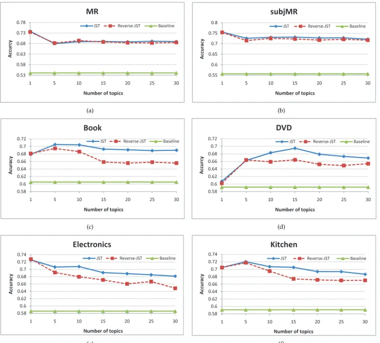
Figure 2 shows the sentiment classification results of both JST and Reverse-JST at document-level by incor-porating prior information extracted from the MPQA and appraisal lexicons. For all the reported results, ac-curacy is used as performance measure and the results were averaged over 10 runs. The baseline is calculated by counting the overlap of the prior lexicon with the training corpus. If the positive sentiment word count is greater than that of the negative words, a document is classified as positive, and vice versa. The improvement over this baseline will reflect how much JST and Reverse-JST can learn from data.
As can be seen from Figure 2 that, both JST and Reverse-JST have a significant improvement over the baseline in all of the datasets. When the topic number is set to 1, both JST and Reverse-JST essentially become the standard LDA model with only three sentiment topics, and hence ignores the correlation between sentiment labels and topics. Figure 2(c), 2(d) and 2(f) show that, both JST and Reverse-JST perform better with multiple topic settings in the Book, DVD and Kitchen domains, especially noticeable for JST with 10% improvement at T = 15 over single topic setting on the DVD domain. This observation shows that modelling sentiment and topics simultaneously indeed help improve sentiment classification. For the cases where single topic performs the best (i.e., Figure 2(a), 2(b) and 2(e)), it is observed that
0.53 0.58 0.63 0.68 0.73 0.78 1 5 10 15 2 0 25 3 0 Ac c u rc y N u m b e r of top ics M R JST Reverse%JST Baseline (a) 0.55 0.6 0.65 0.7 0.75 0.8 1 5 10 15 20 25 30 Ac c u r ac y N u m b er of to p ics s u b jM R JST ReverseUJST Baseline (b) 0.5 8 0.6 0.6 2 0.6 4 0.6 6 0.6 8 0.7 0.7 2 1 5 10 15 20 25 30 Ac u r ac y N u m b e r ofto p ics B o o k JST R everseJST Baseline (c) 0.5 8 0.6 0.6 2 0.6 4 0.6 6 0.6 8 0.7 0.7 2 1 5 10 15 20 25 30 Ac c u rc y N u m b er of to p ics D V D JST Reverse¯JST Baseline (d) 0.58 0.6 0.62 0.64 0.66 0.68 0.7 0.72 0.74 1 5 10 15 20 25 30 Ac c u r ac y N u m b e r of to p ics E le c t ro n ic s JST ReverseäJST Baseline (e) 0.58 0 .6 0.62 0.64 0.66 0.68 0 .7 0.72 0.74 1 5 10 15 20 25 30 Ac c u r ac y N u m b er of to p ics K it c h e n JST ReverseJST Baseline (f)
Fig. 2. Sentiment classification accuracy VS. different topic number settings.
apart from the MR dataset, the drop in sentiment clas-sification accuracy by additionally modelling mixture of topics is only marginal (i.e., 1% and 2% point drop in subjMR and Electronics, respectively), but both JST and Reverse-JST are able to extract sentiment-oriented topics in addition to document-level sentiment detection.
When comparing JST with Reverse-JST, there are three observations: (1) JST outperforms Reverse-JST in most of the datasets with multiple topic settings, with up to 4% difference in the Book domain; (2) the performance difference between JST and Reverse-JST has some corre-lation with the corpus size (cf. Table 1). That is when the corpus size is large, these two models perform almost the same, e.g., on the MR dataset. In contrast, when the cor-pus size is relatively small, JST significantly outperforms Reverse-JST, e.g., on the MDS dataset. A significance
measure based on paired t-Test (critical P = 0.05) is reported in Table 3 ; (3) for both models, the sentiment classification accuracy is less affected by topic number settings when the dataset size is large. For instance, classification accuracy stays almost the same for the MR and subjMR datasets when topic number is increased from 5 to 30, whereas in contrast, 2-3% drop is observed for Electronics and Kitchen. By closely examining the posterior of JST and Reverse-JST (cf. Equation 6 and 11), we noticed that the count Nd,j (number of times topic
j associated with some word tokens in document d) in the Reverse-JST posterior would be relatively small due to the factor of a large topic number setting. On the con-trary, the countNd,k (number of times sentiment labelk
assigned to some word tokens in documentd) in the JST posterior would be relatively large as k is only defined
TABLE 3
Significant test results. Note: blank denotes the performance of JST and Reverse-JST is significantly undistinguishable; * denotes JST significantly outperforms Reverse-JST.
T MR subjMR Book DVD Electronics Kitchen 5 10 * 15 * * * * 20 * * * * 25 * * * * * 30 * * *
over 3 different sentiment labels. This essentially makes JST less sensitive to the data sparseness problem and the perturbation of hyperparameter settings. In addition, JST encodes the assumption that there is approximately a single sentiment for the entire document, i.e., documents are mostly either positive or negative. This assumption is important as it allows the model to cluster different terms which share similar sentiment. In Reverse-JST, this assumption is not enforced unless only one topic for each sentiment label is defined. Therefore, JST appears to be a more appropriate model design for joint sentiment topic detection.
5.2 Comparison with Existing Models
In this section, we compare the overall sentiment clas-sification performance of JST, Reverse-JST with some existing semi-supervised approaches [19], [27]. As can be seen from Table 4 that, the baseline results calcu-lated based on the sentiment lexicon are below 60% for most of the datasets. By incorporating the same prior lexicon, a significant improvement is observed for JST and Reverse-JST over the baseline, where both models have over 20% performance gain on the MR and subjMR datasets, and 10-14% improvement on the MDS dataset. For the movie review data, there is a further 2% improvement for both models on the subjMR dataset over the original MR dataset. This suggests that though the subjMR dataset is in a much compressed form, it is more effective than the full dataset as it retains compa-rable polarity information in a much cleaner way [4]. In terms of the MDS dataset, both JST and Reverse-JST perform better on Electronics and Kitchen than Book and DVD, with about 2% difference in accuracy. Manually analyzing the MDS dataset reveals that the book and DVD reviews often contain a lot of descriptions of book contents or movie plots, which makes the reviews of these two domains difficult to classify; in contrast, in Electronics and Kitchen, comments on products are often expressed in a much more straightforward manner. In terms of the overall performance, except in Electronics, it was observed that JST performed slightly better than Reverse-JST in all sets of experiments, with differences of 0.2-3% being observed.
When compared to the recently proposed weakly-supervised approach based on a spectral clustering al-gorithm [27], except slightly lower in the DVD domain,
JST achieved better performance in all the other domains with more than 3% overall improvement. Nevertheless, the proposed approach [27] requires users to specify which dimensions (defined by the eigenvectors in spec-tral clustering) are most closely related to sentiment by inspecting a set of features derived from the reviews for each dimension, and clustering is performed again on the data to derive the final results. In contrast, for the JST and Reverse-JST models proposed here, no hu-man judgement is required. Another recently proposed non-negative matrix tri-factorization approach [19] also employed lexical prior knowledge for semi-supervised sentiment classification. However, when incorporating 10% of labelled documents for training, the non-negative matrix tri-factorization approach performed much worse than JST, with only around 60% accuracy being achieved for all the datasets. Even with 40% labelled documents, it still performs worse than JST on the MR dataset and only slightly outperforms JST on the MDS dataset. It is worth noting that no labelled documents were used in the JST results reported here.
5.3 Sentiment Classification Results with Different Features
While JST and Reverse-JST models can give better or comparative performance in document-level senti-ment classification compared to semi-supervised ap-proaches [19], [27] with unigram features, it is worth considering the dependency between words since it might serve an important function in sentiment analy-sis. For instance, phrases expressing negative sentiment such as “not good” or “not durable” will convey com-pletely different polarity meaning without considering negations. Therefore, we extended the JST and Reverse-JST models to include higher order information, i.e., bigrams, for model learning. Table 5 shows the feature statistics of the datasets in unigrams, bigrams and the combination of both. For the negator lexicon, we collect a handful of words from the General Inquirer under the NOTLWcategory7. We experimented with topic number T ∈ {1,5,10,15,20,25,30}. However, it was found that JST and Reverse-JST achieved best results with single topic on bigrams and the combination of bigrams and unigrams most of the time, except a few cases where
TABLE 4
Performance comparison with existing models. (Note: boldface denotes the best results.) Aaccuracy (%)
MR subjMR Book DVD ElectronicsMDSKitchen MDS overall
Baseline 54.1 55.7 60.6 59.2 58.6 59.1 59.4
JST 73.9 75.6 70.5 69.5 72.6 72.1 71.2
Reverse-JST 73.5 75.4 69.5 66.4 72.8 71.7 70.1 Dasgupta and Ng (2009) 70.9 N/A 69.5 70.8 65.8 69.7 68.9 Li et al.(2009) with 10% doc. label 60 N/A
N/A 62
Li et al.(2009) with 40% doc. label 73.5 N/A 73 TABLE 5
Unigram and bigram features statistics. # of features (Unit: thousand)
Dataset MR subjMR Book DVD ElectronicsMDS Kitchen
unigrams 626 334 232 226 150 126
bigrams 1,239 680 318 307 201 170 unigrams+bigrams 1,865 1,014 550 533 351 296
TABLE 6
Sentiment classification results with different features. Note: boldface denotes the best results. Accuracy(%)
JST Reverse-JST
unigrams bigrams unigrams+bigrams unigrams bigrams unigrams+bigrams
MR 73.9 74 76.6 73.5 74.1 76.6 subjMR 75.6 75.6 77.7 75.4 75.5 77.6 Book 70.5 70.3 70.8 69.5 69.7 69.8 DVD 69.5 71.3 72.5 66.4 71.4 72.4 Electronics 72.6 70.2 74.9 72.8 70.5 75 Kitchen 72.1 70 70.8 71.7 69.9 70.5
multiple topics perform better (i.e., JST and Reverse-JST with T = 5 on Book using unigrams+bigrams, as well as Reverse-JST with T = 10 on Electronics using unigrams+bigrams). This is probably due to the fact that bigrams features have much lower frequency counts than unigrams. Thus, with the sparse feature co-occurrence, multiple topic settings likely fail to cluster different terms that share similar sentiment and hence harm the sentiment classification accuracy.
Table 6 shows the sentiment classification results of JST and Reverse-JST with different features being used. It can be observed that both JST and Reverse-JST perform almost the same with unigrams or bigrams on the MR, subjMR, and Book datasets. However, using bigrams gives a better accuracy in DVD but is worse on Electron-ics and Kitchen compared to using unigrams for both models. When combining both unigrams and bigrams, a performance gain is observed for most of the datasets except the Kitchen data. For both MR and subjMR, using the combination of unigrams and bigrams gives more than 2% improvement compared to using either unigrams or bigrams alone, with 76.6% and 77.7% accu-racy being achieved on these two datasets, respectively. For the MDS dataset, the combined features slightly outperforms unigrams and bigrams on Book and gives a significant gain on DVD (i.e., 3% over unigrams; 1.2%
over bigrams) and Electronics (i.e., 2.3% over unigrams; 4.7% over bigrams). Thus, we may conclude that the combination of unigrams and bigrams gives the best overall performance.
5.4 Topic Extraction
The second goal of JST is to extract topics from the MR (without subjectivity detection) and MDS datasets, and evaluate the effectiveness of topic sentiment captured by the model. Unlike the LDA model where a word is drawn from the topic-word distribution, in JST one draws a word from the per-corpus word distribution conditioned on both topics and sentiment labels. There-fore, we analyze the extracted topics under positive and negative sentiment label, respectively. 20 topic examples extracted from the MR and MDS datasets are shown in Table 7, where each topic was drawn from a particular domain under a sentiment label.
Topics on the top half of Table 7 were generated under the positive sentiment label and the remaining topics were generated under the negative sentiment label, each of which is represented by the top 15 topic words. As can be seen from the table that the extracted topics are quite informative and coherent. The movie review topics try to capture the underlying theme of a movie or the relevant comments from a movie reviewer, while
TABLE 7
Topic examples extracted by JST under different sentiment labels.
MR Book DVD Electronics Kitchen
P o si ti v e se n ti m en t la b el
ship good recip children action funni mous sound color recommend
titan realli food learn good comedi hand qualiti beauti highli
crew plai cook school fight make logitech stereo plate impress
cameron great cookbook child right humor comfort good durabl love
alien just beauti ag scene laugh scroll high qualiti favorit
jack perform simpl parent chase charact wheel listen fiestawar especi
water nice eat student hit joke smooth volum blue nice
stori fun famili teach art peter feel decent finger beautifulli
rise lot ic colleg martial allen accur music white absolut
rose act kitchen think stunt entertain track hear dinnerwar fabul
boat direct varieti young chan funniest touch audio bright bargin
deep best good cours brilliant sweet click set purpl valu
ocean get pictur educ hero constantli conveni price scarlet excel
dicaprio entertain tast kid style accent month speaker dark bought
sink better cream english chines happi mice level eleg solid
N eg at iv e se n ti m en t la b el
prison bad polit war horror murder drive batteri fan amazon
evil worst east militari scari killer fail charg room order
guard plot middl armi bad cop data old cool return
green stupid islam soldier evil crime complet life air ship
hank act unit govern dead case lose unaccept loud sent
wonder suppos inconsist thing blood prison failur charger nois refund
excute script democrat evid monster detect recogn period live receiv
secret wast influenc led zombi investig backup longer annoi damag
mile dialogu politician iraq fear mysteri poorli recharg blow dissapoint
death bore disput polici scare commit error hour vornado websit
base poor cultur destruct live thriller storag last bedroom discount
tom complet eastern critic ghost attornei gb power inferior polici
convict line polici inspect devil undercov flash bui window unhappi
return terribl state invas head suspect disast worthless vibrat badli franklin mess understand court creepi shock yesterdai realli power shouldn
the topics from the MDS dataset represent a certain product review from the corresponding domain. For example, for the two positive sentiment topics under the movie review domain, the first is closely related to the very popular romantic movie“Titanic”directed by James Cameron and casted by Leonardo DiCaprio and Kate Winslet, whereas the other one is likely to be a positive review for a movie. Regarding the MDS dataset, the first topic of Book and DVD under the positive sentiment label probably discusses a good cookbook and a popular action movie by Jackie Chan, respectively; for the first negative topic of Electronics, it is likely to be complaints regarding data loss due to the flash drive failure, while the first negative topic of the kitchen domain is probably the dissatisfaction of the high noise level of the Vornado brand fan.
In terms of topic sentiment, by examining each of the topics in Table 7, it is quite evident that most of the positive and negative topics indeed bear positive and negative sentiment, respectively. The first movie review topic and the second Book topic under the positive senti-ment label mainly describes movie plot and the contents of a book, with less words carrying positive sentiment compared to other positive sentiment topics under the same domain. Manually examining the data reveals that the terms that seem not conveying sentiments under the topic in fact appears in the context expressing positive sentiments. Overall, the above analysis illustrates the effectiveness of JST in extracting opinionated topics from a corpus.
6
CONCLUSIONS AND
FUTURE
WORK
In this paper, we presented a joint sentiment-topic (JST) model and a reparameterized version of JST called Reverse-JST. While most of the existing approaches to sentiment classification favor in supervised learning, both JST and Reverse-JST models target sentiment and topic detection simultaneously in a weakly-supervised fashion. Without hierarchical prior, JST and Reverse-JST are essentially equivalent. However, extensive experi-ments conducted on datasets across different domains reveal that, these two models behave very differently when sentiment prior knowledge is incorporated, where JST consistently outperformed Reverse-JST. For general domain sentiment classification, by incorporating a small amount of domain-independent prior knowledge, the JST model achieved either better or comparable perfor-mance compared to existing semi-supervised approaches despite using no labelled documents, which demon-strates the flexibility of JST in the sentiment classification task. Moreover, the topics and topic sentiments detected by JST are indeed coherent and informative.
There are several directions we plan to investigate in the future. One is incremental learning of the JST parameters when facing with new data. Another one is the modification of the JST model with other supervised information being incorporated into JST model learning, such as some known topic knowledge for certain product reviews or document labels derived automatically from the user supplied review ratings.
A
CKNOWLEDGMENTSWe would like to thank the anonymous reviewers for their valuable comments.
REFERENCES
[1] B. Pang and L. Lee, “Opinion mining and sentiment analysis,”
Found. Trends Inf. Retr., vol. 2, no. 1-2, pp. 1–135, 2008.
[2] P. D. Turney, “Thumbs up or thumbs down?: semantic orientation applied to unsupervised classification of reviews,” inProceedings of ACL, 2001, pp. 417–424.
[3] B. Pang, L. Lee, and S. Vaithyanathan, “Thumbs up?: sentiment classification using machine learning techniques,” inProceedings of EMNLP, 2002, pp. 79–86.
[4] B. Pang and L. Lee, “A sentimental education: sentiment analysis using subjectivity summarization based on minimum cuts,” in
Proceedings of ACL, 2004, p. 271.
[5] C. Whitelaw, N. Garg, and S. Argamon, “Using appraisal groups for sentiment analysis,” inProceedings of CIKM, 2005.
[6] A. Kennedy and D. Inkpen, “Sentiment classification of movie re-views using contextual valence shifters,”Computational Intelligence, vol. 22, no. 2, pp. 110–125, 2006.
[7] J. Blitzer, M. Dredze, and F. Pereira, “Biographies, bollywood, boom-boxes and blenders: Domain adaptation for sentiment clas-sification,” inProceedings of ACL, 2007, pp. 440–447.
[8] A. Aue and M. Gamon, “Customizing sentiment classifiers to new domains: a case study,” inProceedings of RANLP, 2005.
[9] C. Lin and Y. He, “Joint sentiment/topic model for sentiment analysis,” inProceedings of CIKM, 2009.
[10] D. M. Blei, A. Y. Ng, and M. I. Jordan, “Latent Dirichlet alloca-tion,”J. Mach. Learn. Res., vol. 3, pp. 993–1022, 2003.
[11] Q. Mei, X. Ling, M. Wondra, H. Su, and C. Zhai, “Topic sentiment mixture: modeling facets and opinions in weblogs,” inProceedings of WWW, 2007, pp. 171–180.
[12] I. Titov and R. McDonald, “A joint model of text and aspect ratings for sentiment summarization,” inProceedings of ACL-HLT, 2008, pp. 308–316.
[13] S. Hayakawa and E. Ehrlich,Choose the right word: A contemporary guide to selecting the precise word for every situation. Proceedings of Collins, 1994.
[14] S. Li and C. Zong, “Multi-domain sentiment classification,” in
Proceedings of ACL-HLT, 2008, pp. 257–260.
[15] R. McDonald, K. Hannan, T. Neylon, M. Wells, and J. Reynar, “Structured models for fine-to-coarse sentiment analysis,” in Pro-ceedings of ACL, 2007, pp. 432–439.
[16] A. Abbasi, H. Chen, and A. Salem, “Sentiment analysis in mul-tiple languages: Feature selection for opinion classification in web forums,”ACM Trans. Inf. Syst., vol. 26, no. 3, pp. 1–34, 2008. [17] N. Kaji and M. Kitsuregawa, “Automatic construction of
polarity-tagged corpus from html documents,” in Proceedings of COL-ING/ACL, 2006, pp. 452–459.
[18] A. Andreevskaia and S. Bergler, “When specialists and general-ists work together: Overcoming domain dependence in sentiment tagging,” inProceedings of ACL-HLT, 2008, pp. 290–298.
[19] T. Li, Y. Zhang, and V. Sindhwani, “A non-negative matrix tri-factorization approach to sentiment classification with lexical prior knowledge,” inProceedings of ACL-IJCNLP, 2009, pp. 244–252. [20] I. Titov and R. McDonald, “Modeling online reviews with
multi-grain topic models,” inProceedings of WWW, 2008.
[21] T. Hofmann, “Probabilistic latent semantic indexing,” in Proceed-ings of SIGIR, 1999, pp. 50–57.
[22] M. Steyvers and T. Griffiths, “Probabilistic Topic Models,” Hand-book of Latent Semantic Analysis, p. 427, 2007.
[23] S. Lacoste-Julien, F. Sha, and M. Jordan, “DiscLDA: Discrimina-tive learning for dimensionality reduction and classification,” in
Proceedings of NIPS, 2008.
[24] D. Ramage, D. Hall, R. Nallapati, and C. Manning, “Labeled LDA: A supervised topic model for credit attribution in multi-labeled corpora,” inProceedings of EMNLP, 2009, pp. 248–256.
[25] H. Wallach, D. Mimno, and A. McCallum, “Rethinking LDA: Why priors matter,” inTopic Models: Text and Beyond Workshop in Neural Information Processing Systems Conference, 2009.
[26] T. Minka, “Estimating a Dirichlet distribution,” MIT, Tech. Rep., 2003.
[27] S. Dasgupta and V. Ng, “Topic-wise, Sentiment-wise, or Other-wise? Identifying the Hidden Dimension for Unsupervised Text Classification,” inProceedings of EMNLP, 2009, pp. 580–589.
PLACE PHOTO HERE
Chenghua Lin is currently a PhD student
in Computer Science, College of Engineering, Mathematics and Physical Sciences at the Uni-versity of Exeter. He received his BEng degree in Electrical Engineering and Automation from Beihang University in 2006, China, and MEng degree (1st class Honors) in Electronic Engi-neering from the University of Reading in 2007, UK. His research interests are sentiment anal-ysis of web data using machine learning and statistical methods.
PLACE PHOTO HERE
Yulan He received the BASc (1st class Honors)
and MEng degrees in Computer Engineering from Nanyang Technological University, Singa-pore, in 1997 and 2001, respectively, and the PhD degree in 2004 from Cambridge University Engineering Department, UK. She is currently a Senior Lecturer at the Knowledge Media In-stitute of the Open University, UK. Her early research focused on spoken language under-standing, biomedical literature mining, and mi-croarray data analysis. Her current research in-terests lie in the integration of machine learning and natural language processing for sentiment analysis and information extraction from the Web.
PLACE PHOTO HERE
Richard Everson graduated with a degree in
Physics from Cambridge University in 1983 and a PhD in Applied Mathematics from Leeds Uni-versity in 1988. He worked at Brown and Yale Universities on fluid mechanics and data analy-sis problems until moving to Rockefeller Univer-sity, New York to work on optical imaging and modelling of the visual cortex. After working at Imperial College, London, he joined the Com-puter Science department at Exeter University where he is now an Associate Professor of Machine Learning. Current research interests are in statistical pattern recognition, multi-objective optimisation and the links between them.
PLACE PHOTO HERE
Stefan R ¨uger (Dr rer nat Dipl-Phys FHEA
MACM MBCS) joined The Open University’s Knowledge Media Institute in 2006 to take up a chair in Knowledge Media and head a research group working on Multimedia Information Re-trieval. Before that he was a Reader in Multime-dia and Information Systems at the Department of Computing, Imperial College London, where he also held an EPSRC Advanced Research Fellowship (1999-2004). Rger is a theoretical physicist by training (FU Berlin) and received his PhD in the field of computing for his work on artificial intelligence and, in particular, the theory of neural networks from TU Berlin in 1996. For further information and publications see http://kmi.open.ac.uk/mmis.