Texture Classification of lung computed tomography (CT) using local binary patterns (LBP)

(1)

Texture Classification of lung computed tomography (CT)

using local binary patterns (LBP)

by

MOHAMAD AFIF SYAUQI BIN MOHD YUSRI 14757

Submitted to the Department of Electrical & Electronics Engineering in Partial Fulfillment of the Requirements

for the Degree

Bachelor of Engineering (Hons) (Electrical & Electronics Engineering)

JANUARY 2015

Universiti Teknologi PETRONAS Bandar Seri Iskandar

32610 Tronoh Perak Darul Ridzuan

(2)

i

CERTIFICATION OF APPROVAL

Texture Classification of lung computed tomography (CT)

using local binary patterns (LBP)

by

MOHAMAD AFIF SYAUQI BIN MOHD YUSRI 14757

A project dissertation submitted to the

Department of Electrical and Electronics Engineering Universiti Teknologi PETRONAS

in partial fulfillment of the requirement for Bachelor of Engineering (Hons) (Electrical and Electronics Engineering)

Approved by,

___________________________ Norashikin Binti Yahya

Project Supervisor

UNIVERSITI TEKNOLOGI PETRONAS TRONOH, PERAK

(3)

ii

CERTIFICATION OF ORIGINALITY

This is to certify that I am responsible for the work submitted in this project, the original work is my own accept as specified in the references and acknowledgements, and that the original work

contained herein have not been undertaken or done by unspecified source of persons.

____________________

(4)

iii

ABSTRACT

Emphysema is a type of lung disease and those who suffering from it usually have breathing difficulty. Early detection using CT scan image can save life of many emphysema patient as well as assist medical practitioners in planning suitable treatment to patient. The CT scan of lung gives lung images taken from 3 directions; top, bottom, and center. From the slices, the medical practitioners can monitor the slices with unhealthy tissues and perform further examination. Texture classification and analysis is very important in assisting medical practitioners in diagnosis of emphysema of CT scan. In this work, we proposed an LBP-based lung classification algorithm. The local binary pattern (LBP) is one of the feature extraction technique that can be used in classify the image. Four type of LBP are used for extracting the lung feature.

The derivatives other than the conventional one are Center Symmetric Local Binary Pattern (CS-LBP), Local Binary Pattern Variance (LBPV) and Completed Local Binary Pattern (LBPV). The main idea of LBP is such that the LBP operator will extract the image feature and express it in form of a histogram. Different derivatives of LBP will give different type of histogram of an image. To evaluate the performance of different LBPs, k-NN classifier is used to classifier the CT images to two different classes, normal tissue and abnormal tissue. From evaluation studies of different type LBP-based classification algorithm, it is shown that among the four LBP, CSLBP gives the highest classification accuracy, of 73.58%. This follows with LBP and CLBP at 66.03% and lastly LBPV at 62.26%.

(5)

iv

ACKNOWLEDGEMENT

First and foremost, I would like to express my gratitude to Allah for his guidance and blessing for me to complete my final year project. I also would like to dedicate my special thanks to my wonderful parents, Mohd Yusri Bin Md Daud and Suriyati Binti Sabar for their endless support in all my decisions; in them I have and will always find comfort. I would like to thank my family for giving me support throughout this final year. Thus, give me strength to finish this final year project successfully.

My acknowledgements of thankfulness to my supervisor, Ms. Norashikin Binti Yahya for trusting me to complete this project. I have been inspired by her honesty, intelligence and grace. I owe gratitude to her as her unwavering commitment to me for this final year project. Thank you for the supportive nature and for the concern for my professional and personal well-being. I am very lucky to have her as my supervisor. She has done a lot of things to help me in this project.

Not forgetting to all my friends that assist me in this project and thank you for their unstoppable support to me for every problem that I faced through this project. I end my acknowledgement to everyone that contributes directly and indirectly in my successfulness in order to complete this final year project. Without them, I would not be able to accomplish my final year project entitled “Texture Classification of lung computed tomography (CT) using local binary patterns (LBP)”

(6)

v

LIST OF FIGURES

Figure 1: Effect of rotation on LBP operator 3

Figure 2: Cropping of lung tissue 4

Figure 3: Transitions of pixel 8

Figure 4: k-NN classifier representation 10

Figure 5: The representation of LBP 12

Figure 6: The image of histogram (LBP model) 13

Figure 7: k-NN classifier 13

Figure 8: Flow of LBP process 14

Figure 9: Lung CT scan images 15

Figure 10: General work flow of conducting experiment 16

LIST OF TABLES

Table 1: List of patches for the database 18

Table 2: List of the results of LBP with emphysema database 21 Table 3:- List of the results of CLBP with emphysema database 22 Table 4:- List of the results of LBPV with emphysema database 23 Table 5:- List of the results of CSLBP with emphysema database 24

(9)

viii

LIST OF ABBREVIATIONS

UTP Universiti Teknologi PETRONAS

LBP Local Binary Pattern

CS-LBP Center-Symmetric Local Binary Pattern

LBPV Local Binary Pattern Variance

(10)

Chapter 1: Introduction

1

CHAPTER 1 INTRODUCTION 1 Introduction

In this chapter, the contents are discussing about the objectives and scope of the projects. The ideas of the techniques are related with the problem statements and the objectives. The progress report is the continuation of the previous interim report. A lot of additional information will be added inside the progress report. However, the main chapter for this report is the results part where we want to see what local binary patterns (LBP) can do for this project.

1.1 Background

Emphysema is a type of chronic obstructive pulmonary disease (COPD). People with emphysema have difficulty in blowing air out from their lungs because of the lung tissue has been damaged by several factors. Sometimes, the other symptoms can be seen if someone has shortness of breath, heavy cough or sputum production. The other names of this disease also known as chronic obstructive lung disease (COLD), and chronic obstructive airway disease (COAD) [1]. There will be several type of diagnosis that can be done to measure the severity of the emphysema. For example, spirometry test, x-ray computed tomography (CT), etc. The CT is a common diagnosis that been used widely in the medication area. To describe the image or patterns of the CT, the ability of detecting, classifying and quantifying of lung composition is very crucial in order to get the great outcome from the computer [2].A radiologist relies on the analysis of CT to find the severity of emphysema for making decisions about the diagnosis [2].Therefore, it is very important to have accurate texture analysis techniques to characterize the emphysema morphology patterns.

The patterns of emphysema can be classified as normal tissue (NT), centrilobular emphysema (CLE), paraseptal emphysema (PSE), or panlobular emphysema (PLE) as well as the associated severity [3].There is a procedure to detect the emphysema morphology. The texture classifications of lung procedure identify texture features by extracting the patches of the lung slices. These features are then used to search for other images with matching features.

(11)

2 The appearance method does operate in a few techniques in order to identify the severity of the disease. One of the techniques for the texture analysis is Local Binary Pattern (LBP). This technique had been proposed by Ojala et al [4]. LBP have shown promising results in various applications in computer vision and have successfully been applied in a small number of other medical image analysis tasks, e.g., in mammographic mass detection [5] and magnetic resonance image analysis of the brain [6]. This paper will show the study lung CT texture classification based on LBP. Although there are some techniques that can be used in doing the analysis, LBP has shown a great performance in some texture analysis like face recognition, finger print detection, floor classification and etc.

In [7], Sorenson et al proposed emphysema classification technique based on joint LBP and intensity histogram with k-nearest neighbour as the classifier. The proposed method achieved classification accuracy of 95.2%. However, to achieve the correct classification, several different approach of LBP have to be used. A lot of literature discussing about the texture detection with different approaches. For example, Sallas and Hille using the filter banks to see features classification and detection. The co-occurrence matrix and statistics also gain an attention in features detection (Haralick, 1979). People starts to follow the techniques with varies modification to see the accuracy of the method.

In this report, only LBP will be used to see the effectiveness in the classification of lung tissues. An early conclusion can be made in this experiment which is the techniques can show a good performance in classifying the images. Ojala et al in his papers has shown that the LBP can be computed in a simple way and can be modified to see the results in a tremendous way. However, due to the variation of the textures or images the LBP operator might not works correctly. Under some issues, LBP will definitely fail to determine the classification or recognize the images correctly. Figure 1 is illustrating the effect of rotational images where the LBP might not work accordingly. Due to the rotational effect, LBP can have different value even though the images are same based on the neighbour value which will be explained more in the literature review.

(12)

3 Figure 1: Effect of rotation on LBP operator (a) The image (top) and 90° counter clockwise rotated image (bottom), (b) In the rotated images the neighborhood is rotated counter clockwise by 90°, (c) Values above threshold are shown in red color,(d) The weights corresponding to the threshold neighbors, (e) LBP values.

In other hands, the modification of images or textures can be varied depending on the type of the experiment. The brightness, contrast, and colours of the textures can be a factor to see the changing of the LBP’s value. Therefore, the accuracy of LBP can be changed depending on the characteristics of the images or textures. In this experiment, we try not to change the original spatial algorithm of the CT scan features in order to get the pure results without editing the features.

(13)

4

1.2 Problem Statement

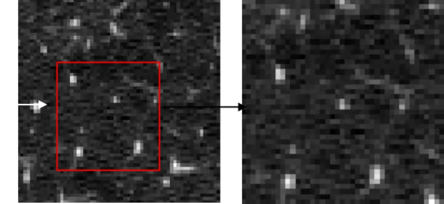
Texture classifications of emphysema from chest CT scans are importance in assisting medical practitioner in monitoring the effect of treatment. In this work, LBP (Local Binary Pattern) will be used to extract the features from CT scan images before being input to a specific classifier. A linear discriminant classifier were been used to classify each image as emphysema (disease) or normal lung. There are two types of databases, slices and patches database. The slices is where the whole lungs can be viewed by medical practitioner which consists of top, center and bottom view of the lungs.

a A0024_top b patch74 c patch74 (crop)

Figure 2: Cropping of lung tissue (patch) (a) top view of lung slice, (b) a patch from the lung slice, (c) cropped version of patch.

From figure 2, the slice is from the top view. From the red circle, the effect of Centrilobular Emphysema (CLE) can be seen. A patch can be produced in order to have detail analysis. The patch need to be cropped in order to have lung texture without any bone scan. The steps in collecting the information for the database is not really convincing since the cropped version of patches will have different spatial algorithm since the pixel for cropped version has been reduced. Therefore, some modification has been made especially for the database where we stick not to crop the patches.

(14)

5

1.3 Objectives & Scope

The project is relevant to be done because the project is under intelligent and imaging signal cluster which is one of the core courses in UTP. As been explained, this project does give an advantage to the people who are researching about LBP in texture analysis and can be contributed to the medical area. Texture classification of lung computed tomography is very important in order to seek the level of severity on the lung disease. Throughout this project, LBP technique will be derive with the different types of lungs.

This project is feasible to be complete within the two semesters. This project potential to get ready with the working code as the techniques had been proved as the easiest the techniques in order to prove the algorithm. There are also equations that had been deriving along with the LBP techniques [12]. All the calculation and simulation need to compare and make it simultaneously in order get the result.

Two objectives need to be achieved at the end of the project. The objectives are as below: o To develop LBPs-based emphysema classification of lung CT scan

o To evaluate the accuracy of the proposed algorithm

In lung texture classification, the details of the texture are very important to represent the severity of the lung disease and for classification of lung tissues. Based on the introduction, there were several techniques of imaging to get the lung texture details. In this review, there will be an overview section about local binary patterns (LBP) and comparison of local binary patterns (LBP) with other techniques or approaches.

(15)

Chapter 2: Literature Review

6

CHAPTER 2 LITERATURE REVIEW

2 Literature Review

Literature review is quite important in any experiments or projects that involving academic matters. From the literature based items, the researchers or evaluators can understand the fundamental and basics of a certain projects and experiments. Furthermore, to collect the information of the literature, that person have to play a role by reading a lot of journal, articles, and research papers.

For this projects, the author has research about the LBP (local binary pattern), CSLBP (center symmetric local binary pattern), LBPV (local binary pattern variance), and CLBP (completed local binary pattern). For the comparison of the texture, kNN (k-nearest neighbor) has been used as the classifier to compare which class does the texture belongs to.

2.1 Techniques

2.1.1 LBP - Local Binary Pattern

The techniques that been used was been proposed by Ojala et. al. for the texture analysis of lungs. The local binary pattern (LBP) is a technique that converts an image into a set of arrays or an array to describe the small-scale appearance of the image [6]. The images later will be analysed by the statistical approaches or histograms.

According to the M. Pietikäinen et al in their book Computer Vision Using Local Binary Patterns [4] , local binary patterns work in the block of an image. The pixel size for the image is 3 x 3 and the centre of it is verge, times to the power of two. To get the value on labelling of the pixel (center), summation of the pixel must be done. For example, (P,R) = (8,1) means 8 pixel for 1 radius of an image [7].Some fundamental equations of local binary pattern (LBP) need to be known before being proceed to the other techniques of local binary pattern (LBP).

Assume gc gray value for center pixel and gp gray values for the sampling points. P stands

for the number of sampling points, and R is the radius of the pixel’s block.

(16)

Chapter 2: Literature Review 7 𝒈𝒑 = 𝒍(𝒙𝒑, 𝒚𝒑), 𝒑 = 𝟎, … , 𝑷 − 𝟏 ___ (2) 𝒙𝒑 = 𝒙 + 𝑹 𝐜𝐨𝐬(𝟐𝝅𝒑 𝑷 ) ___ (3) 𝒚𝒑 = 𝒚 − 𝑹 𝐬𝐢𝐧(𝟐𝝅𝒑 𝑷 ) ___ (4) If gc = (0, 0) 𝒙𝒑 = 𝑹 𝐜𝐨𝐬(𝟐𝝅𝒑 𝑷 ) 𝒚𝒑 = −𝑹 𝐬𝐢𝐧(𝟐𝝅𝒑 𝑷 )

One of the problems occurs is the estimation of the multidimensional distribution from image data. It is very hard to acquire the correct quantization of an image.

By applying vector quantization, the dimensionality of high dimensional feature space can be reduced.

Based on Ojala et al., this can be done with 384 code words correspond to the 384 bins in the histogram. The differences between gp - gc are invariant to change mean gray value. To use it,

texture classification must be similar with texton-based methods. Briefly, consider the thresholding function.

S (z) = {𝟏, 𝒛 ≥ 𝟎

𝟎, 𝒛 ≤ 𝟎 ___ (5)

This first concept is very important later in thresholding and encoding. For the LBP formula, the summing of s (z) is required for z > 0.

𝑳𝑩𝑷(𝒙𝒄, 𝒚𝒄) = ∑𝑷−𝟏_𝒑=𝟎𝒔(𝒈𝒑 − 𝒈𝒄)𝟐𝒑 ___ (6)

The indicator of the differences in a neighbourhood is interpreted as a P-bit binary number. For the LBP value on the LBP histogram,

𝑯(𝒌) = ∑𝑰_𝒊=𝟏∑𝑱_𝒋=𝟏𝒇(𝑳𝑩𝑷(𝒊, 𝒋)𝒌), 𝒌 ∈ [𝟎, 𝑲] ___ (7)

For the derivation of rotation, ROR(x,i) will make a circular bit-wise right shift x I times.

𝑳𝑩𝑷 = 𝒎𝒊𝒏{𝑹𝑶𝑹(𝑳𝑩𝑷)|𝒊 − 𝟎, 𝟏, … , 𝑷 − 𝟏} ___ (8)

Uniform Patterns (Mapping the labels),

In LBP mapping, the number of labels can be calculated using P (P-1) +3. For instance, the mapping of LBP can produces 59 output labels for neighbourhood of 8 sampling points.

(17)

8 By using a circular neighborhood and bilinear interpolation, any sampling points P, and radius R can be used at any non-integer pixel coordinates. A uniform pattern of LBP is another extension of the method in mapping the LBP labels.

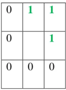
Figure 3: 4 transition (not uniform) left, 2 transitions (uniform), right

The uniformity is can be considered when the measureable key of uniformity is at most 2. For example, in M. Pietikäinen et al book [7], a local binary pattern is called uniform if the pattern of binary is transitioning less than 2 times, “the patterns 00000000 (0 transitions), 01110000 (2

transitions) and11001111 (2 transitions) are uniform whereas the patterns 11001001 (4 transitions) and 01010011 (6 transitions) are not.” The tables above the visual example of LBP’s

uniformity.

2.1.2 CSLBP – Center Symmetric Local Binary Pattern

From Ojala et al. research, the main disadvantage of LBP is that texture in the real life is not always uniform like lungs texture due to the variations of scaling and orientation of visual appearance. Therefore, a lot of additional techniques been applied to modify the original LBP. In this proposal, conventional LBP will be the main technique in doing the analysis. However, the another approach is been used to do the analysis using other LBP variants like center symmetric local binary pattern (CS-LBP), local binary pattern variance (LBPV), completed local binary pattern (CLBP).

Furthermore, not many people try to approach in doing texture analysis of lungs using these 3 LBP variants. The usual parameters that use these 3 variants to do analysis are like facial recognition, etc. Technically, all variants are the same things. The only different is the modification made on its structured [8], [9],[13].

Another approach by Heikkila is CS-LBP, it means only half of the pixel will be considered in doing the analysis. The derivative or equation shown below,

0 1 1 0 1 0 0 0 1 1 0 1 0 0 0 1

(18)

Chapter 2: Literature Review 9 𝑪𝑺 − 𝑳𝑩𝑷(𝒙, 𝒚) = ∑ 𝒔 (𝒏𝒊 + (𝑵 𝟐)) 𝟐𝒊 (𝑵_𝟐)−𝟏 𝒊=𝟎 ______ (9) 𝒔(𝒙) = { 𝟏, 𝒙 > 𝑻 𝟎, 𝒐𝒕𝒉𝒆𝒓𝒘𝒊𝒔𝒆 ____ (10)

CS-LBP is actually a combination of 3D histogram deciptor with conventional LBP histogram. It been developed for interest region description. Therefore, the number of LBP become smaller and the histogram level become shorter. The gray value will be considered when the neighborhood is more than it or vice versa.

2.1.3 LBPV – Local Binary Pattern Variance

The LBPV has been proposed by Zhenhou et.al [14], [15] was to improvise the conventional LBP for the texture model. This technique and approach has been proven have tremendous result because of the joint distribution of LBP and VAR. Quantization is needed for the variation of the images at the pixel and the radius. The purpose of the LBPV is to overcome the limitation of the process of quantization. Due to the different contrast of the images, the variation of the LBP were increased. Therefore, the similarity of specific images will be effected because of the contrast. The equation below shows how rotation invariant measures works for level of contrast of images. The VARP, R will be adjusted for the histogram of LBP to take effect.

2.1.4 CLBP – Completed Local Binary Pattern

The CLBP is the upgraded version of conventional LBP, the texture is still same in a box with 3 x 3 partition. Each of the small box will represented in its own labelled. For example 0, 0 1, 0 2,0 … etc.

From the theory of LBP given by Pietikäinen, the value can be calculated using LBP formula. As 1, 1 pixel is the center, its own value will be compared with the neighbor’s value. If the neighbor’s value is less than the center, it will indicate 0.When the value is greater, it will indicate 1. At the right image is the value of each pixel. From the value, the LBP values will be formed. The biggest different is the effect of sign negative and positive. Unlike the conventional LBP, the main steps to get the value is based on the center value whether it is less or more than the neighbor value.

Therefore, more or less the CLBP takes part in 1. Presentation of the center pixel

(19)

10 2. Differentiation of local difference sign magnitude

3. Combination of LBP in form of center pixel, sign and magnitude

2.2 kNN Classifier (k-Nearest Neighbour)

kNN classifier is an algorithm for classifying different pattern. There will be two main task that will be done by kNN classifier which been called regression and classification. For lung texture classification, regression analysis is being used. kNN classifier is being used due to the abstract texture of the database which the distance matrix can’t be used.

For the classifier, k is been set to an integer as the number of training set been used. For example, k=1, when the samples is been loaded to the algorithm, the samples will come out to some values based on what techniques been used to get the values. If the majority of the samples is near to the specific class value, the sample will be represented in that specific class. It is very important to know the kNN classifier because the classifier is very robust and simple to understand. However, depending on the selection of parameters, for this project, the parameter is LBP. The complexity of variation of LBP will be seen the changes of effectiveness of kNN classifier. The theory of kNN classifier is easy to understand and easy to predict the outcomes. This will be main strength of the kNN classifier.

The values of LBP is not very accurate especially when it is related to the unclear images or textures. The values of the LBP alone without any filter and enhancing of histogram might affected the kNN classifier. This matter will be seen in this report in the chapter 4. The kNN classifier is working based on Euclidean distance. The closer the distance to the point, the response of the value will be accurate. To see the illustration how does the kNN works, refer to the figure 4.

(20)

11 Figure 4: k-NN classifier representation. The circle is been tested to see whether it belongs to the triangle or the square group. The inner circle indicting the k = 3, where the outer circle k = 5. The different k will give a different results in classification. The circle belongs to square group since the square is majority in that circle. While the inner circle shows the vice versa result.

When there are several sets of training images, like X and Y where X is a set of data from sample database and Y is a set of data from training database.

𝑿 = (𝑿𝟏, 𝑿𝟐, 𝑿𝟑, … , 𝑿𝒏)

𝒀 = (𝒀_𝟏, 𝒀_𝟐, 𝒀_𝟑, … , 𝒀_𝒏)

To see the distance the X and Y values will be represented in the following equation.

𝑫(𝑿, 𝒀) = √∑(𝒙_𝒊, 𝒚_𝒊)𝟐 𝒏

𝒊=𝟏

(21)

Chapter 3: Methodology

12

CHAPTER 3 METHODOLOGY

3 Methodology / Project Work 3.1 Lung Classification

To make it clearer what is the LBP is all about, refer to the image below. According to the Lukas Apalovic in his work of summarization of LBP, first there must be a texture and texture classes. The desired texture will be assigned in the respective texture classes. Therefore, there must be some representation or model for the texture. The model is LBP. By converting the bitmap image to the gray level image in this case, each pixel of the image will have its own pixel. Based on Apalovic explanation, from each pixel there will be LBP value.

(left) the pixel from the ROIs of an

image/texture

(center) the representation of the pixel

(right) the pixel value

Figure 5: The representation of LBP

From the left, the ROI will be represented in a box with 3 x 3 partition. Each of the small box will represented in its own labelled. Like 0, 0 1, 0 2,0 … etc. as been shown above (center). From the theory of LBP given by Pietikäinen, the value can be calculated using LBP formula. As 1,1 pixel is the center, its own value will be compared with the neighbor’s value. If the neighbor’s value is less than the center, it will indicate 0.When the value is greater, it will indicate 1. At the right image is the value of each pixel. From the value, the LBP value will be formed.

(22)

Chapter 3: Methodology 13 218 < 157 … 0 218 < 178 … 0 218 < 220 … 1 218 < 255 … 1 218 < 255 … 1 218 < 219 … 1 218 < 215 … 0 218 < 219 … 1

The binary value can be retrieved based on the comparison value. 001111012 = 6110. 61 is the

decimal value inside the LBP histogram. The value been stored each of it until the histogram is complete.

From the image below, the histogram will completed depends on the mapping type [10],[11]. Currently for the project, 3 types of mapping have been done, rotation invariant LBP, uniform LBP and uniform rotation invariant LBP.

Figure 6: The image of histogram (LBP model)

There are 36 unique LBPs for image with 256 gray levels. The texture model can be represented in 36 dimensional point in 36 dimensional space.

For the texture classes, there is a classifier to classify the texture based on the class where it come from. The classifier that had been proposed by Apalovic is k-NN (nearest neighbor). This algorithm is widely been used in classification and regression [5].

k-NN algorithm is very simple. However, small values of k will affect the noise on classification. Therefore, the data were based on the value of k.

(23)

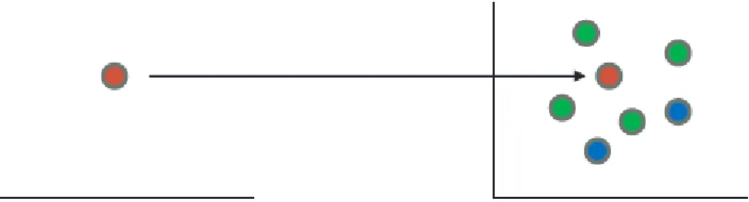
14 Figure 7: k-NN classifier

The red point is the point of interest. In this case, the red point is the set point. The green dots shows more interest towards the red point. Therefore, the red point is the neighbor of green class. This analogy is the most basic in understanding the k-NN classifier. For this project, the representation of matrix form will be used in order to undergo the classification process using k-NN classifier.

Figure 8: Flow of LBP process

From the Figure 8, the flow of LBP process can be summarized:- 1. Reading the image.

2. Separate it block by block (e.g. 3 x 3) 3. The difference of the pixel/gray value gp - gc

(24)

15 5. The magnitude to put in the LBP equation

6. Value of the LBP will be interpret in the histogram equation

From Sorensen et al. [7], it seems like texture analysis of lungs can be analyzed using LBP. However, there are some modifications need to be done [6]. Data of this project been used same like Sorensen et al. in his website. CT scanning was performed using General Electric (GE) equipment (LightSpeed QX/i; GE Medical Systems, Milwaukee, WI, USA) with four detector rows and using the following parameters: in-plane resolution 0.78 x 0.78 mm, slice thickness 1.25 mm, tube voltage 140 kV, and tube current 200 mAs. The slices were reconstructed using a high-spatial-resolution (bone) algorithm. 9 never-smokers, 10 smokers, and 20 smokers with COP been used as the database.

A0024_middle A0024_bottom A0024_top

(a) (b) (c)

Figure 9:- Lung CT scan. From left is the image of CT scan from the middle view (a). The center image is the CT scan of lung from bottom (b) and the most right is the top view (c). These 3 images have different representation to detect the unhealthy tissues.

(25)

16

3.2 Cycle of Experiment

There will several parameters that can be manipulated in this project. First, the database. The database can be most important part in this experiment. The lung database, it’s very hard to get the same output with other database like the face, textile, woods and etc. The size of the image that been retrieved from the database also plays a big role. Larger size of the image may give a different outcome or vice versa. The images of database somehow need to be processed before it can be used in a certain software. In this experiment, MATLAB software been used since the process of LBP is involving feature matrix. Secondly, the main parameters is LBPs techniques. We are using different techniques in order to see the reliability of the techniques. The kNN classifier can be modified to have larger radius of neighbour since the k value can be varies from 1 until infinite.

(26)

Chapter 4: Results & Discussion

17

CHAPTER 4 RESULTS & DISCUSSION

4 Results & Discussion

In this chapter, we present the performance analysis of four types of LBP, namely, conventional Local Binary Pattern (LBP), Center Symmetric Local Binary Pattern (CS-LBP), Completed Local Binary Pattern (CLBP) and Local Binary Pattern Variance (LBPV). The metric used to evaluate the performance is kNN classifier. In section 5.1 show the results of the performance based on LBP. Performance based on CLBP is discussed in section 5.2. While the remaining two techniques will be discussed in section 5.3 and 5.4 respectively. The experiments were run using emphysema image database. Separation of the images been made based on the type of disease at the lung tissues. In order to test the performance of LBP and its derivatives, the experiments conducted by doing the analysis of the images by alienated the lung tissues of the specific subjects with other lung tissues. This experiment is been done by being list in a table to see whether the image is being guess correctly or not. Both databases are set to 256x256. This is to ensure the comparison between the training images and testing image is the same. All experiments were carried out in 64-bit Operating System, x64-based processor on Windows 8 operating system which has 8GB RAM and Intel® Core ™ i7-4510U @ 2.00GHz. MATLAB Version is R2012b.

The tissues images been evaluated based on recognition rate of accuracy by having the total number of correct detection divided by the total number of sample testing images.

𝑨𝒄𝒄𝒖𝒓𝒂𝒄𝒚 (𝒄𝒐𝒓𝒓𝒆𝒄𝒕) =𝑵𝒖𝒎𝒃𝒆𝒓 𝒐𝒇 𝒄𝒐𝒓𝒓𝒆𝒄𝒕 𝒊𝒎𝒂𝒈𝒆𝒔

(27)

18 There will be 109 patches of the lung tissues been used. The 1st patches until 59th is been labelled as the normal tissue (NT). The remaining 50 patches been labelled as unhealthy tissues which is the centrilobular emphysema (CLE). So far, only 4 techniques been used for this experiment which is LBP (local binary pattern), CLBP (completed local binary pattern), Center Symmetric Local Binary Pattern (CS-LBP) and Local Binary Pattern Variance (LBPV). Surprisingly, there will be unexpected results regarding of the techniques. The experiment is still in developing mode whether to decide to use lump sum patches or specific subject been used for the sample texture features or patches. From the 109 patches, we has divided the patches accordingly. Some sample of normal, centrilobular, and paraseptal emphysema patches are given in Table 1.

(28)

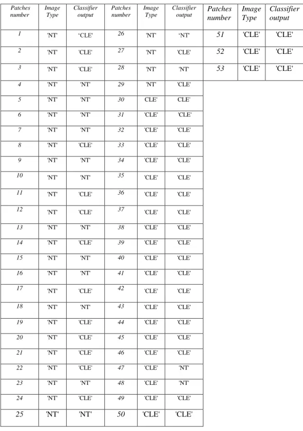
19 Table 1:- List of patches for the database

Normal Tissue Centrilobular Emphysema Paraseptal Emphysema

Patch1 Patch60 Patch110

Patch2 _Patch61 _Patch111

Patch3 Patch62

Patch112

Patch4 Patch63 Patch113

The 1st patches until 30th patches been used as the training database and 31st patches until 59th patches been used as the sample database. Same goes to CLE patches. The 60th patches until 85th patches been used as the training database while 86th patches until 109th patches been used as the sample database.

(29)

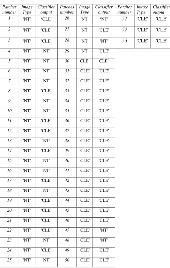
20 In this experiment, classification of emphysema is tested using LBP. The result of the classifier is presented in Table 2. Result in Table 2 shows that 35 images are correctly classified whereas 18 are misclassified. In other word, the LBP gives accuracy of 66.03% and

misclassification rate of 33.97%. The percentage of the match texture is still low because the ratio of the LBP should be more than 80% to show the effectiveness of the LBP.

Table 2 shows the result of emphysema classification of 53 test images using LBP. Left column is the number of patches. The number has been follow exactly like been provided. The middle column is the actual or the correct labelled of the patches. The most right column indicate the output of the patches. The result can be seen whether it’s matched or unmatched by comparing the middle column and the most right column. Some calculation has been made to see and determine the effectiveness of the LBP. The calculation made based on the equation (12).

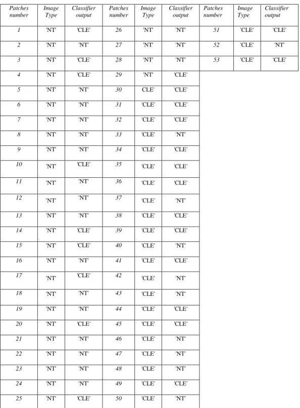
Surprisingly the analysis of the CLBP have the same output with the conventional of normal LBP. The purpose CLBP is to increase the accuracy of the conventional LBP. However, after doing the test. The outcome is same with the conventional LBP. Therefore, we conclude that some extra measures must be taken to overcome the problem. For example, the mapping of the images. By having the same result with the LBP, the accuracy of the correct images is same equal to 66.03%. After some observation been made, the histogram of CLBP somehow is same with the LBP. Therefore, the outcome or the results can be expected same, even the value of the both LBP is plays a big role.

The accuracy of the LBPV technique is 62.26% and the unmatched percentage is 37.74%. Total of correct images are 33. This data can be seen in Table 4. The accuracy of the LBPV is slightly lower compared to the CLBP and the LBP. The accuracy somehow related to the contrast of the images. Since the contrast of the images of CT scan are almost same for all patches inside the database.

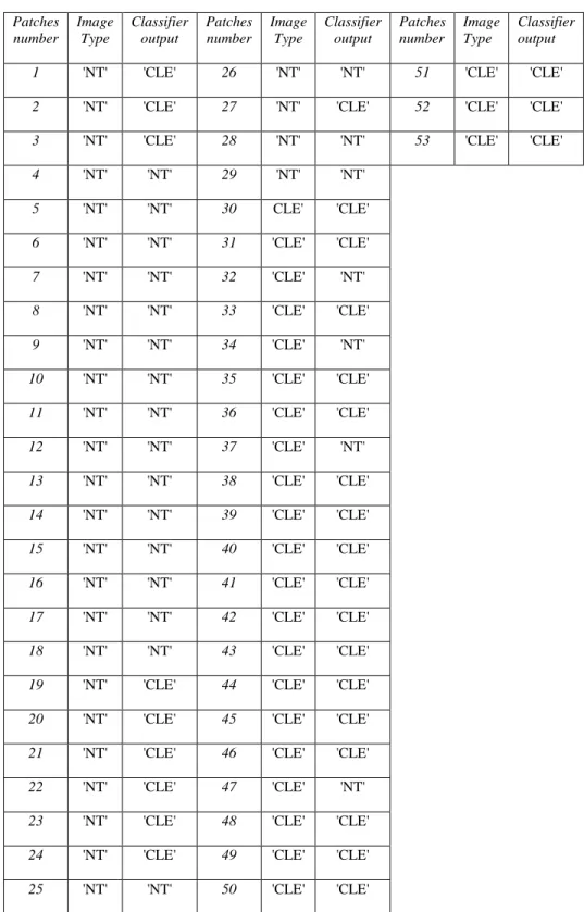
CSLBP shows the highest accuracy amongst the techniques. By referring to the Table 5, 39 images has been correctly match. The percentage of the CSLBP is 73.58% and the unmatched percentage is 26.42%. Based on the theory of CSLBP, half of the pixel has been focused on the patches. Since the reduction of the patches has been made, the outer layer of the lung tissues or patches might been ignored.

(30)

21

Local Binary Pattern (LBP)

Table 2: List of the results of LBP with emphysema database

Patches number Image Type Classifier output Patches number Image Type Classifier

output Patches _number Image _Type Classifier _output

1 _'NT' _‘CLE' 26 _'NT' _‘NT' ₅₁ _'CLE' _'CLE'

2 _'NT' _'CLE' 27 _'NT' _'CLE' ₅₂ _'CLE' _'CLE'

3 _'NT' _'CLE' 28 _'NT' _'NT' ₅₃ _'CLE' _'CLE'

4 'NT' 'NT' 29 'NT' 'CLE'

5 'NT' 'NT' 30 CLE' CLE'

6 'NT' 'NT' 31 'CLE' 'CLE'

7 'NT' 'NT' 32 'CLE' 'CLE'

8 'NT' 'CLE' 33 'CLE' 'CLE'

9 'NT' 'NT' 34 'CLE' 'CLE'

10 _'NT' _'NT' 35 _'CLE' _'CLE'

11 _'NT' _'CLE' 36 _'CLE' _'CLE'

12 _'NT' _'CLE' 37 _'CLE' _'CLE'

13 'NT' 'NT' 38 'CLE' 'CLE'

14 'NT' 'CLE' 39 'CLE' 'CLE'

15 'NT' 'NT' 40 'CLE' 'CLE'

16 'NT' 'NT' 41 'CLE' 'CLE'

17 _'NT' _'CLE' 42 _'CLE' _'CLE'

18 'NT' 'NT' 43 'CLE' 'CLE'

19 'NT' 'CLE' 44 'CLE' 'CLE'

20 'NT' 'CLE' 45 'CLE' 'CLE'

21 'NT' 'CLE' 46 'CLE' 'CLE'

22 'NT' 'CLE' 47 'CLE' 'NT'

23 'NT' 'NT' 48 'CLE' 'NT'

24 'NT' 'CLE' 49 'CLE' 'CLE'

(31)

22

Completed Local Binary Pattern (CLBP)

Table 3:- List of the results of CLBP with emphysema database Patches number Image Type Classifier output Patches number Image Type Classifier output Patches number Image Type Classifier output 1 _'NT' _‘CLE' 26 _'NT' _‘NT' ₅₁ _'CLE' _'CLE' 2 _'NT' _'CLE' 27 _'NT' _'CLE' ₅₂ _'CLE' _'CLE' 3 _'NT' _'CLE' 28 _'NT' _'NT' ₅₃ _'CLE' _'CLE' 4 'NT' 'NT' 29 'NT' 'CLE'

5 'NT' 'NT' 30 CLE' CLE'

6 'NT' 'NT' 31 'CLE' 'CLE'

7 'NT' 'NT' 32 'CLE' 'CLE'

8 'NT' 'CLE' 33 'CLE' 'CLE'

9 'NT' 'NT' 34 'CLE' 'CLE'

10 'NT' 'NT' 35 'CLE' 'CLE'

11 'NT' 'CLE' 36 'CLE' 'CLE'

12 'NT' 'CLE' 37 'CLE' 'CLE'

13 'NT' 'NT' 38 'CLE' 'CLE'

14 'NT' 'CLE' 39 'CLE' 'CLE'

15 'NT' 'NT' 40 'CLE' 'CLE'

16 'NT' 'NT' 41 'CLE' 'CLE'

17 'NT' 'CLE' 42 'CLE' 'CLE'

18 'NT' 'NT' 43 'CLE' 'CLE'

19 'NT' 'CLE' 44 'CLE' 'CLE'

20 'NT' 'CLE' 45 'CLE' 'CLE'

21 'NT' 'CLE' 46 'CLE' 'CLE'

22 'NT' 'CLE' 47 'CLE' 'NT'

23 'NT' 'NT' 48 'CLE' 'NT'

24 'NT' 'CLE' 49 'CLE' 'CLE'

(32)

23

Local Binary Pattern Variance (LBPV)

Table 4:- List of the results of LBPV with emphysema database

Patches number Image Type Classifier output Patches number Image Type Classifier output Patches number Image Type Classifier output

1 'NT' 'CLE' 26 'NT' 'NT' 51 'CLE' 'CLE'

2 'NT' 'NT' 27 'NT' 'NT' 52 'CLE' 'NT'

3 'NT' 'CLE' 28 'NT' 'NT' 53 'CLE' 'CLE'

4 'NT' 'CLE' 29 'NT' 'CLE' 5 'NT' 'NT' 30 CLE' 'CLE' 6 'NT' 'NT' 31 'CLE' 'CLE' 7 'NT' 'NT' 32 'CLE' 'CLE' 8 'NT' 'NT' 33 'CLE' 'NT' 9 'NT' 'NT' 34 'CLE' 'CLE'

10 _'NT' 'CLE' 35 _'CLE' _'CLE'

11 'NT' 'NT' 36 'CLE' 'CLE'

12 _'NT' 'NT' 37 _'CLE' _'NT'

13 'NT' 'NT' 38 'CLE' 'CLE'

14 'NT' 'CLE' 39 'CLE' 'CLE'

15 'NT' 'CLE' 40 'CLE' 'NT'

16 'NT' 'NT' 41 'CLE' 'CLE'

17 _'NT' 'CLE' 42 _'CLE' _'NT'

18 'NT' 'NT' 43 'CLE' 'NT'

19 'NT' 'NT' 44 'CLE' 'CLE'

20 'NT' 'CLE' 45 'CLE' 'CLE'

21 'NT' 'NT' 46 'CLE' 'NT'

22 'NT' 'NT' 47 'CLE' 'NT'

23 'NT' 'NT' 48 'CLE' 'NT'

24 'NT' 'NT' 49 'CLE' 'CLE'

(33)

24

Center Symmetric Local Binary Pattern (CSLBP)

Table 5:- List of the results of CSLBP with emphysema database

Patches number Image Type Classifier output Patches number Image Type Classifier output Patches number Image Type Classifier output 1 'NT' 'CLE' 26 'NT' 'NT' 51 'CLE' 'CLE' 2 'NT' 'CLE' 27 'NT' 'CLE' 52 'CLE' 'CLE' 3 'NT' 'CLE' 28 'NT' 'NT' 53 'CLE' 'CLE' 4 'NT' 'NT' 29 'NT' 'NT' 5 'NT' 'NT' 30 CLE' 'CLE' 6 'NT' 'NT' 31 'CLE' 'CLE' 7 'NT' 'NT' 32 'CLE' 'NT' 8 'NT' 'NT' 33 'CLE' 'CLE' 9 'NT' 'NT' 34 'CLE' 'NT' 10 'NT' 'NT' 35 'CLE' 'CLE' 11 'NT' 'NT' 36 'CLE' 'CLE' 12 'NT' 'NT' 37 'CLE' 'NT' 13 'NT' 'NT' 38 'CLE' 'CLE' 14 'NT' 'NT' 39 'CLE' 'CLE' 15 'NT' 'NT' 40 'CLE' 'CLE' 16 'NT' 'NT' 41 'CLE' 'CLE' 17 'NT' 'NT' 42 'CLE' 'CLE' 18 'NT' 'NT' 43 'CLE' 'CLE' 19 'NT' 'CLE' 44 'CLE' 'CLE' 20 'NT' 'CLE' 45 'CLE' 'CLE' 21 'NT' 'CLE' 46 'CLE' 'CLE' 22 'NT' 'CLE' 47 'CLE' 'NT' 23 'NT' 'CLE' 48 'CLE' 'CLE' 24 'NT' 'CLE' 49 'CLE' 'CLE' 25 'NT' 'NT' 50 'CLE' 'CLE'

(34)

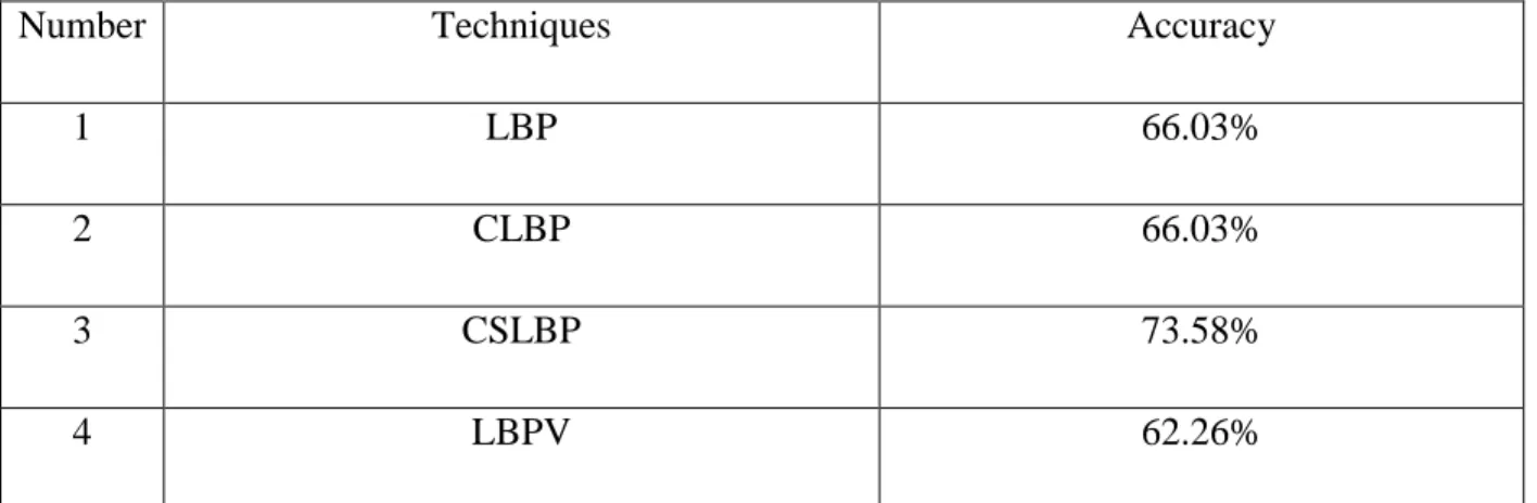
25 Table 6:- Summarization of the LBP techniques.

Number Techniques Accuracy

1 LBP 66.03%

2 CLBP 66.03%

3 CSLBP 73.58%

4 LBPV 62.26%

Table 6 shows the summarization of the accuracy of the emphysema classification. LBPV shows the lowest accuracy and CSLBP shows the highest accuracy. The remaining two techniques show the same result.

(35)

26

CHAPTER 5

CONCLUSION AND FURTHER RESEARCH WORK 5 Conclusion and Further Research Work

5.1 Conclusion

The result of LBP has been shown in this report. The histograms of LBP can be extracted from all patches and been combined to form a matrix. After that, kNN classifier will be used to classify and evaluate the reliability of the LBP. The experiment or project have to be sorted and use the correct database. The hypothesis for this project is, the local binary pattern can be used for lung texture analysis.

In conclusion, based on the result from the experiment, LBP still cannot be concluded as the best method for lung texture. This is because there are still a few variants that can be used for lung texture analysis technique in future research and some modification has to be made on the LBP.

5.2 Further research work on LBP

In this work, we have presented the performance studies of LBPs-based emphysema classification of lung CT images. The four evaluated LBPs are conventional LBP, CS-LBP, LBPV and CLBP. These LBPs are used to extract the feature of the CT images prior to being input to a kNN classifier. Result generated in this work shows the best classification accuracy is obtained when using the CSLBP. However, the value is only 73.58% which is considered as not acceptable for diagnosis of emphysema. The accuracy can be improved by using Gabor wavelet as additional feature extraction technique. The hybrid of Gabor-LBP based technique is expected to improve the classification accuracy since Gabor wavelet gives the global image feature whereas the LBP gives the local image feature. This hypothesis, however, remain to be investigated.

(36)

27

6 References

[1] Mannino, D. M., et al. (2006). "Global Initiative on Obstructive Lung Disease (GOLD) classification of lung disease and mortality: findings from the Atherosclerosis Risk in Communities (ARIC) study." Respiratory Medicine 100(1): 115-122.

[2] Borge, C. R., et al. (2014). "Illness perception in people with chronic obstructive pulmonary disease." Scandinavian Journal of Psychology 55(5): 456-463.

[3] Chen, J., et al. (2010). "WLD: a robust local image descriptor." IEEE Trans Pattern Anal Mach Intell 32(9): 1705-1720.

[4] M. Heikkilä, et al. (2009). "Computer Vision Using Local Binary Patterns." 40: 400-450. [5] Altman, N. S. (1992). "An introduction to kernel and nearest-neighbor nonparametric regression". The American Statistician46 (3): 175–185.

[6] Everitt, B. S., Landau, S., Leese, M. and Stahl, D. (2011) Miscellaneous Clustering Methods, in Cluster Analysis, 5th Edition, John Wiley & Sons, Ltd, Chichester, UK.

[7] Sorensen, L., et al. (2008). "Texture classification in lung CT using local binary patterns." Med Image Comput Comput Assist Interv 11(Pt 1): 934-941.

[8] Sorensen, L., et al. (2010). "Quantitative analysis of pulmonary emphysema using local binary patterns." IEEE Trans Med Imaging 29(2): 559-569.

[9] Zulueta-Coarasa, T., et al. (2013). "Emphysema classification based on embedded probabilistic PCA." Conf Proc IEEE Eng Med Biol Soc 2013: 3969-3972.

[10] M. Heikkilä, M. Pietikäinen, and C. Schmid, "Description of interest regions with local binary patterns," Pattern Recognition, vol. 42, pp. 425-436, 3// 2009.

[11] G. Donato, M. S. Bartlett, J. C. Hager, P. Ekman, and T. J. Sejnowski, "Classifying facial actions," Pattern Analysis and Machine Intelligence, IEEE Transactions on, vol. 21, pp. 974-989, 1999. [12] T. Ahonen, A. Hadid, and M. Pietikäinen, "Face Recognition with Local Binary Patterns," in

Computer Vision - ECCV 2004. vol. 3021, T. Pajdla and J. Matas, Eds., ed: Springer Berlin Heidelberg, 2004, pp. 469-481.

[13] M. Heikkilä, M. Pietikäinen, and C. Schmid, "Description of interest regions with local binary patterns," Pattern Recognition, vol. 42, pp. 425-436, 3// 2009.

[14] Z. Guo, L. Zhang, and D. Zhang, "Rotation invariant texture classification using LBP variance (LBPV) with global matching," Pattern Recognition, vol. 43, pp. 706- 719, 3// 2010.

[15] G. Zhenhua, D. Zhang, and D. Zhang, "A Completed Modeling of Local Binary Pattern Operator for Texture Classification," Image Processing, IEEE Transactions on, vol. 19, pp. 1657-1663, 2010.

(37)

28

7 Appendices Coding for LBP

clear all;close all;clc

fet1=zeros(1,59);

for images=1:30

str = strcat(int2str(images),'.mat'); %% In this case image files should be in same Folder eval('load(str);'); % figure(images); imshow(I,[]) mapping=getmapping(8,'riu2'); H=lbp(I,1,8,mapping); %%%LBPV(I,R,P,MAPPING) fet1=cat(1,fet1,H); end fet2=zeros(1,59); for images=60:85

str = strcat(int2str(images),'.mat'); %% In this case image files should be in same Folder eval('load(str);'); % figure(images); imshow(I,[]) mapping=getmapping(8,'riu2'); H=lbp(I,1,8,mapping); fet2=cat(1,fet2,H); end B = [fet1(2:31,:); fet2(2:27,:)]; G = {'NT';'NT';'NT';'NT';'NT';'NT';'NT';'NT';'NT';'NT';'NT';'NT';'NT';'NT';'NT';

(38)

29

'NT';'NT';'NT';'NT';'NT';'NT';'NT';'NT';'NT';'NT';'NT';'NT';'NT';'NT';'NT';' CLE';'CLE';'CLE';'CLE';'CLE';'CLE';'CLE';'CLE';'CLE';'CLE';'CLE';'CLE';'CLE'

;'CLE';'CLE';'CLE';'CLE';'CLE';'CLE';'CLE';'CLE';'CLE';'CLE';'CLE';'CLE';'CL E'}; %%%

%NT_sample

fet3=zeros(1,59);

for images=31:59

str = strcat(int2str(images),'.mat'); %% In this case image files should be in same Folder eval('load(str);'); % figure(images); imshow(I,[]) mapping=getmapping(8,'riu2'); H=lbp(I,1,8,mapping); fet3=cat(1,fet3,H); end %CLE_sample fet4=zeros(1,59); for images=86:109

str = strcat(int2str(images),'.mat'); %% In this case image files should be in same Folder eval('load(str);'); % figure(images); imshow(I,[]) mapping=getmapping(8,'riu2'); H=lbp(I,1,8,mapping); fet4=cat(1,fet4,H); end

(39)

30 A = [fet3(2:30,:); fet4(2:25,:)];

%A, sample (the one been grouped__the result) %B, training (must same with G the total) class = knnclassify(A, B, G);

Coding for CLBP

clear all;close all;clc fet1=zeros(1,59);

for images=1:30

str = strcat(int2str(images),'.mat'); %% In this case image files should be in same Folder eval('load(str);'); % figure(images); imshow(I,[]) mapping=getmapping(8,'riu2'); H=clbp(I,1,8,mapping); %%%LBPV(I,R,P,MAPPING) fet1=cat(1,fet1,H); end fet2=zeros(1,59); for images=60:85

str = strcat(int2str(images),'.mat'); %% In this case image files should be in same Folder

eval('load(str);');

% figure(images); imshow(I,[]) mapping=getmapping(8,'riu2');

(40)

31 fet2=cat(1,fet2,H); end B = [fet1(2:31,:); fet2(2:27,:)]; G = {'NT';'NT';'NT';'NT';'NT';'NT';'NT';'NT';'NT';'NT';'NT';'NT';'NT';'NT';'NT'; 'NT';'NT';'NT';'NT';'NT';'NT';'NT';'NT';'NT';'NT';'NT';'NT';'NT';'NT';'NT';' CLE';'CLE';'CLE';'CLE';'CLE';'CLE';'CLE';'CLE';'CLE';'CLE';'CLE';'CLE';'CLE'

%NT_sample

fet3=zeros(1,59);

for images=31:59

str = strcat(int2str(images),'.mat'); %% In this case image files should be in same Folder eval('load(str);'); % figure(images); imshow(I,[]) mapping=getmapping(8,'riu2'); H=clbp(I,1,8,mapping); fet3=cat(1,fet3,H); end %CLE_sample fet4=zeros(1,59); for images=86:109

eval('load(str);');

(41)

32 mapping=getmapping(8,'riu2'); H=clbp(I,1,8,mapping); fet4=cat(1,fet4,H); end A = [fet3(2:30,:); fet4(2:25,:)];

Coding for CSLBP

clear all;close all;clc

fet1=zeros(1,16);

for images=1:30

str = strcat(int2str(images),'.mat'); %% In this case image files should be in same Folder eval('load(str);'); % figure(images); imshow(I,[]) mapping=getmapping(8,'u2'); H=CSLBP(I)'; %%%LBPV(I,R,P,MAPPING) fet1=cat(1,fet1,H); end fet2=zeros(1,16); for images=60:85

(42)

33 str = strcat(int2str(images),'.mat'); %% In this case image files should be in same Folder eval('load(str);'); % figure(images); imshow(I,[]) mapping=getmapping(8,'u2'); H=CSLBP(I)'; fet2=cat(1,fet2,H); end B = [fet1(2:31,:); fet2(2:27,:)]; G = {'NT';'NT';'NT';'NT';'NT';'NT';'NT';'NT';'NT';'NT';'NT';'NT';'NT';'NT';'NT'; 'NT';'NT';'NT';'NT';'NT';'NT';'NT';'NT';'NT';'NT';'NT';'NT';'NT';'NT';'NT';' CLE';'CLE';'CLE';'CLE';'CLE';'CLE';'CLE';'CLE';'CLE';'CLE';'CLE';'CLE';'CLE'

%NT_sample

fet3=zeros(1,16);

for images=31:59

str = strcat(int2str(images),'.mat'); %% In this case image files should be in same Folder eval('load(str);'); % figure(images); imshow(I,[]) mapping=getmapping(8,'u2'); H=CSLBP(I)'; fet3=cat(1,fet3,H); end %CLE_sample

(43)

34 fet4=zeros(1,16);

for images=86:109

str = strcat(int2str(images),'.mat'); %% In this case image files should be in same Folder eval('load(str);'); % figure(images); imshow(I,[]) mapping=getmapping(8,'u2'); H=CSLBP(I)'; fet4=cat(1,fet4,H); end A = [fet3(2:30,:); fet4(2:25,:)];

Coding for LBPV

clear all;close all;clc fet1=zeros(1,10);

for images=1:30

str = strcat(int2str(images),'.mat'); %% In this case image files should be in same Folder eval('load(str);'); % figure(images); imshow(I,[]) mapping=getmapping(8,'riu2'); H=LBPV(I,1,8,mapping); %%%LBPV(I,R,P,MAPPING)

(44)

35 fet1=cat(1,fet1,H);

end

fet2=zeros(1,10);

for images=60:85

str = strcat(int2str(images),'.mat'); %% In this case image files should be in same Folder eval('load(str);'); % figure(images); imshow(I,[]) mapping=getmapping(8,'riu2'); H=LBPV(I,1,8,mapping); fet2=cat(1,fet2,H); end B = [fet1(2:31,:); fet2(2:27,:)]; G = {'NT';'NT';'NT';'NT';'NT';'NT';'NT';'NT';'NT';'NT';'NT';'NT';'NT';'NT';'NT'; 'NT';'NT';'NT';'NT';'NT';'NT';'NT';'NT';'NT';'NT';'NT';'NT';'NT';'NT';'NT';' CLE';'CLE';'CLE';'CLE';'CLE';'CLE';'CLE';'CLE';'CLE';'CLE';'CLE';'CLE';'CLE'

%NT_sample

fet3=zeros(1,10);

for images=31:59

eval('load(str);');

% figure(images); imshow(I,[]) mapping=getmapping(8,'riu2');

(45)

36 H=LBPV(I,1,8,mapping); fet3=cat(1,fet3,H); end %CLE_sample fet4=zeros(1,10); for images=86:109

str = strcat(int2str(images),'.mat'); %% In this case image files should be in same Folder eval('load(str);'); % figure(images); imshow(I,[]) mapping=getmapping(8,'riu2'); H=LBPV(I,1,8,mapping); fet4=cat(1,fet4,H); end A = [fet3(2:30,:); fet4(2:25,:)];