ISSN: 2088-8708, DOI: 10.11591/ijece.v10i3.pp2651-2658 2651
Predictive geospatial analytics using principal component
regression
Kyi Lai Lai Khine1, Thi Thi Soe Nyunt2
1Cloud Computing Lab, University of Computer Studies, Myanmar 2Faculty of Computer Science, University of Computer Studies, Myanmar
Article Info ABSTRACT
Article history: Received Mar 31, 2019 Revised Nov 3, 2019 Accepted Nov 26, 2019
Nowadays, exponential growth in geospatial or spatial data all over the globe, geospatial data analytics is absolutely deserved to pay attention in manipulating voluminous amount of geodata in various forms increasing with high velocity. In addition, dimensionality reduction has been playing a key role in high-dimensional big data sets including spatial data sets which are continuously growing not only in observations but also in features or dimensions. In this paper, predictive analytics on geospatial big data using Principal Component Regression (PCR), traditional Multiple Linear Regression (MLR) model improved with Principal Component Analysis (PCA), is implemented on distributed, parallel big data processing platform. The main objective of the system is to improve the predictive power of MLR model combined with PCA which reduces insignificant and irrelevant variables or dimensions of that model. Moreover, it is contributed to present how data mining and machine learning approaches can be efficiently utilized in predictive geospatial data analytics. For experimentation, OpenStreetMap (OSM) data is applied to develop a one-way road prediction for city Yangon, Myanmar. Experimental results show that hybrid approach of PCA and MLR can be efficiently utilized not only in road prediction using OSM data but also in improvement of traditional MLR model.
Keywords:
Dimensionality reduction Geospatial data analytics Multiple linear regression Open street map
Principal component analysis
Copyright © 2020 Institute of Advanced Engineering and Science. All rights reserved. Corresponding Author:
Kyi Lai Lai Khine, Cloud Computing Lab,
University of Computer Studies,
No. 4, Main Road, Shwe Pyi thar Township, Yangon, Myanmar. Email: [email protected]
1. INTRODUCTION
Big data can be described as large volumes of data in complex structures increasing with high velocity which requires advanced technologies, methods and algorithms to acquire, process and store efficiently [1]. Nowadays, it can be estimated that data about 2.5 quintillion bytes approximately is being generated every day and a large portion of data among them is location-aware. Therefore, it can be assumed that big data where a significant portion of it is typically geospatial data or spatial data. Geospatial or spatial big data is deserved to pay attention in analyzing large-scale spatial data sets which exceed traditional computing systems [2]. Increasing enormous amount of geospatial data, the capability of high-performance computing has been an essential requirement to fully utilize huge collection of geospatial big data with high-velocity in demanding applications. The distributed and parallel computing on a cluster of commodity computers for big data analysis such as Hadoop and Spark have become popular in current time. It can provide geospatial big data analytics easily implemented on big data platforms [3, 4]. With the rapid development in technologies, increasing in computational power and decreasing in data collection cost and processing, dimensions of data sets are continuously growing in size. In these data sets, the dimensions or feature variables “n” can be as high as in size or much higher than the observation size “m”. Among
thousands of dimensions or feature variables, only a small number or subset of them are possible to extract value or insight in data analysis. Therefore, it makes a critical situation to identify correctly and to reduce efficiently them. And, finding significant and relevant features in data sets will fulfill valuable insights to support better decision making. Dimensionality reduction has been playing a key role in high-dimensional large-scale data nature. In addition, the most frequent issue of data mining and machine learning for regression model is that how to predict the outcome of a dependent variable when there are a large number of independent variables in the model. With the advanced technologies and modern algorithms for regression model, it is a difficult situation to handle all variables at once for the model. Chaman Lal, Sabharwal and Anjum [5] presented an adaptive hybrid approach by applying PCA to traditional regression algorithms to reduce the dimensionality of a data set as identifying pattern in data of high dimension can be very hard in data analysis applications. The central idea of using PCA is to fulfill an advantage of lossless data reduction in two diverse areas such as qualitative spatial reasoning (QSR) and health informatics. They also expressed that applying PCA with hybrid approach in two areas, QSR and health informatics is not only a procedure for identifying a small number of “principal components” for reduced dimensions but also a procedure for improving traditional regression algorithms. Improving the predictive power of traditional multiple linear regression model using PCA is studied by Ahmad Zia UI-Saufie, Ahmad Shukri Yahya and Nor Ramli [6] to predict PM10 concentration for next day. Application of PCA in regression models is intended to avoid multicollinearity problem and to ensure that principal components selected have maximum variance. According to experimental studies, they proved that the principal components as input to regression process offer a more accurate result than original data input to regression process because of reduced number of inputs. Therefore, applying PCA based regression models can be considered as more efficient and decreased complexity models. In current time, huge amount of geospatial data can be generated from hundreds of millions of mobile phones, sensors, satellites and other resources [7]. OpenStreetMap (OSM) is an open source data resource for geographic information all over the world. The size of OSM data sets increases significantly in every year because it is a huge collection of geospatial information. Stefan Funke, Robin Schirrmeister and Sabine Storandt [8] introduced that how to apply methods in detection of gaps in the road network automatically and then discovery of missing street names by using OSM road network data. They showed that data mining and machine learning methods are very useful to detect missing road network data in OSM. Growing rapidly in volume and popularity of geospatial data, Geographical Information System (GIS) applications are demanding to data mining and machine learning approaches integrated with spatial big data. Hemlata Goyal, Chilka Sharma and Nisheeth Joshi presented issues, challenges, tools and algorithms for spatial data mining collaborated with big spatial data [2].
2. GEOSPATIAL OR SPATIAL BIG DATA
Geographical location-aware data which is usually stored as coordinates and topology for mapping can be referred to as geospatial or spatial data [9]. Geospatial big data cannot be assumed as new issue or problem in data analytics era. Due to not only exponential increase in data production but also in data production rate (velocity). In EOSDIS, 4TB of remote sensing data archives are growing in every day. This data flow means more than 630 million data files, nearly 20 TB can be delivered to users all over the world. The observation data of NASA in each unit time can be collected from approximately 100 active missions which would be about 1.73GB. High performance computing or cloud computing platforms are absolutely required in analyzing large-scale geospatially enabled contents. By analyzing geospatial data, we can make innovative activities in our daily life and business [10, 11]. In general, we can classify geospatial data into three categories such as raster data, vector data, and graph data. Raster data consists of geoimages taken by digital cameras, satellite etc. and it can be utilized by digital map services, for example, Google Earth. Map data belongs to vector data category which includes points, lines, and polygons, for example, OpenStreetMap.The graph data appears in the form of city maps including roads and landmark. In road networks, an edge can be represented as a segment of road, and a node as an intersection or a landmark. OpenStreetMap (OSM) is an open source data resource for geographic information all over the world. The raw, unstructured large-scale OSM data can be available for developers to create freely to modify the map of the world. It uses a topological data format with four main elements (also known as data primitives): nodes, ways, relations and tags. OSM map data generally represents physical features on the ground, for example, roads or buildings by using tags which describes a geographic attribute showing specific node, way or relation data structures [8]. Many well-known applications and services collaborating with some kinds of geolocation or map-based component using OSM data are as follows: OpenStreetMap-based map for iPhoto for iOS and it has been cited a lot of sources for Apple's custom maps in iOS 6. Interactive data visualization products by Tableau software company has integrated OSM for all their mapping requirements. The professional robot simulator widely used for educational purposes, Webots
applies OSM data to create virtual environment for autonomous vehicle simulations. The large-scale unstructured XML form OSM data can be served as a reality fulfillment of GIS market and spatial world [12, 13].
3. RESEARCH METHOD
3.1. Multiple linear regression (MLR)
Regression analysis, a statistical process, is widely used for prediction and forecasting by estimating relationships between variables. It is not straight forward for large-scale data sets [14]. In this system, multiple linear regression model is applied to predict one-way roads for city Yangon. Multiple Linear Regression (MLR), a statistical model, is intended for estimating the relationship between a dependent variable “Y” and one or more explanatory variables (or independent variables) “X” to obtain the unknown regression model’s parameter “β”. The purpose of minimizing the sum of squares of differences between the predicted values and observed values, estimates for “β” values can be calculated from the regression equation as follow.
Y = β0+β1X1+…………+βnXn (1)
where Y is a dependent variable, X1…...Xn are independent variables and β0 ………βn are coefficients or
parameters of regression model. MLR also specifies how much dependency or connection exist between “Y” and one or more “Xs”. Traditional MLR procedures can be seen in the algorithm 3.1.1.
3.1.1. Algorithm for traditional multiple linear regression Input: m x n data matrix “D”
Output: Predicted “Y”, R2 and RMSE
Steps
1. Define dependent variable “Y” and independent variables “Xs” for matrix Dmxn
2. Find “β” values from the equation (1)
3. Compute predicted “Y” using “β” values and “Xs” 4. Calculate R2 and RMSE for model performance
According to algorithm 3.1.1, there are several input dimensions or independent variables “Xs” for MLR model. Adding all independent variables “Xs” at once to construct a model may be reasonable for small and moderate dimensions in data sets, however, it will be complicated and time-consuming procedure for high-dimensional data nature [15]. In general, several independent variables “Xs” for dependent variable “Y” can be some bias which is very likely to reduce RMSE, a performance indicator of MLR. Therefore, independent variables “Xs” which may affect MLR’s predictive power should be dropped or removed from the model in the analysis. In predictive data analysis, selecting subset of features or dimensions from high-dimensional data sets has become a big issue to improve model’s predictive power because it is a difficult computational problem to deal with very high-dimensions. Moreover, high-dimensional data analysis has been a great attention in big data era. The complexity of big data often makes dimension reduction techniques necessary before conducting statistical inference. The main purpose of dimensionality reduction is to find out how many dimensions can be reduced from all diverse and raw data dimensions. As the number of dimensions of data increases, it becomes more and more difficult to process it. The exponential increasing in the size of data caused by a large number of dimensions in big data make a big problem in data analysis. This is “Curse of Dimensionality” in high-dimensional big data analytics. Principal Component Analysis (PCA), a mathematical procedure, is applied to reduce the dimensionality of data matrix. PCA can often serve as the first processing step in data analysis [15-17]. It may be followed by linear regression, multiple linear regression, cluster analysis, image analysis, and many others.
3.2. Dimensionality reduction using PCA
In current time, dimensionality reduction has been playing a key role in high-dimensional voluminous amount of data. PCA performs dimensionality reduction by extracting the principal components (PCs) of high-dimensional data. In general, data sets can be represented as matrices and vectors with a lot of features. For a matrix, each column refers to a conceptual attribute of all the data. Reducing big original data matrix into smaller one but retaining the same information of original data matrix to gain value or insight from this. Computing PCA of a matrix Y of size N ×D (N rows and D columns), it can be obtained “d” principal components (d ≤ D) that explains the most variance (information) of the data in matrix Y [18-20]. The input for PCA is mainly numerical form. If the data is other form, for example, categorical or logical, it must be converted into numeric first. And then, eigenvalues and eigenvectors are computed to transform original high-dimensional data matrix into lower dimensional one. PCA
decomposition for a data matrix A which is square and symmetric is A = UDUT where U is matrix of eigenvectors and D is diagonal matrix of eigenvalues of A. PCA also arranges eigenvalues by ordering in descending magnitude [21]. In data mining, each observation is a vector with “n” components in a “m x n” data matrix. The first principal component (PC) which is extracted from PCA process will be a maximum amount of variance in the observed data variables. The second principal component or second PC will be uncorrelated with the first PC and the remaining PCs computed from PCA possess the same characteristics [19, 22, 23]. In this system, we would like to prove that PCA which is mostly applied in dimensionality reduction can also effectively reduce insignificant and sometimes, noisy predictors or independent variables of multiple linear regression model. There are a number of reasons why predictor selection becomes an essential role in constructing the optimal regression model. Redundant predictors can hinder the regression analysis while we are trying to explain data in the simplest way and insignificant predictors are also highly potential to increase noises and biases for the model. In addition, a large number of predictors will also cause a problem called “Multicollinearity”. It is a statistical phenomenon of existing a perfect or exact relationship between predictors which will cause incorrectness about the relationship between predictors and outcme variable of that regression model [24]. Therefore, if we apply the model with redundant predictors for prediction purpose, it will be time-consuming and high expensive job indeed. The improved version of MLR combined with PCA can also be seen in the algorithm 3.2.1.
3.2.1. Algorithm for improved multiple linear regression using PCA Input: m x n data matrix “D” (“n” dimensions)
Output: Predicted “Y”, R2 and RMSE
Steps
1. Apply PCA on high-dimensional matrix Dmxn
i. Compute eigenvalues and eigenvectors of Dmxn
ii. Choose top “k” PCs by ranking the eigenvalues from eigenvectors in descending order iii. Construct the matrix Dmxn using “k” eigenvectors into Dmxnk
iv. Reconstruct the matrix Dmxnk into original input matrix form with reduced “nk” dimensions
2. Define dependent variable “Y” and independent variables “Xs” for matrix Dmxnk
3. Find “β” values from the equation (1)
4. Compute predicted “Y” using “β” values and “Xs” 5. Calculate R2 and RMSE for model performance
According to algorithm 3.2.1, it is clearly known that applying PCA procedures before MLR model can offer reduced number of dimensions or variables (“n into nk”) in defining independent variables “Xs” for that model. Therefore, there is no need to utilize all dimensions or independent variables as inputs directly to the model.
3.3. Geospatial OSM data for one-way road prediction
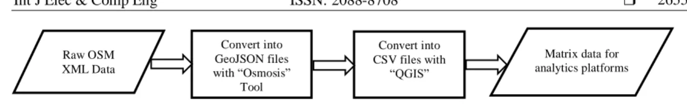
One-way roads and streets are usually used in high volume situations which occur in downtown areas with closely-spaced intersections. In Yangon, the former capital and now business city of Myanmar, roads and streets are often congested and people lose much time stuck in traffic every day. Peak hours are 8:00 to 9:00 in the morning, 14:00 to 16:00 in the evening and after work hours. Sometimes, a ten minutes trip could take as long as 2 hours because of severe traffic situation during peak hours. Although one-way roads and streets can cause some disadvantages such as increased travel distance, wider pedestrian crossings, and driver confusion, it can offer some important advantages such as enhance traffic capacity and increase safety. Not only providing additional lanes and reducing number and severity of crashes by eliminating head-on crashes to be efficient in traffic chead-ontrol operatihead-on and increased safety. The main purpose of implementing this system will predict one-way roads in major business city Yangon using OSM data as a way to facilitate the traffic problems. Moreover, OSM data applying MLR combined with PCA is intended to show that it can fulfill the requirements of predictive geospatial analytics. There is an issue in generating geospatial data and preprocessing for further applying in diverse domains [25]. In general, OSM data exists in the form of data structures such as nodes, ways and relations. It is essential to transform the raw, unstructured OSM XML format data into suitable format compatible with big data analytics platforms such as MapReduce and Spark can be seen in Figure 1. OSM data (OSM XML) is firstly converted into GeoJSON files by using Osmosis, a command-line tool for manipulating raw state OSM data. It can be applied to process large-scale data files. GeoJSON, representing geodata as JSON, is intended to apply in encoding of various geographic data structures. For geospatial data analysis in big data platforms, geodata in JSON format, GeoJSON files are then converted into CSV files by using QGIS (Quantum GIS) which allows users to view, edit and analyse spatial information.
Figure 1. OSM data pre-processing steps
4. RESULTS AND ANALYSIS
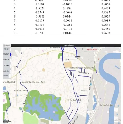
To implement one-way road prediction using OSM data, experiments are performed on Amazon Elastic Compute Cloud (Amazon EC2), a web service, which provides resizable computing capacity and EMR (Elastic MapReduce) for creating a cluster of four Amazon EC2 m4. large instances, one for “Master” (Server node) and three “Slave” nodes. The cluster runs Linux Red Hat 4.6.3, and Amazon Hadoop Distribution 2.8.3 and Apache Spark 2.3.0 were installed on this cluster. Firstly, the raw and unstructured OSM data (OSM XML) is transformed into matrix form data as shown in Figure 1. The large-scale data matrix resulted from pre-processing steps is given as input data matrix to traditional MLR model (detailed processing procedures are shown in algorithm 3.1.1). One-way road prediction results which obtained from traditional MLR can also be seen in Figure 2. In this paper, the improved MLR (hybrid approach of PCA and MLR) is intended to prove that it will improve the prediction outcomes of the system. According to algorithm 3.2.1, step-by-step PCA operations are performed to compute eigenvalues and eigenvectors which will be selected as top “k” PCs or dimensions for the subsequent MLR model’s operations. Moreover, PCA, a complicated and time-consuming dimensionality reduction approach, is tested on two conditions; standalone and distributed (cluster mode). The eigenvalues of PCA obtained from standalone (serial) version and distributed version using cluster mode to show the comparative studies of PCA between two versions. According to experimentation, it can be assumed that the results are not quite different (mostly same results). Although there may exist the difference of processing time during PCA process, we actually intended to describe only eigenvalue results from PCA. Therefore, top ten eigenvalues for selected top “k” PCs obtained from two versions of PCA can be seen in Table 1 and the variance explained values of respective principal components are shown in Table 2. In this system, the final prediction results are displayed in OpenStreetMap view. One-way road prediction results using traditional MLR is shown in Figure 2. By using improved MLR, more accurate and improved one-way road prediction results can be seen in Figure 3. According to prediction results, we can be assumed that using PCA before MLR model actually reduces unimportant and irrelevant input variables or dimensions of the model. This makes to increase predictive power of the model which can visually be compared in two Figures 2 and 3. Performance indicators such as Coefficient of Determination (R2) and Root Mean Square Error (RMSE) are used to measure the prediction accuracies between traditional regression model and improved PCR model. By examining R2, ranges between 0 and 1, the value of R2 obtained from traditional MLR is lower than improved MLR’s R2 value. Generally, the increase in R2 will indicate the improvement in regression model. Moreover, some noises and bias in regression model can degrade RMSE and it can also decrease the predictive power of the model. According to experimentation, RMSE of improved MLR is much more than traditional one as shown in Table 3. Therefore, improved MLR with reduced noises and bias will increase RMSE which improve model’s prediction accuracy. Finally, the comparative studies between two versions of MLR model with varied data dimensions of OSM data set are shown in Figure 4. Improved MLR possess speedy processing time compared with traditional one due to reduced variables or dimensions by PCA.
Table 1. Top ten eigenvalues obtained from standalone and distributed versions of PCA
No. Standalone Version Distributed Version (Apache Spark Cluster)
1. -94.40944 -94.40944 2. -613.0416 -613.0416 3. -45.4512 -45.4512 4. 10.2806 10.2806 5. 127.5373 127.5373 6. 72.7529 72.7529 7. 107.6462 107.6462 8. -68.0073 -68.0073 9. 78.0342 78.0342 10. 89.9510 89.9510 Raw OSM XML Data Convert into GeoJSON files with “Osmosis” Tool Convert into CSV files with “QGIS”
Matrix data for analytics platforms
Table 2. Total variance explained
Principal Components Initial Eigenvalues
Total % of Variance Cumulative % of Variance
1. -0.9998 0.0909 0.0909 2. -8.9905 0.8170 0.9079 3. 1.1110 -0.1010 0.8069 4. -1.5224 0.1384 0.9453 5. 0.0743 -0.0068 0.9385 6. -0.5983 0.0544 0.9929 7. 0.0173 -0.0016 0.9913 8. 0.3101 -0.0282 0.9631 9. 0.0033 -0.0172 0.9459 10. -0.1583 0.0144 0.9603
Figure 2. Prediction results using traditional MLR (Blue-colored lines represent as one-way roads)
Table 3. Prediction performance indicators for two MLR versions
Traditional MLR Improved MLR
R2 0.124 0.8913
RMSE 1.1005 7.4505
Figure 4. Running time (seconds) comparison between traditional and improved MLR
5. CONCLUSION
Geospatial data can be generated from hundreds of millions of mobile phones, sensors, satellites and other resources every day. High-dimensional data sets including geospatial data sets can adversely affect the complexity of data analysis and addressing high-dimensionality has become essential in constructing efficient statistical, data mining and machine learning models. PCA performs dimensionality reduction by extracting principal components (PCs) of high-dimensional data and it also serves as the first processing step in data analysis. Several independent variables or predictors “Xs” for dependent variable “Y” in MLR model can be some bias which is very likely to reduce RMSE. Moreover, redundant predictors can hinder the regression analysis and insignificant predictors are also highly potential to increase noises and biases for the model. In this system, MLR model combined with PCA which reduces insignificant and irrelevant variables or predictors is developed to improve the predictive power of that model. Performance indicators such as Coefficient of Determination (R2) and Root Mean Square Error (RMSE) are used to measure the prediction accuracies between traditional MLR model and improved PCR model. According to experimental results, the benefits of applying PCA in traditional MLR model can actually improve prediction accuracy of the model. In addition, the improved PCR model using OSM data for one-way road prediction can efficiently perform not only in road prediction but also in improvement of traditional MLR model. In future works, we will consider one-way road prediction using other prediction models which are compatible with OSM data and then a number of comparisons will be made between them.
REFERENCES
[1] Gandomi A., Haider M., “Beyond the hype: Big Data Concepts, Methods, and Analytics,” International Journal of Information Management, 35(2), pp. 137-144, 2015.
[2] Goyal H, Sharma C, Joshi N., “An Integrated Approach of GIS and Spatial Data Mining in big Data,” International Journal of Computer Application, 169(11), pp. 1-6, 2017.
[3] Jo J, Lee KW., “High-Performance Geospatial Big Data Processing System Based on Map Reduce,” ISPRS International Journal of Geo-Information, 7(10), pp. 399, 2018.
[4] Wang S, Yuan H., “Spatial Data Mining: A Perspective of Big Data,” International Journal of Data Warehousing and Mining (IJDWM), 10(4), pp. 50-70, 2014.
[5] Sabharwal CL, Anjum B., “Data Reduction and Regression Using Principal Component Analysis in Qualitative Spatial Reasoning and Health Informatics,” Polibits, 53, pp. 31-42, 2016.
[6] Ul-Saufie AZ, Yahya AS, Ramli NA., “Improving Multiple Linear Regression Model Using Principal Component Analysis for Predicting pm10 Concentration in Seberang Prai, Pulau Pinang,” International Journal of Environmental Sciences, 2(2), pp. 403-409, 2011.
[7] Eldawy A, Mokbel MF., “Spatialhadoop: A Mapreduce Framework for Spatial Data,” IEEE 31st International Conference on Data Engineering, pp. 1352–1363, 2015.
[8] Funke S, Schirrmeister R, Storandt S., “Automatic Extrapolation of Missing Road Network Data in OpenStreetMap,” Proceedings of the2nd International Conference on Mining Urban Data, 1392, pp. 27-35, 2015. [9] Lee JG, Kang M., “Geospatial Big Data: Challenges and Opportunities,” Big Data Research, 2(2), pp. 74-81. 2015.
[10] S. Shekhar, “Spatial Big Data Challenges,” Keynote at ARO/NSF Workshop on Big Data at Large: Applications and Algorithms, Durham, NC, 2012.
[11] Li S, Dragicevic S, Castro FA, Sester M, Winter S, Coltekin A, Pettit C, Jiang B, Haworth J, Stein A, Cheng T. , “Geospatial Big Data Handling Theory and Methods: A Review and Research Challenges,” ISPRS journal of Photogrammetry and Remote Sensing, 115, pp. 119-133, 2016.
[12] Yagoub MM., “Assessment of OpenStreetMap (OSM) Data: The Case of Abu Dhabi City, United Arab Emirates,”
Journal of Map & Geography Libraries, 13(3), pp. 300-319, 2017.
[13] Brovelli M, Zamboni G., “A New Method for the Assessment of Spatial Accuracy and Completeness of OpenStreetMap Building Footprints,” ISPRS International Journal of Geo-Information, 7(8), pp. 289, 2018. [14] Fan TH, Cheng KF., “Tests and Variables Selection on Regression Analysis for Massive Datasets,” Data &
Knowledge Engineering, 63(3), pp. 811-819. 2007.
[15] Zhang T, Yang B., “Big Data Dimension Reduction Using PCA,” IEEE International Conference on Smart Cloud (SmartCloud), pp.152-157. 2016.
[16] Mustapha A, Abdu A., “Application of Principal Component Analysis & Multiple Regression Models in Surface Water Quality Assessment,” Journal of Environment and Earth Science, 2(2), pp. 16-23, 2012.
[17] Stephen JH, Owen HT, Anna YQ, Jeff CH, Hiroaki O, Albert JQ., “Predicting Students' Academic Performance Using Multiple Linear Regression and Principal Component Analysis,” Journal of Information Processing, 26, pp. 170-176, 2018.
[18] Jolliffe I., “Principal component analysis,” Springer Berlin Heidelberg, 2011.
[19] Jolliffe IT, and Cadima J., “Principal Component Analysis: A Review and Recent Developments,”
Philosophical Transactions of the Royal Society A: Mathematical, Physical and Engineering Sciences, 374(2065), 20150202 2016.
[20] Wu Z, Li Y., et al., “Parallel and Distributed Dimensionality Reduction of Hyperspectral Data on Cloud Computing Architectures,” IEEE Journal of Selected Topics in Applied Earth Observations and Remote Sensing, vol. 9(6), pp. 2270-2278, Jun. 2016.
[21] Elgamal T, Yabandeh M, Aboulnaga A, Mustafa W, Hefeeda M., “sPCA: Scalable Principal Component Analysis for Big Data on Distributed Platforms,” Proceedings of the 2015 ACM SIGMODInternational Conference on Management of Data, pp. 79-91, 2015.
[22] Hotelling H., “Analysis of A Complex of Statistical Variables Into Principal Components,” Journal of educational psychology, 24(6), pp. 417–441, 1933.
[23] Adiwijaya, Untari N. Wisesty, et al., “Dimensionality Reduction using Principal Component Analysis for Cancer Detection Based on Microarray Data Classification,” Journal of Computer Science, 14(11), pp. 1521-1530, 2018. [24] Golubev A, Chechetkin I, Parygin D, Sokolov A, Shcherbakov M., “Geospatial Data Generation and Preprocessing
Tools for Urban Computing System Development,” Procedia Computer Science, 101, pp. 217-226, 2016.
[25] Weng J, Young DS., “Some dimension reduction strategies for the analysis of survey data,” Journal of Big Data, 4, pp. 43, Dec. 2017.
BIOGRAPHIES OF AUTHORS
Kyi Lai Lai Khine is currently working as Asst. Lecturer in University of Computer Studies,
Yangon (UCSY), and Myanmar. She is currently pursuing Ph.D. at Cloud Computing Lab in UCSY.She has published about five papers in various Journals/ International conferences. Her research area interest included Big Data Analytics, Geospatial Analysis, and Statistical Data Analysis.
Thi Thi Soe Nyunt got B.Sc. Physics (Hons:) degree from Yangon University in 1994 and got
Master of Information Science (M.I.Sc.) degree and Ph. D (IT) from UCSY in 1998 and 2004 respectively. She is currently working as a professor and head of department in Faculty of Computer Science, UCSY. Her research interests include Knowledge & Software Engineering, Database, Computer Graphics, Big Data Analytics, Artificial Intelligence and Neural Network.