Causal mediation analysis with multiple mediators

Causal Mediation Analysis with Multiple Mediators

1_{Centre for Statistical Methodology, London School of Hygiene and Tropical Medicine, Keppel Street,} London WC1E 7HT, U.K.

2_{Department of Applied Mathematics, Computer Science and Statistics, Ghent University, Belgium} ∗_{email:[email protected]}

Summary. In diverse fields of empirical research—including many in the biological sciences—attempts are made to decom-pose the effect of an exposure on an outcome into its effects via a number of different pathways. For example, we may wish to separate the effect of heavy alcohol consumption on systolic blood pressure (SBP) into effects via body mass index (BMI), via gamma-glutamyl transpeptidase (GGT), and via other pathways. Much progress has been made, mainly due to contributions from the field of causal inference, in understanding the precise nature of statistical estimands that capture such intuitive effects, the assumptions under which they can be identified, and statistical methods for doing so. These contributions have focused almost entirely on settings with a single mediator, or a set of mediators considereden bloc; in many applications, how-ever, researchers attempt a much more ambitious decomposition into numerous path-specific effects through many mediators. In this article, we give counterfactual definitions of such path-specific estimands in settings with multiple mediators, when earlier mediators may affect later ones, showing that there are many ways in which decomposition can be done. We discuss the strong assumptions under which the effects are identified, suggesting a sensitivity analysis approach when a particular subset of the assumptions cannot be justified. These ideas are illustrated using data on alcohol consumption, SBP, BMI, and GGT from the Izhevsk Family Study. We aim to bridge the gap from “single mediator theory” to “multiple mediator practice,” highlighting the ambitious nature of this endeavor and giving practical suggestions on how to proceed.

Key words: _{Causal pathways; Decomposition; Multiple mediation; Natural path-specific effects.}

1. Introduction

Exploring the relative strength of different pathways from an exposure to an outcome is a topic that has interested scien-tists across diverse fields for many decades. Early literature (Wright, 1921) through to the 1980s (Bentler, 1980; Baron and Kenny, 1986) focused on path analytic approaches, based on linear regression and structural equation models (SEMs). Under stringent parametric constraints, particular combina-tions of parameters from these models were taken to represent path-specific effects.

Starting with Robins and Greenland (1992), then Pearl (2001), followed by an explosion of recent contributions (see Ten Have and Joffe, 2012, and references therein, and more recent articles by VanderWeele and coauthors), the formal language and estimation methods from the field of causal in-ference have shone light on this problem and widened the scope of such analyses, under more explicit assumptions.

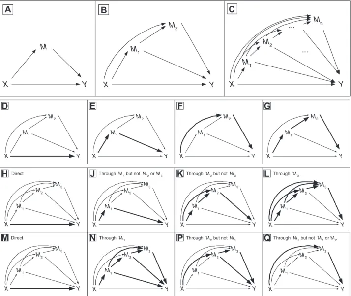
Robins and Greenland (1992) and Pearl (2001) used poten-tial outcomes (Neyman, 1923; Rubin, 1978) to give model-free definitions of direct and indirect effect estimands. Informally, a direct effect acts around a mediating variable of interest, whereas the indirect effect acts through this mediator; “di-rect” thus refers to all other pathways other than through the mediator being considered. The mediator could be mul-tivariate, but if so its constituent variables are considereden bloc: the direct effect acts around them all, and the indirect effect is through at least one of them without being further disentangled (Figure 1A).

In a setting with two mediators, M1 and M2 (see Fig-ure 1B), there are four possible pathways from exposFig-ure (X) to outcome (Y): throughM1alone, throughM2alone, through both and through neither. In this article, our primary aim is to express the total causal effect ofX onY as the sum of separate effects along each of the possible pathways: thefinest possible decomposition. The existing literature on multiple (>2) pathways from exposure to outcome can be character-ized as follows; either (1)M2 is the mediator of interest, and M1 is treated as a mediator–outcome confounder affected by exposure, leading to a coarser two-way decomposition into an effect (indirect) throughM2and an effect (direct) not through M2(Tchetgen Tchetgen and Shpitser, 2012; Vansteelandt and VanderWeele, 2013; VanderWeele and Chiba, 2014; Vander-Weele, Vansteelandt, and Robins, 2014), (2) path-specific effects are estimated, but not in such a way that their sum equals the total causal effect (Avin, Shpitser, and Pearl, 2005; Albert and Nelson, 2011), and (3) the multiple mediators do not causally affect one another (MacKinnon, 2000; Preacher and Hayes, 2008), that is, the arrow fromM1toM2in Figure 1B is assumed absent, reducing the number of path-specific effects to three. Imai and Yamamoto (2013) fall into all three categories in different sections of their article, but at no point discuss the finest possible decomposition of the total causal effect in the presence of the arrow fromM1 toM2.

The outline for the remainder of the article is as follows. In Section 2 we briefly review mediation estimands in the single mediator setting. In Section 3 we give our proposed ©2014 The Authors Biometrics published by Wiley Periodicals, Inc. on behalf of International Biometric Society

This is an open access article under the terms of the Creative Commons Attribution License, which permits use, distribution and reproduction in any medium, provided the original work is properly cited.

X

Y

M

M

X

Y

M

X

Y

M

M

M

...

...

Direct Through M₁ Through M₂ but not M₁ Through M₃ but not M₁ or M₂

X Y M₁ M₃ M₂ X Y M₁ M₃ M₂ X Y M₁ M₃ M₂ X Y M₁ M₃ M₂

Direct Through M1 but not M2 or M3 Through M2 but not M3 Through M3

X Y M₁ M2 X Y M₁ M2 X Y M₁ M2 X Y M₁ M2

A

B

C

D

H

M

N

P

Q

J

K

L

E

F

G

Figure 1. Top line: representations of mediation with (A) one, (B) two, and (C)nmediators, causally ordered. Second line: a depiction of mediation through two causally ordered mediators, with each of the four paths from XtoY highlighted; (D) shows the direct path (through neitherM1norM2), (E) the indirect path throughM1alone, (F) the indirect path throughM2 alone, and (G) the indirect path through bothM1 andM2. Lines 3 and 4: an illustration of the two possible ways of defining mediator-specific natural effects through three mediators. (H)–(L) show the first way and (M)–(Q) the second.

classification of estimands when there are two causally or-dered mediators, showing how decomposition can be achieved, and suggesting strategies for reducing complexity. Section 4 gives sufficient assumptions under which the estimands in-troduced in Section 3 can be identified, including details of a sensitivity analysis, and estimation methods are discussed briefly in Section 5. The approach is illustrated in Section 6 using data from the Izhevsk Family Study, and we conclude with some discursive remarks in Section 7. Extensions to n causally ordered mediators (Figure 1C) are given in the Web Appendix.

2. A Brief Review of Causal Mediation

Estimands for One Mediator

We briefly review mediation estimands for a single mediator. A more detailed account is given in Daniel et al. (2014).

Consider an exposureX, mediatorM and outcomeY (Fig-ure 1A). The total, direct and indirect effects defined by Robins, Mark, and Newey (1992) and Pearl (2001) involve the counterfactual variablesM(x),Y(x),Y(x, m), andY(x, M(x)). These are, respectively, the valueMwould take wereXset to x, the valueY would take wereXset tox, the valueY would take wereXset toxandMtom, and the valueY would take wereXset toxandM toM(x).

For simplicity, we take X to be binary. The controlled direct effect (CDE) at level m of M is E{Y(1, m)− Y(0, m)}, the pure natural direct effect (PNDE) is EY(1, M(0))−Y(0, M(0)), and the total natural direct effect (TNDE) isEY(1, M(1))−Y(0, M(1)). In each defi-nition,Mtakes the same value in both halves of the contrast, corresponding to a “direct” effect. For the CDE, this value ofM is the same for all individuals, whereas for the natural

direct effects, it differs by individual, according to the value that M would naturally take were X set to 0 (pure) or 1 (total).

The pure natural indirect effect (PNIE) is E{Y(0, M(1))−Y(0, M(0))} and the total natural indirect effect

(TNIE) isEY(1, M(1))−Y(1, M(0)). Note that these cor-respond to the idea of an indirect (mediated) effect, since they capture the effect onY of changingX, but only via its effect onM. The first argument of the counterfactual is the same in both halves of each contrast, but this fixed value can be either 0 (pure) or 1 (total).

Note that the sum of the PNDE and TNIE and the sum of the TNDE and PNIE are the same, and that this quantity is the total causal effect (TCE) of X on Y: PNDE+TNIE=TNDE+PNIE=E{Y(1, M(1))− Y(0, M(0))} =EY(1)−Y(0)=TCE. That is, there are two definitions (pure and total) of natural direct and indirect effects, and two ways of decomposing the TCE into a sum of a natural direct and indirect effect. VanderWeele (2013) shows that the difference TNDE−PNDE=TNIE−PNIE corresponds to a “mediated interaction,” non-zero if and only if there is an effect ofXonM and an interaction betweenX andMin their effect onY. Thus the choice between the defini-tions/decompositions, which (in many contexts) is somewhat arbitrary, amounts to assigning the mediated interaction ei-ther to the direct or indirect effect.

3. Causal Mediation Estimands with Two

Causally Ordered Mediators

Turning to the setting with two mediators (Figure 1B) we first note thatM1 can affectM2 but not vice versa; in some applications, there may be doubt as to the direction of the arrow between M1 and M2, which would introduce further difficulties beyond the scope of this article. We define four

path-specific effects—one not mediated by either M1 or M2 (Figure 1D), one throughM1 alone (Figure 1E), one through M2alone (Figure 1F), and one through bothM1andM2 (Fig-ure 1G)—such that these sum to the TCE.

3.1. Potential Values of Mediators and Outcome

Let M1(x), M2(x, m1), Y(x, m1, m2), M2(x, M1(x)), and Y(x, M1(x), M2(x, M1(x))) be defined according to the ob-vious extensions of the definitions given in Section 2.

3.2. Natural Direct Effects

Let the natural-000 direct effect through neither M1 nor M2be NDE-000=E{Y(1, M1(0), M2(0, M1(0)))−Y(0, M1(0), M2(0, M1(0)))}. This is the obvious extension of the PNDE to two mediators and is the direct effect defined by Avin et al. (2005) and Albert and Nelson (2011). The first argument is the only one that changes, from 1 to 0, making it a direct effect. The other three arguments are fixed at 0; this is why we label it “000.” Rather than two types of effect (pure and total), there are now 8 types of effect—000, 100, 010, 001, 110, 101, 011, and 111—corresponding to each of the ways in which the other three arguments could be set. See Table 1 for all 8 definitions.

3.3. Indirect Effects that Allow Decomposition

We now define indirect effects through M1 alone, M2 alone, and through both M1 and M2 such that their sum, together with the natural-000 direct effect, is equal to the TCE.

The natural-100 indirect effect through M1 alone is NIE1-100=E{Y(1, M1(1), M2(0, M1(0)))−Y(1, M1(0), M2(0, M1(0)))}. Intuitively, this corresponds to an indirect effect of XonY viaM1alone since it captures the effect ofXonYonly through its effect onM1, with the effect ofM1onM2removed. The argument that differs between the two potential outcomes is the second one, thexshown here:Y(·, M1(x), M2(·, M1(·))). The first argument is set to 1 in both potential outcomes, whereas the arguments that follow x are set to 0; this is why we label it “100.” Similarly, the natural-110 indirect effect through M2 alone is NIE2-110=E{Y(1, M1(1), M2(1, M1(0)))−Y(1, M1(1), M2(0, M1(0)))}, and the natural-111

indirect effect through bothM1 andM2is NIE12-111=E{Y(1, M1(1), M2(1, M1(1)))−Y(1, M1(1), M2(1, M1(0)))}, with each of the seven other types given in Table 1. Note that only the 000 effects have been defined in previous literature (Avin et al., 2005; Albert and Nelson, 2011).

For each effect type, we define its level to be the sum of the three fixedx-arguments. Thus NDE-000 is a level-0 effect, NIE1-100 is a level-1 effect, etc.

Using the effects chosen above, it is easily verified that the total causal effect decomposes:

TCE=NDE-000+NIE1-100+NIE2-110+NIE12-111. (1) Note that Albert and Nelson (2011) study NDE-000+ NIE1-000+NIE2-000+NIE12-000, and calculate each path-specific 000 effect as a proportion of this sum. Since this sum is not in general equal to the total causal effect, these pro-portions are not analogous to the “proportion mediated” typ-ically calculated in settings with one mediator (Pearl, 2001). 3.4. Alternative Decompositions

The decomposition given in (1) is not the only such decom-position. With one mediator there are two types (pure and total) of two path-specific effects (direct and indirect); with two mediators, there are eight types of four path-specific ef-fects. Forming sums by choosing one type of each effect, with one mediator, we found that two out of the four possible sums equate to the TCE (PNDE+TNIE=TNDE+PNIE=TCE, but PNDE+PNIE=TCE and TNDE+TNIE=TCE). With two mediators, there are 84_{=4096 possible sums, and 24 of them} equate to the TCE. That is, there are exactly 24 ways of decomposing the TCE into a sum of its path-specific compo-nents through and around two mediators: the decomposition shown in (1) and 23 others (see Table 2). That these 24 are unique and represent all possible decompositions follows from the more general argument (for n mediators) given in Web Appendix A, where we show that there are (2n_{)! ways of} de-composing a TCE into a sum of path-specific effects through nmediators.

With n=2, each decomposition includes one level-0, one level-1, one level-2, and one level-3 effect. In short, there are 4!=24 ways of allocating these four levels to the four paths, and this gives rise to the 24 possible decompositions.

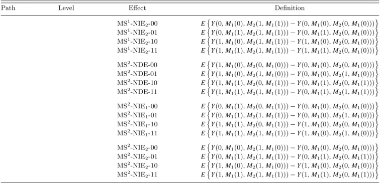
Table 1

The top half of this table gives the definitions of all natural path-specific effects when there are two causally ordered mediators. There are eight versions (one level-0, three level-1, three level-2, and one level-3) of each of the four effects (direct, indirect through M1 alone, indirect throughM2 alone, and indirect through both M1 andM2). The ones shown in bold are the

ones defined in Sections3.2and3.3. Note that the level-0effects are those studied by Avin et al. (2005) and Albert and Nelson (2011). The bottom half of the table gives the definitions of the mediator-specific effects introduced in Section3.6.3.

Path Level Effect Definition

0 NDE-000 EY(1, M1(0), M2(0, M1(0)))−Y(0, M1(0), M2(0, M1(0))) 1 NDE-100 EY(1, M1(1), M2(0, M1(0)))−Y(0, M1(1), M2(0, M1(0))) 1 NDE-010 EY(1, M1(0), M2(1, M1(0)))−Y(0, M1(0), M2(1, M1(0))) Direct 1 NDE-001 EY(1, M1(0), M2(0, M1(1)))−Y(0, M1(0), M2(0, M1(1))) (through∅) 2 NDE-110 EY(1, M1(1), M2(1, M1(0)))−Y(0, M1(1), M2(1, M1(0))) 2 NDE-101 EY(1, M1(1), M2(0, M1(1)))−Y(0, M1(1), M2(0, M1(1))) 2 NDE-011 EY(1, M1(0), M2(1, M1(1)))−Y(0, M1(0), M2(1, M1(1))) 3 NDE-111 EY(1, M1(1), M2(1, M1(1)))−Y(0, M1(1), M2(1, M1(1))) 0 NIE1-000 EY(0, M1(1), M2(0, M1(0)))−Y(0, M1(0), M2(0, M1(0))) 1 NIE1-100 EY(1, M1(1), M2(0, M1(0)))−Y(1, M1(0), M2(0, M1(0))) Indirect 1 NIE1-010 EY(0, M1(1), M2(1, M1(0)))−Y(0, M1(0), M2(1, M1(0))) through 1 NIE1-001 EY(0, M1(1), M2(0, M1(1)))−Y(0, M1(0), M2(0, M1(1))) M1 2 NIE1-110 E Y(1, M1(1), M2(1, M1(0)))−Y(1, M1(0), M2(1, M1(0))) only 2 NIE1-101 EY(1, M1(1), M2(0, M1(1)))−Y(1, M1(0), M2(0, M1(1))) 2 NIE1-011 EY(0, M1(1), M2(1, M1(1)))−Y(0, M1(0), M2(1, M1(1))) 3 NIE1-111 EY(1, M1(1), M2(1, M1(1)))−Y(1, M1(0), M2(1, M1(1))) 0 NIE2-000 EY(0, M1(0), M2(1, M1(0)))−Y(0, M1(0), M2(0, M1(0))) 1 NIE2-100 EY(1, M1(0), M2(1, M1(0)))−Y(1, M1(0), M2(0, M1(0))) Indirect 1 NIE2-010 EY(0, M1(1), M2(1, M1(0)))−Y(0, M1(1), M2(0, M1(0))) through 1 NIE2-001 EY(0, M1(0), M2(1, M1(1)))−Y(0, M1(0), M2(0, M1(1))) M2 2 NIE2-110 E Y(1, M1(1), M2(1, M1(0)))−Y(1, M1(1), M2(0, M1(0))) only 2 NIE2-101 EY(1, M1(0), M2(1, M1(1)))−Y(1, M1(0), M2(0, M1(1))) 2 NIE2-011 EY(0, M1(1), M2(1, M1(1)))−Y(0, M1(1), M2(0, M1(1))) 3 NIE2-111 EY(1, M1(1), M2(1, M1(1)))−Y(1, M1(1), M2(0, M1(1))) 0 NIE12-000 EY(0, M1(0), M2(0, M1(1)))−Y(0, M1(0), M2(0, M1(0))) 1 NIE12-100 EY(1, M1(0), M2(0, M1(1)))−Y(1, M1(0), M2(0, M1(0))) Indirect 1 NIE12-010 EY(0, M1(1), M2(0, M1(1)))−Y(0, M1(1), M2(0, M1(0))) through 1 NIE12-001 EY(0, M1(0), M2(1, M1(1)))−Y(0, M1(0), M2(1, M1(0))) bothM1 2 NIE12-110 E Y(1, M1(1), M2(0, M1(1)))−Y(1, M1(1), M2(0, M1(0))) andM2 2 NIE12-101 E Y(1, M1(0), M2(1, M1(1)))−Y(1, M1(0), M2(1, M1(0))) 2 NIE12-011 EY(0, M1(1), M2(1, M1(1)))−Y(0, M1(1), M2(1, M1(0))) 3 NIE12-111 EY(1, M1(1), M2(1, M1(1)))−Y(1, M1(1), M2(1, M1(0))) MS1-NDE-00 EY(1, M1(0), M2(0, M1(0)))−Y(0, M1(0), M2(0, M1(0))) MS1-NDE-01 EY(1, M1(0), M2(1, M1(1)))−Y(0, M1(0), M2(1, M1(1))) MS1_-NDE-10 EY(1, M1(1), M2(0, M1(0)))−Y(0, M1(1), M2(0, M1(0))) MS1_-NDE-11 EY(1, M1(1), M2(1, M1(1)))−Y(0, M1(1), M2(1, M1(1))) MS1_{-NIE1-00 EY(0, M1(1), M2(0, M1(0)))−Y(0, M1(0), M2(0, M1(0)))} MS1-NIE1-01 EY(0, M1(1), M2(1, M1(1)))−Y(0, M1(0), M2(1, M1(1))) MS1-NIE1-10 EY(1, M1(1), M2(0, M1(0)))−Y(1, M1(0), M2(0, M1(0))) MS1-NIE1-11 EY(1, M1(1), M2(1, M1(1)))−Y(1, M1(0), M2(1, M1(1))) (Continued)

Table 1

Continued

Path Level Effect Definition

MS1_-NIE 2-00 E Y(0, M1(0), M2(1, M1(1)))−Y(0, M1(0), M2(0, M1(0))) MS1_-NIE2-01 EY(0, M1(1), M2(1, M1(1)))−Y(0, M1(1), M2(0, M1(0))) MS1_{-NIE2-10 EY(1, M1(0), M2(1, M1(1)))−Y(1, M} 1(0), M2(0, M1(0))) MS1_{-NIE2-11 EY(1, M1(1), M2(1, M1(1)))−Y(1, M} 1(1), M2(0, M1(0))) MS2-NDE-00 EY(1, M1(0), M2(0, M1(0)))−Y(0, M1(0), M2(0, M1(0))) MS2-NDE-01 EY(1, M1(0), M2(1, M1(0)))−Y(0, M1(0), M2(1, M1(0))) MS2-NDE-10 EY(1, M1(1), M2(0, M1(1)))−Y(0, M1(1), M2(0, M1(1))) MS2-NDE-11 EY(1, M1(1), M2(1, M1(1)))−Y(0, M1(1), M2(1, M1(1))) MS2-NIE1-00 EY(0, M1(1), M2(0, M1(1)))−Y(0, M1(0), M2(0, M1(0))) MS2-NIE1-01 EY(0, M1(1), M2(1, M1(1)))−Y(0, M1(0), M2(1, M1(0))) MS2_-NIE 1-10 E Y(1, M1(1), M2(0, M1(1)))−Y(1, M1(0), M2(0, M1(0))) MS2_-NIE1-11 EY(1, M1(1), M2(1, M1(1)))−Y(1, M1(0), M2(1, M1(0))) MS2_{-NIE2-00 EY(0, M1(0), M2(1, M1(0)))−Y(0, M} 1(0), M2(0, M1(0))) MS2-NIE2-01 EY(0, M1(1), M2(1, M1(1)))−Y(0, M1(1), M2(0, M1(1))) MS2-NIE2-10 EY(1, M1(0), M2(1, M1(0)))−Y(1, M1(0), M2(0, M1(0))) MS2-NIE2-11 EY(1, M1(1), M2(1, M1(1)))−Y(1, M1(1), M2(0, M1(1))) Table 2

All24possible decompositions of the total causal effect (TCE) into a direct effect (NDE), an indirect effect via M1 alone

(NIE1), an indirect effect viaM2 alone (NIE2), and an indirect effect via bothM1 andM2 (NIE12). In each decomposition,

there is one level-0effect, one level-1effect, one level-2effect, and one level-3effect. The definitions of each of these effects is given in Table1. In columns2–5, the effect types are labeled:1=000,2=100,3=010,4=001,5=110,6=101,7=011, and

8=111.

Effect and type

Decomposition NDE NIE1 NIE2 NIE12 TCE=

1 1 2 5 8 NDE-000+NIE1-100+NIE2-110+NIE12-111

2 1 2 8 5 NDE-000+NIE1-100+NIE2-111+NIE12-110

3 1 5 2 8 NDE-000+NIE1-110+NIE2-100+NIE12-111

4 1 6 8 2 NDE-000+NIE1-101+NIE2-111+NIE12-100

5 1 8 2 6 NDE-000+NIE1-111+NIE2-100+NIE12-101

6 1 8 6 2 NDE-000+NIE1-111+NIE2-101+NIE12-100

7 2 1 5 8 NDE-100+NIE1-000+NIE2-110+NIE12-111

8 2 1 8 5 NDE-100+NIE1-000+NIE2-111+NIE12-110

9 3 5 1 8 NDE-010+NIE1-110+NIE2-000+NIE12-111

10 3 8 1 6 NDE-010+NIE1-111+NIE2-000+NIE12-101

11 4 6 8 1 NDE-001+NIE1-101+NIE2-111+NIE12-000

12 4 8 6 1 NDE-001+NIE1-111+NIE2-101+NIE12-000

13 5 1 3 8 NDE-110+NIE1-000+NIE2-010+NIE12-111

14 5 3 1 8 NDE-110+NIE1-010+NIE2-000+NIE12-111

15 6 1 8 3 NDE-101+NIE1-000+NIE2-111+NIE12-010

16 6 4 8 1 NDE-101+NIE1-001+NIE2-111+NIE12-000

17 7 8 1 4 NDE-011+NIE1-111+NIE2-000+NIE12-001

18 7 8 4 1 NDE-011+NIE1-111+NIE2-001+NIE12-000

19 8 1 3 7 NDE-111+NIE1-000+NIE2-010+NIE12-011

20 8 1 7 3 NDE-111+NIE1-000+NIE2-011+NIE12-010

21 8 3 1 7 NDE-111+NIE1-010+NIE2-000+NIE12-011

22 8 4 7 1 NDE-111+NIE1-001+NIE2-011+NIE12-000

23 8 7 1 4 NDE-111+NIE1-011+NIE2-000+NIE12-001

3.5. Example: Linear Structural Equation Model with Interactions

For illustration, we suppose that the data were generated from a linear structural equation model with interactions (and, for simplicity, no confounders), that is, a model implying the fol-lowing conditional expectations: E(M1|X)=α0+αxX,E(M2| X, M1)=β0+βxX+βm1M1+βxm1XM1andE(Y|X, M1, M2)= γ0+γxX+γm1M1+γm2M2+γxm1XM1+γxm2XM2+γm1m2M1M2+ γxm1m2XM1M2. Note that once interaction terms (or other nonlinearities) are included in the SEM, the simple method of multiplying path coefficients to calculate path-specific effects cannot be applied (VanderWeele and Vansteelandt, 2009).

In Web Appendix B we derive each of the 32 path-specific estimands in this special case in terms of the parameters above, together with certain conditional variance/covariance terms. For example, we have that

NDE-000=γx+γxm₁α0+(γxm2+γxm1m2α0) (β0+βm1α0) +γxm₁m2βm1σ 2 m1 whereσ2 m1=Var (M1|X), and NIE2-000=γm₂βx+γm ₁m2βxα0+βxm1α0(γm2+γm1m2α0) +γm1m2βxm1σ 2 m1,

where the terms denoted by the underbraces could be set to zero by adding appropriate constants to M1 and M2 (so that α0=β0=0); although in the presence of interactions these terms differ for different effect types (see Web Ap-pendix B). Note that NIE2-000, for example, containsγm2βx,

the term that would result from applying the “product of coefficients” methods to a linear model without interactions (Wright, 1921). It also has a further term involving σ2

m1 if

there are two interactions present. A similar expression is seen for NDE-000, where the “standard” direct effect (γx) appears along with a variance term. The formulæ for some of the other effects involves the covariance ofM1(0) andM1(1); we return to this point later. Note that the natural effects derived here would coincide with those used in the LSEM approach in the absence of all interactions.

3.6. Practical Suggestions for Reducing Complexity

With two mediators, it can be feasible to estimate all 32 path-specific effects, and hence all 24 decompositions, and compare them. However, with more mediators, the complexity grows at such a rate that this becomes impractical, even for three mediators (see Web Appendix A). In this section, we give three suggestions for reducing this complexity.

3.6.1. Focusing on effects of greatest substantive interest.

Depending on the exposure, it can often be argued that the 000 effects are substantively most interesting, and easiest to interpret. For example, if X=1 denotes a new experimental medical treatment, with X=0 for the standard treatment, then the 000 effects are most naturally interpreted, since they entail setting the free arguments in the effect to what they

would be under the standard treatment. If, in addition, one particular mediator is of greater interest than the others, then the number of decompositions one needs to consider could be partially reduced by focusing only on decompositions that include level 000 of the indirect effect through the mediator of interest (e.g., forM2, decompositions 9, 10, 14, 17, 21, and 23 in Table 2). With two mediators, therefore, this strategy reduces the number of decompositions from 24 to 6.

3.6.2. Summary natural path-specific effects. We define the summary natural path-specific effects SNDE (direct), SNIE1 (through M1 only), SNIE2 (through M2 only) and SNIE12 (through bothM1 andM2) as follows:

SNDE= 1 4(NDE-000+NDE-111)+ 1 12 0<i+j+k<3 NDE-ijk, SNIE1 = 1 4(NIE1-000+NIE1-111)+ 1 12 0<i+j+k<3 NIE1-ijk,

and similarly for SNIE2 and SNIE12. The weights (1

4 and 1

12) follow from how the path-specific types contribute to each of the 24 decompositions: in columns 2–5 of Table 2, each type-1 and type-8 (000 and 111) effect appears 6 times, and each of the other effect types appears twice. It follows therefore that

SNDE+SNIE1+SNIE2+SNIE12=TCE (2) and (2) represents a summary of the 24 decompositions, which itself is a decomposition of the TCE into four (summary) path-specific effects. Whereas with one mediator, the sum-mary direct and indirect effects can be interpreted as the di-rect and indidi-rect effects that would be seen in a particular randomized experiment (see Web Appendix C), we are not aware of a similar intuitive interpretation of the summary ef-fects for two or more mediators.

When summarizing the effects in this fashion, it would be useful also to consider the variability of the component effects, so that this information is not entirely lost. For example, for the direct effects, we define:

var-NDE= 1 4

(NDE-000−SNDE)2+(NDE-111−SNDE)2

+ 1

12

0<i+j+k<3

(NDE-ijk−SNDE)2,

weighted to reflect that the SNDE will be closer to NDE-000 and NDE-111 than to the other effects. Similar expressions for var-NIE1, var-NIE2 and var-NIE12are omitted.

3.6.3. Mediator-specific natural effects. Another option is to focus on a coarser decomposition. Indeed, as the number of mediators increases, we are unlikely to be interested in each of the 2n _{path-specific effects. For example, with two} media-tors, we could combine the effect through both M1 and M2 with either the effect through M1 alone, or with the effect throughM2 alone, leaving us with a decomposition into only

three effects: the direct effect, and two mediator-specific ef-fects. Graphically, the path shown in Figure 1G could either be combined with that of Figure 1F or with that of Figure 1E. Both lead to natural nested interpretations as follows. In the former (combining G and F, which we will denote as MS1_, mediator-specific type 1) the mediator-specific direct effect is the effect through neitherM1 nor M2, the mediator-specific effect throughM1 is the effect throughM1 but not through M2, and the mediator-specific effect throughM2 is all of the effect throughM2. Similar definitions would apply to the lat-ter (combining G and E, which we will denote as MS2_{). It} is perhaps easier to understand this “nesting” argument, by generalizing to three mediators, as shown in Figure 1H–Q.

The algebraic definitions are given in the bottom half of Table 1. Note that such a sequential treatment of multiple mediators is also discussed in VanderWeele and Vansteelandt (2014).

These summaries do not assume no exposure–mediator or no mediator–mediator interactions, as would be required in linear structural equation modeling (see Web Appendix D). Discrepancies between these and estimates obtained under a no-interactions assumption would prompt more closely study-ing the original contributstudy-ing path-specific effects.

4. Assumptions That Permit Identification

4.1. Identification Assumptions

Sufficient assumptions for the identification of the TCE are: (T.1) Consistency ofXonY:Y(x)=Y ifX=x. For those

with exposure x, outcomeY and potential outcome Y(x) coincide (Rubin, 1978; Cole and Frangakis, 2009).

(T.2) No unmeasured confounding of theX–Y relationship: Formally, Y(x)⊥⊥X|C=c for all (c, x), whereCis a set of measured background confounders, not af-fected byX.

Assumption (T.1) is required for the TCE to be inter-pretable as the effect that would be seen in a hypothetical experiment in which we intervene onXin a well-defined fash-ion. The consistency assumption then states that the results are relevant for any kind of intervention which is such that it would have produced the data we have for those for whom X=xis naturally observed.

Assumption (T.2) states that, after taking into account ob-served background confoundersC, any remaining association betweenXandY can be given a causal interpretation.

This intuition carries through to the extensions of these assumptions in the remainder of this section.

For the CDE, a sufficient set of assumptions is:

(C.1) Consistency of(X, M)onY:Y(x, m)=Y ifX=xand M=m.

(C.2) No unmeasured confounding of the (X, M)–Y rela-tionship:Y(x, m)⊥⊥X|C=c for allcandY(x, m)⊥

⊥M|C=c, X=x,L=l for all (c, x,l, m), whereL

is a set of measured intermediate confounders, where “intermediate” is used to denote that Lmay be af-fected byX(but not byM).

If we assume that the data are generated from a non-parametric structural equation model (NPSEM, see Pearl, 2009; Daniel et al., 2014) then, for the identification of the PNDE, TNDE, PNIE and TNIE, a sufficient set of assump-tions is (C.1), (C.2), and, in addition:

(N.3) Consistency of XonM:M(x)=M ifX=x. (N.4) No unmeasured confounding of the X–M

relation-ship:M(x)⊥⊥X|C=c for allc.

(N.5) No mediator–outcome confounders affected by X,

that is, no intermediate confoundersL.

Without the NPSEM assumption, (N.5) is replaced by Y(x, m)⊥⊥M(x) C=c,∀c, m, x=0,1, x=0,1, which is more difficult to interpret. Either version of assumption (N.5) can be relaxed, but only under strong parametric restrictions. For further details of all aspects of this subsection, see Daniel et al. (2014).

4.2. Assumptions for Identifying Path-Specific Effects with Two Causally Ordered Mediators

4.2.1. Non-parametric identification. For the CDE with two mediators (EY(1, m1, m2)−Y(0, m1, m2)

), (C.1) and (C.2) generalize to:

(MC.1) Consistency of(X, M1, M2)onY.

(MC.2) No unmeasured confounding of the(X, M1, M2)−Y

relationship: Y(x, m1, m2)⊥⊥X|C=c for all (c, x, m1, m2), Y(x, m1, m2)⊥⊥M1|C=c, X=x,L1=l1 for all (c, x,l1, m1, m2) andY(x, m1, m2)⊥⊥M2|C=

c, X=x,L1=l1, M1=m1,L2=l2for all (c, x,l1, m1,

l2, m2), where C are measured background con-founders (unaffected byX,M1 orM2),L1 is a set of measured intermediate confounders, which may be affected byX, but not byM1, andL2is a second set of measured intermediate confounders, which may be affected byX and/orM1, but not byM2. See Web Figure 5A.

Under (MC.1) and (MC.2), the CDE is then identified using theg-computation formula (Robins, 1986); see Web Appendix E.

The generalizations of (N.3)–(N.5) (for the natural effects) to two mediators, under the assumption that the data are generated from a NPSEM, are as follows:

(MN.3) Consistency ofXonM1 and of (X, M1)onM2. (MN.4) No unmeasured confounding of the X–M1 or

(X, M1)–M2 relationships:

M1(x)⊥⊥X|C=c for all (c, x), M2(x, m1)⊥⊥ M1|C=c, X=x,L1=l1 for all (c, x,l1, m1) and M2(x, m1)⊥⊥X|C=c for all (c, x).

(MN.5) No mediator–outcome confounder affected by X,

that is, no (L1,L2) (Web Appendix F).

Each half of each of the natural path-specific effects in Table 1 is of the form

EY(x, M1(x), M2(x, M1(x)))

and thus if we could identify (3) under assumptions (MC.1), (MC.2) and (MN.3)–(MN.5), all effects in Table 1 would be identified. To this end, we have the following result:

Theorem_{1. Under assumptions (MC.1), (MC.2) and} (MN.3)–(MN.5), we have that: EY(x, M1(x), M2(x, M1(x))) = C M1 M1 M2 E{Y|C=c, X=x, M1=m1, M2=m2} ×fM2|C,X,M1 m2 c, x, m1 fM1(x)|C,M1(x)(m1|c, m1) ×fM_1|C,X m1 c, x ×fC(c) dμM2(m2) dμM1(m1) dμM1(m1) dμC(c). (4)

For the proof, see Web Appendix H.

Note that (4) involves one density (shown in a box) not written as a function of the distribution of the observed data. A sensitivity analysis when this is unknown is discussed in the next section. There are two special cases in which the boxed quantity in (4) is not required, or is trivially known.

Special case 1:x=x

If x=x, then f_M1(x)|C,M1(x)(m1|c, m1)=I(m1=m1). Thus all path-specific estimands in which x=x in both

halves of the expression are nonparametrically identified under assumptions (MC.1), (MC.2), and (MN.3)–(MN.5). These are: NDE-000, NDE-010, NDE-101, NDE-111, NIE2-000, NIE2-100, NIE2-011, and NIE2-111. Also, note that MS1 -NDE-00 and MS1_{-NDE-11, together with all of the MS}2_-NDE, MS2_-NIE

1 and MS2-NIE2 effects, are made up of effects in whichx=x, and thus are also identified under assumptions (MC.1), (MC.2) and (MN.3)–(MN.5).

Special case 2: No effect ofM1 onM2

If there is no effect of M1 onM2, the calculation above sim-plifies as follows

Corollary_{1. Under assumptions (MC.1), (MC.2), and} (MN.3)–(MN.5), if there is no effect ofM1 onM2: EY(x, M1(x), M2(x)) = C M1 M2 E{Y|C=c, X=x, M1=m1, M2=m2} ×fM2|C,X m2 c, x fM1|C,X m1 c, x fC(c) ×dμM2(m2) dμM1(m1) dμC(c).

All effects (when M1 does not affect M2) are thus nonpara-metrically identified under assumptions (MC.1), (MC.2), and (MN.3)–(MN.5).

In the absence of an effect of M1 on M2, the defini-tions and decomposidefini-tions given in Section 3 simplify. There is no longer a path through both M1 and M2, and thus the fourth argument in each half of each effect disappears. This leaves 12 effects, and 6 decompositions; the effects are

listed in Table 3, with the decompositions given in Web Ta-ble 1. Some of these effects and decompositions correspond to those given by Imai and Yamamoto (2013); in particu-lar, Imai and Yamamoto define the 00, 01, NDE-10, NDE-11, NIE1-00, NIE1-11, NIE2-00, and NIE2-11, but not the remaining 4 effects (see Table 3) and they point out that TCE=NDE-01+NIE1-00+NIE2-11=NDE-10+ NIE1-11+NIE2-00 but do not give the other four possible decompositions (see Web Table 1). A summary of the com-parison between the estimands defined and identified in the current manuscript versus those defined and identified in the previous literature is given in Web Table 2.

Note that the decompositions given in Web Table 1 apply also to the mediator-specific natural effects defined in Sec-tion 3.6.3.

As already noted, Avin et al. (2005) define only 000 effects, but, by symmetry, their identification result applies also to the 111 effects. Insofar as they can be compared, our result agrees with that of Avin et al. since they conclude that the effect along the direct pathway (X→Y) and the effect along the indirect pathway through M2 alone (X→M2→Y) are identifiable, but that the effects along the other two path-ways (X→M1→Y andX→M1→M2→Y) are not. This corresponds to what we find, since NDE-000, NDE-111, NIE2-000, and NIE2-111 are all included in our list of effects which can be estimated without the sensitivity parameter, whereas none of the NIE1 or NIE12effects is included in this list.

4.2.2. Identification and sensitivity analysis under a par-ticular parametric model. When there is an effect ofM1 on M2, the effects not listed under “special case 1” above re-quire knowledge of the boxed quantity in (4) when x=x. Under most estimation strategies (see Section 5), we would assume a parametric model for the distribution ofM1 given X and C, for example that M1|C, X ∼N(f(C, X;β), σ2), and we would estimate the parameters β and σ2 _{from data} onC,XandM1. Under assumptions (MN.3) and (MN.4) and if our model forM1|C, X is correctly specified, this gives us M1(x)|C ∼N(f(C, x;β), σ2_{) forx=0,1. In this case, in} or-der to know the boxed quantity in (4), we would need, in addi-tion to this model, the condiaddi-tional correlaaddi-tion betweenM1(0) and M1(1) givenC. There is no information in the data on the value of this correlation; a sensible approach would thus be to vary this parameter in a sensitivity analysis.

For example, consider the following form for the SEM for M1: M1=h(C, X)+UM1,0(1−X)+UM1,1X+UM1,2, for

some function h(C, X), where UM1=(UM1,0, UM1,1, UM1,2) and ⎛ ⎝ UM₁,0 UM₁,1 UM₁,2 ⎞ ⎠∼N ⎛ ⎝ ⎛ ⎝ 0 0 0 ⎞ ⎠, σ2 ⎛ ⎝ 1−κ2 _{0 0} 0 1−κ2 ₀ 0 0 κ2 ⎞ ⎠ ⎞ ⎠. Then M1(1) M1(0),C ∼N(h(c,1)+κ2_{(M1(0)−h(c,0)),} (1−κ4_)σ2_{). Note thatσ}2_{=Var (M}

1|C, X) can be estimated from the data. However, the data contain no information on κ2_{, the proportion of residual variance shared across worlds;} this becomes the sensitivity parameter, to be varied from 0 to 1. For more details, see Web Appendix J. An example of this sort of sensitivity analysis is given in Section 6.

Table 3

The definitions of all natural path-specific effects when there are two mediators that are not causally ordered. There are four versions (one level-0, two level-1, and one level-2) of each of the three effects (direct, indirect throughM1, and indirect

throughM2; note that there is no effect through bothM1 andM2 when the mediators are not causally ordered).

Path Level Effect Definition

0 NDE-00 EY(1, M1(0), M2(0))−Y(0, M1(0), M2(0)) Direct 1 NDE-10 EY(1, M1(1), M2(0))−Y(0, M1(1), M2(0)) (through∅) 1 NDE-01 EY(1, M1(0), M2(1))−Y(0, M1(0), M2(1)) 2 NDE-11 EY(1, M1(1), M2(1))−Y(0, M1(1), M2(1)) 0 NIE1-00 EY(0, M1(1), M2(0))−Y(0, M1(0), M2(0)) Indirect 1 NIE1-10 EY(1, M1(1), M2(0))−Y(1, M1(0), M2(0)) throughM1 1 NIE1-01 E Y(0, M1(1), M2(1))−Y(0, M1(0), M2(1)) 2 NIE1-11 EY(1, M1(1), M2(1))−Y(1, M1(0), M2(1)) 0 NIE2-00 E Y(0, M1(0), M2(1))−Y(0, M1(0), M2(0)) Indirect 1 NIE2-10 E Y(1, M1(0), M2(1))−Y(1, M1(0), M2(0)) throughM2 1 NIE2-01 E Y(0, M1(1), M2(1))−Y(0, M1(1), M2(0)) 2 NIE2-11 EY(1, M1(1), M2(1))−Y(1, M1(1), M2(0))

A similar approach was taken by Daniels et al. (2012), for discrete mediators by Albert and Nelson (2011), and in the context of treatment noncompliance by Roy, Hogan, and Marcus (2008). Note that this sensitivity analysis solely as-sesses sensitivity to the arbitrary choice of conditional dis-tribution of M1(1) given M1(0) and C; it does not explore sensitivity to departures from the other assumptions, namely (MC.1), (MC.2), and (MN.3)–(MN.5). An extensive literature on sensitivity analyses with respect to the single mediator ver-sions of these assumptions exists, including in the presence of mediator–outcome confounders affected by the exposure (see, e.g., Imai, Keele, and Yamamoto, 2010; Tchetgen Tchetgen and Shpitser, 2012; VanderWeele and Chiba, 2014). In future work, we will extend these sorts of sensitivity analyses to the current setting.

An alternative route to parametric identification and sen-sitivity analysis would be to extend the “no interaction” as-sumption made by Robins and Greenland (1992) and relaxed by Imai and Yamamoto (2013). Given, however, that the 24 possible decompositions differ precisely when interactions are present, assuming them away may not be as attractive.

In Web Appendix K, we show what our identification re-sults imply for the special case of the linear model with in-teractions introduced in Section 3.5, and in Web Appendix L, we show how identification is achieved, up to a set of sen-sitivity parameters, in the presence of a restricted pattern of intermediate confounding.

5. A Note on Estimation Methods

The most obvious estimation approach is to posit parametric (regression) models for each density/expectation in the identifying equations above, to estimate their parameters from the observed data (e.g., by maximum likelihood), and then to evaluate the integrals analytically. Pearl (2009) calls this approach themediation formula. Closely related to the

g-computation formula(Robins, 1986), which can be used to

estimate controlled direct effects in the presence of intermedi-ate confounding, the mediation formula makes the additional step of integrating over the (conditional counterfactual) mediator distribution, in order to obtain natural effects (VanderWeele and Vansteelandt, 2009, 2010). When the integration is too cumbersome to be done analytically, it can instead be done by Monte Carlo simulation (Robins, 1986; Imai, Keele, and Tingley, 2010; Daniel, De Stavola, and Cousens, 2011).

The advantage of relying heavily on parametric models is that this approach is efficient when all models are correct; however, as pointed out by Robins and Wasserman (1997) and further discussed by Vansteelandt, Bekaert, and Lange (2012), the disadvantage is that it can be essentially impos-sible to specify these models such that they imply a senimpos-sible parsimonious model for the direct effect of interest. For this reason, and, more generally, to reduce reliance on paramet-ric modelling assumptions, alternative semiparametparamet-ric esti-mation approaches have been suggested (van der Laan and Petersen, 2008; VanderWeele, 2009; Tchetgen Tchetgen and Shpitser, 2012; Vansteelandt et al., 2012; Zheng and van der Laan, 2012). G-computation has nevertheless turned out to be rather successful in recent empirical applications (Young et al., 2011; Westreich et al., 2012).

We therefore adopt the fully parametric approach, imple-mented by Monte Carlo simulation, extending it to handle multiple mediators and incorporating the sensitivity analysis of Section 4.2.2. In future work, semiparametric estimation methods will be explored.

6. An Illustrative Data Example: The Izhevsk

Family Study

6.1. Data and Question of Interest

The population-based controls from a case-control study con-ducted in Izhevsk, Russia (Leon et al., 2007) are used to study

the effect of heavy drinking during the previous year (defined as the consumption of >10 L ethanol) on systolic blood pressure (SBP), measured in mmHg. We decompose this into an effects via body mass index (BMI), via gamma-glutamyl transpeptidase (GGT), via both BMI and GGT, and a direct effect, that is, via other pathways. BMI is known to affect GGT (and not vice versa), and thus the set-up is as we have discussed, withM1=BMI andM2=GGT. We estimate the path-specific effects using data on 1275 men with complete information on yearly ethanol consumption (from which “heavy drinking” is derived) and all baseline confounders: age (treated as a continuous variable), socio-economic status (SES) score (the first principal component from an asset score analysis), smoking status (current/ex/never), and cigarettes per day (≤10,10–20,>20): together we label these confounders C (Leon et al., 2007). Note that in this setting there are no (measured) intermediate confounders. Subjects with missing values of BMI, GGT and/or SBP are not excluded, since these partially observed records can be incor-porated, under the missing at random assumption (Rubin, 1976). Some descriptive statistics are shown in Web Table 3. 6.2. Estimation by ParametricG-computation via

Monte Carlo Simulation

Flexible parametric models forM1|C, X,M2|C, X, M1, and Y|C, X, M1, M2 were explored. To render the normality as-sumption for the errors more tenable, M1 andM2 (i.e., BMI and GGT) were log-transformed. All models included all pos-sible two- and three-way interactions between exposure and mediators, so that the path-specific effects of different types differ as much as the data dictate. In addition, quadratic terms for the continuous variables (age, SES, BMI, and GGT) were considered where relevant, as well as interactions be-tween exposure and confounders; these were included only if they improved the AIC (see Web Appendix M).

Write E(M1|C, X)=ν1(C, X;β1), E(M2|C, X, M1)= ν2(C, X, M1;β2), and E(Y|C, X, M1, M2)=ν3(C, X, M1, M2; β3) for the conditional expectations implied by this model, and let the error variances beσ2

1,σ22 andσ32, respectively. The estimation of path-specific effects is carried out as fol-lows.

(1) Estimate the parameters (β,σ) by OLS/ML. (2) For each subject i, draw Vi from N(0, κ2_σ2

1). κ is the sensitivity parameter (see Web Appendix J), to be var-ied between 0 (no cross-world correlation conditional on

C) and 1 (perfect cross-world correlation conditional on

C).

(3) For x=0,1, draw M1,i(x) for each i from N ν1 Ci, x;β₁ +Vi,(1−κ2_)σ2 1 .

(4) For x=0,1 and x=0,1, draw M2,i(x, M1,i(x)) from N ν2 Ci, x, M1,i(x);β2 ,σ2 2 . (5) For x=0,1, x=0,1, x=0,1 and x=0,1, draw Yi(x, M1,i(x), M2,i(x, M1,i(x))) from N ν3 Ci, x, M1,i(x), M2,i(x, M1,i(x));β3 ,σ2 3 . (6) To estimate each of the 32 effectsE{Y(x, M1(x), M2(x,

M1(x)))−Y(z, M1(z), M2(z, M1(z)))}, the empirical

average across all subjects of Yi(x, M1,i(x), M2,i(x, M1,i(x)))−Yi(z, M1,i(z), M2,i(z, M1,i(z))) is found. To decrease Monte Carlo error, the simulation is done on a dataset 1000 times the size of the original (with the values ofC copied 1000 times), although the estimation of the pa-rametersσ2

1, σ 2 2, σ

2

3 is based on the original sample. Standard errors are computed using the nonparametric bootstrap. For comparison, a LSEM (with no interactions) is also fitted.

6.3. Results

The results are shown in Tables 4 and 5 and Web Figures 1 and 2. There is evidence of a total effect of heavy drinking on SBP, but the associated confidence interval is wide (mean difference 7.63 mmHg, 95% CI 3.89–11.37). Only a small pro-portion (1.7%) of the large variation in SBP across this sample of men is explained by the dichotomous heavy drinking vari-able. It is not surprising therefore that the estimates of the various path-specific effects are also imprecise. Examination of the residual distribution for each contributing associational model shows good agreement with the assumption of normal-ity while evidence for the interaction terms was weak (see Web Table 5). There is evidence of a small indirect effect through GGT alone (mean difference ranging from 2.85 to 3.10 mmHg, lower 95% confidence limit ranging from 1.05 to 1.43, upper 95% confidence limit ranging from 4.31 to 5.06), little evi-dence of path-specific effects through either BMI alone or both BMI and GGT, with the remaining part of the total effect at-tributed to a direct effect via other pathways (mean difference ranging from 5.07 to 5.25 mmHg, lower 95% confidence limit ranging from 1.35 to 1.48, upper 95% confidence limit ranging from 8.76 to 9.03). There is little variation between the eight versions of each effect. As a consequence, when we depict the 24 possible decompositions in Figure 2, they are all similar, which suggests—in this example—that conclusions about the comparative strengths of different pathways could be drawn from just one particular decomposition.

Due to the lack of important interactions, the summary ef-fects included in Table 4 and Web Figure 1 are similar to each of the 8 effects in each instance. They are also similar to the results obtained when assuming no exposure–mediator inter-actions as implicitly done when fitting a traditional LSEM and multiplying path coefficients (note however the narrower CIs in the latter, due to the assumption of no interactions). The mediator-specific effects (Table 5 and Web Figure 2) also show a similar picture, with little difference between the two ways of defining the mediator-specific effects, due to the small magnitude of the path-specific effect through both BMI and GGT.

The results appear to be insensitive to variations inκ (Ta-bles 4 and 5), and confirm that some effects do not depend onκas theory suggests (see Web Figures 16–19).

6.4. Limitations

The exposure (heavy drinking) is likely subject to misclassi-fication. This is of particular concern in mediation analyses, if either of the mediators (in this case GGT) is a good proxy

Table 4

Estimates, SEs, and95% confidence intervals for the total causal effect (TCE), followed by each of the path-specific effects we have defined. All estimates are for mean differences in SBP measured in mmHg. The results are given for three values of

the sensitivity parameter κ: 1, 0.5and0.

κ=1 κ=0.5 κ=0

Effect Estimate 95% CI Estimate 95% CI Estimate 95% CI

TCE 7.63 (3.89,11.37) 7.62 (4.04,11.20) 7.64 (4.05,11.24) NDE-000 5.08 (1.38,8.78) 5.08 (1.35,8.81) 5.09 (1.53,8.66) NDE-100 5.07 (1.35,8.79) 4.92 (1.13,8.70) 4.88 (1.25,8.51) NDE-010 5.25 (1.47,9.03) 5.25 (1.52,8.98) 5.26 (1.62,8.90) NDE-001 5.24 (1.48,9.01) 5.17 (1.45,8.90) 5.16 (1.52,8.80) NDE-110 5.11 (1.46,8.76) 4.96 (1.28,8.65) 4.91 (1.39,8.44) NDE-101 5.10 (1.44,8.77) 5.11 (1.43,8.79) 5.11 (1.59,8.62) NDE-011 5.21 (1.45,8.97) 5.14 (1.44,8.83) 5.12 (1.50,8.73) NDE-111 5.21 (1.46,8.95) 5.21 (1.53,8.89) 5.21 (1.62,8.80) SNDE 5.15 (1.57,8.73) 5.12 (1.56,8.68) 5.11 (1.68,8.54) √ var-NDE 0.07 0.10 0.11 DEnointer _{5.24 (1.72,8.76) 5.24 (1.73,8.75) 5.24 (1.86,8.62)} NIE1-000 −0.36 (−1.01,0.29) −0.23 (−1.02,0.56) −0.18 (−1.05,0.69) NIE1-100 −0.36 (−1.01,0.28) −0.50 (−1.13,0.13) −0.54 (−1.22,0.14) NIE1-010 −0.39 (−100,0.21) −0.39 (−1.06,0.28) −0.36 (−1.09,0.37) NIE1-001 −0.39 (−100,0.21) −0.42 (−1.07,0.22) −0.41 (−1.08,0.27) NIE1-110 −0.36 (−1.01,0.29) −0.23 (−1.02,0.56) −0.18 (−1.05,0.69) NIE1-101 −0.43 (−1.09,0.24) −0.50 (−1.21,0.21) −0.51 (−1.23,0.21) NIE1-011 −0.39 (−100,0.23) −0.41 (−1.03,0.22) −0.39 (−1.03,0.25) NIE1-111 −0.42 (−1.09,0.24) −0.37 (−1.10,0.36) −0.34 (−1.12,0.45) SNIE1 −0.40 (−0.98,0.18) −0.39 (−0.99,0.20) −0.37 (−0.99,0.24) √ var-NIE1 0.02 0.07 0.09 IEnointer1 −0.39 (−0.94,0.16) −0.40 (−0.96,0.15) −0.38 (−0.94,0.18) NIE2-000 2.85 (1.39,4.32) 2.86 (1.45,4.27) 2.85 (1.41,4.30) NIE2-100 3.04 (1.09,4.98) 3.04 (1.04,5.04) 3.03 (1.04,5.03) NIE2-010 2.96 (1.05,4.87) 3.03 (1.09,4.97) 3.06 (1.10,5.01) NIE2-001 2.85 (1.39,4.32) 2.86 (1.45,4.27) 2.85 (1.41,4.30) NIE2-110 2.96 (1.05,4.87) 3.03 (1.09,4.97) 3.06 (1.10,5.01) NIE2-101 3.10 (1.14,5.06) 3.18 (1.14,5.22) 3.19 (1.13,5.25) NIE2-011 2.93 (1.43,4.44) 2.94 (1.46,4.41) 2.93 (1.46,4.40) NIE2-111 3.04 (1.09,4.98) 3.04 (1.04,5.04) 3.03 (1.04,5.03) SNIE2 2.96 (1.56,4.36) 2.97 (1.56,4.38) 2.97 (1.55,4.39) √ var-NIE2 0.08 0.10 0.10 IEnointer 2 2.34 (1.27,3.41) 2.34 (1.24,3.45) 2.34 (1.26,3.42) NIE12-000 −0.05 (−0.17,0.08) −0.04 (−0.25,0.17) −0.03 (−0.32,0.25) NIE12-100 −0.05 (−0.20,0.10) 0.01 (−0.20,0.23) 0.04 (−0.24,0.32) NIE12-010 −0.12 (−0.29,0.06) −0.14 (−0.44,0.17) −0.13 (−0.51,0.24) NIE12-001 −0.05 (−0.20,0.10) 0.01 (−0.20,0.23) 0.04 (−0.24,0.32) NIE12-110 −0.12 (−0.34,0.09) 0000 (−0.35,0.36) 0.06 (−0.36,0.48) NIE12-101 −0.05 (−0.21,0.10) −0.12 (−0.44,0.20) −0.14 (−0.53,0.26) NIE12-011 −0.05 (−0.17,0.08) −0.06 (−0.26,0.15) −0.05 (−0.32,0.21) NIE12-111 −0.05 (−0.20,0.10) 0.01 (−0.20,0.23) 0.04 (−0.24,0.32) SNIE12 −0.08 (−0.22,0.05) −0.07 (−0.22,0.07) −0.06 (−0.22,0.09) √ var-NIE12 0.04 0.08 0.10 IEnointer 12 −0.07 (−0.19,0.04) −0.08 (−0.19,0.03) −0.07 (−0.19,0.04)

Table 5

Estimates, SEs, and95% confidence intervals for the total causal effect (TCE), followed by each of the mediator-specific effects we have defined. All estimates are for mean differences in SBP measured in mmHg. The results are given for three

values of the sensitivity parameterκ:1,0.5and0.

κ=1 κ=0.5 κ=0

Effect Estimate 95% CI Estimate 95% CI Estimate 95% CI

TCE 7.63 (3.89,11.37) 7.62 (4.04,11.20) 7.64 (4.05,11.24) MS1-NDE-00 5.08 (1.38,8.78) 5.08 (1.35,8.81) 5.09 (1.53,8.66) MS1-NDE-10 5.11 (1.46,8.76) 4.96 (1.28,8.65) 4.91 (1.39,8.44) MS1-NDE-01 5.24 (1.48,9.01) 5.17 (1.45,8.90) 5.16 (1.52,8.80) MS1-NDE-11 5.21 (1.46,8.95) 5.21 (1.53,8.89) 5.21 (1.62,8.80) MS1-NIE1-00 −0.39 (−100,0.21) −0.39 (−1.06,0.28) −0.36 (−1.09,0.37) MS1-NIE1-10 −0.36 (−1.01,0.28) −0.50 (−1.13,0.13) −0.54 (−1.22,0.14) MS1-NIE1-01 −0.39 (−100,0.23) −0.41 (−1.03,0.22) −0.39 (−1.03,0.25) MS1-NIE1-11 −0.42 (−1.09,0.24) −0.37 (−1.10,0.36) −0.34 (−1.12,0.45) MS1-NIE2-00 2.81 (1.35,4.26) 2.82 (1.41,4.23) 2.82 (1.38,4.26) MS1-NIE2-10 2.97 (1.09,4.86) 2.91 (0.98,4.84) 2.89 (0.98,4.8) MS1-NIE2-01 2.82 (1.35,4.28) 2.80 (1.39,4.21) 2.80 (1.36,4.24) MS1-NIE2-11 2.91 (1.03,4.79) 3.04 (1.10,4.99) 3.09 (1.11,5.08) MS2-NDE-00 5.08 (1.38,8.78) 5.08 (1.35,8.81) 5.09 (1.53,8.66) MS2-NDE-10 5.10 (1.44,8.77) 5.11 (1.43,8.79) 5.11 (1.59,8.62) MS2-NDE-01 5.25 (1.47,9.03) 5.25 (1.52,8.98) 5.26 (1.62,8.90) MS2-NDE-11 5.21 (1.46,8.95) 5.21 (1.53,8.89) 5.21 (1.62,8.80) MS2-NIE1-00 −0.51 (−1.25,0.23) −0.53 (−1.27,0.22) −0.49 (−1.25,0.26) MS2-NIE1-10 −0.49 (−1.27,0.29) −0.50 (−1.29,0.29) −0.48 (−1.30,0.34) MS2-NIE1-01 −0.43 (−1.10,0.24) −0.45 (−1.12,0.23) −0.42 (−1.11,0.27) MS2_-NIE 1-11 −0.48 (−1.2,0.24) −0.49 (−1.23,0.25) −0.47 (−1.21,0.27) MS2_-NIE 2-00 2.85 (1.39,4.32) 2.86 (1.45,4.27) 2.85 (1.41,4.30) MS2_-NIE 2-10 3.02 (1.11,4.94) 3.03 (1.06,4.99) 3.02 (1.06,4.99) MS2_-NIE 2-01 2.93 (1.43,4.44) 2.94 (1.46,4.41) 2.93 (1.46,4.40) MS2_-NIE 2-11 3.04 (1.09,4.98) 3.04 (1.04,5.04) 3.03 (1.04,5.03)

for the true exposure, leading to an inflation of the estimated indirect effect. A feature of the Izhevsk Family Study, not ex-ploited here, is that extremely rich information was collected (from both the subjects and a proxy) on the types, quanti-ties and patterns of alcohol consumption. In these analyses we used only the information on estimated total ethanol con-sumption in one year and simplified it into a binary variable (heavy/not heavy). Concerns that the indirect effect through GGT could be inflated due to GGT’s role as a good proxy for true alcohol exposure could potentially be reduced by incor-porating more of the collected alcohol information.

In this setting, assumptions (T.2), (MC.2), and (MN.4) im-ply that age, SES and smoking are sufficient to control for con-founding of the alcohol–BMI, alcohol–GGT and alcohol–SBP relationships, and that BMI and alcohol, in addition to these baseline confounders are sufficient to control for confounding of the GGT–SBP relationship. In addition, we assume that all the specified parametric models are correctly specified, and that the assumptions made regarding the missing data mechanisms justified.

7. Concluding Remarks

Researchers are often interested in a decomposition into mul-tiple path-specific effects through many mediators, but due to the focus in the causal inference literature primarily on one mediator, multiple mediator analyses are typically performed using LSEM, ignoring interactive and nonlinear effects, and often ignoring the effect of one mediator on another. We have shown that extending the mediation framework to multiple mediators gives rise to complexities (in terms of multiplic-ity of definitions) and challenges (for identification) beyond what might have been anticipated. As well as outlining these, we have provided suggestions on how to proceed in practice, via coarser decompositions and summary effects. Important future developments include extending semiparametric esti-mation approaches to estimate the effects defined here.

8. Supplementary Materials

Web Appendices, Tables and Figures, referenced in Sections 1, 3.4–3.6, 4.2, and 6.1–6.3 are available with this paper at theBiometricswebsite on Wiley Online Library.