Pathway and Network Analysis of Transcriptomic and Genomic Data

(1)

저작자표시-비영리-변경금지 2.0 대한민국 이용자는 아래의 조건을 따르는 경우에 한하여 자유롭게 l 이 저작물을 복제, 배포, 전송, 전시, 공연 및 방송할 수 있습니다. 다음과 같은 조건을 따라야 합니다: l 귀하는, 이 저작물의 재이용이나 배포의 경우, 이 저작물에 적용된 이용허락조건 을 명확하게 나타내어야 합니다. l 저작권자로부터 별도의 허가를 받으면 이러한 조건들은 적용되지 않습니다. 저작권법에 따른 이용자의 권리는 위의 내용에 의하여 영향을 받지 않습니다. 이것은 이용허락규약(Legal Code)을 이해하기 쉽게 요약한 것입니다. Disclaimer 저작자표시. 귀하는 원저작자를 표시하여야 합니다. 비영리. 귀하는 이 저작물을 영리 목적으로 이용할 수 없습니다. 변경금지. 귀하는 이 저작물을 개작, 변형 또는 가공할 수 없습니다.

(2)

Doctoral Thesis

Pathway and Network Analysis of

Transcriptomic and Genomic Data

Sora Yoon

Department of Biological Sciences

Graduate School of UNIST

2019

(3)

Pathway and Network Analysis of

Transcriptomic and Genomic Data

Sora Yoon

Department of Biological Sciences

Graduate School of UNIST

(4)

(5)

(6)

i

Abstract

The development of high-throughput technologies has enabled to produce omics data and it has facilitated the systemic analysis of biomolecules in cells. In addition, thanks to the vast amount of knowledge in molecular biology accumulated for decades, numerous biological pathways have been categorized as gene-sets. Using these omics data and pre-defined gene-sets, the pathway analysis identifies genes that are collectively altered on a gene-set level under a phenotype. It helps the biological interpretation of the phenotype, and find phenotype-related genes that are not detected by single gene-based approach. Besides, the high-throughput technologies have contributed to construct various biological networks such as the protein-protein interactions (PPIs), metabolic/cell signaling networks, gene-regulatory networks and gene co-expression networks. Using these networks, we can visualize the relationships among gene-set members and find the hub genes, or infer new biological regulatory modules.

Overall, this thesis/dissertation describes three approaches to enhance the performance of pathway and/or network analysis of transcriptomic and genomic data. First, a simple but effective method that improves the gene-permuting gene-set enrichment analysis (GSEA) of RNA-sequencing data will be addressed, which is especially useful for small replicate data. By taking absolute statistic, it greatly reduced the false positive rate caused by inter-gene correlation within gene-sets, and improved the overall discriminatory ability in gene-permuting GSEA. Next, a powerful competitive gene-set analysis tool for GWAS summary data, named GSA-SNP2, will be introduced. The z-score method applied with adjusted gene score greatly improved sensitivity compared to existing competitive gene-set analysis methods while exhibiting decent false positive control. The performance was validated using both simulation and real data. In addition, GSA-SNP2 visualizes protein interaction networks within and across the significant pathways so that the user can prioritize the core subnetworks for further mechanistic study. Finally, a novel approach to predict condition-specific miRNA target network by biclustering a large collection of mRNA fold-change data for sequence-specific targets will be introduced. The bicluster targets exhibited on average 17.0% (median 19.4%) improved gain in certainty (sensitivity + specificity). The net gain was further increased up to 32.0% (median 33.2%) by filtering them using functional network information. The analysis of cancer-related biclusters revealed that PI3K/Akt signaling pathway is strongly enriched in targets of a few miRNAs in breast cancer and diffuse large B-cell lymphoma. Among them, five independent prognostic miRNAs were identified, and repressions of bicluster targets and pathway activity by mir-29 were experimentally validated. The BiMIR database provides a useful resource to search for miRNA regulation modules for 459 human miRNAs.

(7)

(8)

iii

List of Figures

Figure 1.1. SNP association test using Chi-squared test and effect size evaluation. ... 3

Figure 1.2. Comparison of cDNA microarray and RNA-sequencing ... 5

Figure 2.1. The relationship between the mixing coefficient (alpha) and the average inter-gene correlation... 20

Figure 2.2. Performance comparison of gene-permuting GSEA methods for simulated read counts. . 22

Figure 2.3. Average receiver operating characteristic (ROC) curves. ... 24

Figure 3.1. The monotone cubic spline trend curves. ... 36

Figure 3.2. Type 1 error rate comparison. ... 40

Figure 3.3. Statistical power comparison. ... 41

Figure 3.4. Power comparison using real data. ... 44

Figure 3.5. Comparison of gene p-value distributions in the pathways that are only significant with (a) GSA-SNP2 or (b) sARTP... 46

Figure 3.6. PPI network (HIPPIE) from DIAGRAM data. ... 47

Figure 4.1. Two approaches for miRNA regulation module discovery. ... 69

Figure 4.2. Overview of the biclustering-based miRNA target prediction. ... 71

Figure 4.3. Simulation test for biclustering algorithm. ... 73

Figure 4.4. Performance of miRNA target prediction using binding sequence, biclustering, and functional networks. ... 75

Figure 4.5. Performance comparison between biclustering and anticorrelation-based methods. ... 77

(12)

vii

Supplementary Figures

Figure S2.1. Performance comparison of gene-permuting GSEA methods for simulated read counts.29

Figure S2.2. Average receiver operating characteristic (ROC) curves for two sample cases. ... 30

Figure S2.3. The effect of absolute gene-permuting GSEA... 32

Figure S3.1. Dual cubic spline illustration. ... 54

Figure S3.2. Power comparison using real data with strict significance cutoff. ... 66

Figure S4.1. Progressive bicluster extension (PBE) algorithm. ... 86

Figure S4.2. Pseudocode of Progressive Bicluster Extension ... 87

Figure S4.3. Distribution of the number of conditions, genes and density in biclusters with three different fold-change cut-offs. ... 90

Figure S4.4. ESC/iPSC biclusters searched by multiple biclustering methods. ... 94

Figure S4.5. microRNA targets in PI3K/Akt pathway (DLBCL). ... 105

(13)

viii

List of Tables

Table 1.1. Types of genetic variation ... 2

Table 1.2. Size factor of six between-sample normalization methods. ... 6

Table 1.3. Popular pathway databases ... 8

Table 1.4. Competitive and self-contained gene-set analysis methods for gene expression data. ... 10

Table 1.5. Competitive and self-contained gene-set analysis methods for GWAS summary data... 11

Table 2.1. Significant gene-sets detected by the absolute GSEA-GP filtering (FDR<0.1) with the mod-t score (DHT-treated and control LNCaP cell line). ... 26

Table 3.1. Power comparison using canonical pathways for diabetes. ... 45

(14)

ix

Supplementary Tables

Table S3.1. Gene Ontology terms (mSigDB C5 v6.0) related to 15 height-related categories ... 58

Table S3.2. Canonical pathways (mSigDB C2 v6.0) related to 15 T2D-related pathways ... 64

Table S4.1. Existing miRNA target prediction tools ... 83

Table S4.2. Statistics of BiMIR biclusters. ... 91

Table S4.3. Real data analysis. ... 95

Table S4.4. Let-7c bicluster targets regulating pluripotency or up-regulated in ES/iPS cells. ... 98

Table S4.5. The accuracy for bicluster targets of eleven test miRNAs ... 100

Table S4.6. The accuracy of 1.3-fold bicluster targets filtered by node degree ... 101

Table S4.9. microRNA expression patterns in cancers reported from the literature ... 104

Table S4.10. Functional enrichment test for miR-29, miR-34a, miR-145 targets in DLBCL ... 106

Table S4.11. Functional enrichment test for miR-1, miR-29, miR-34a, miR-145 targets in breast cancer ... 107

Table S4.12. Multivariate Cox regression analysis of microRNAs in the DLBCL dataset ... 108

(15)

1

Chapter I: Introduction

1.1 Omics data

A suffix ‘-ome’ represents the mass of something, and it is frequently used to indicate a group of biological molecules. For example, genome, transcriptome and proteome represent the complete sets of DNA, transcripts (RNA) and proteins in a cell, respectively. With the development of high-throughput technology, it has become possible to produce such omics data within short time. It facilitates the systematic analysis of genetic and/or epigenetic features of diseases and helps to find therapeutic and diagnostic targets. Here, the concepts and characteristics of genomic (especially for GWAS data) and transcriptomic data will be explained.

1.1.1 Genomic data

In a broad sense, the genomic data refers to any data come from genome of such as nucleotide sequences, annotations or read alignments. Among them, I will focus on the genetic variation data in this thesis/dissertation. Many diseases are caused by genetic variations (Table 1.1). The variants within coding region may alter the protein structure, and those in the non-coding regulatory region can affect to the gene expression regulation. The genomic variants are classified into two groups based on the variant size. One is the simple nucleotide variation (SNV) including single nucleotide polymorphism (SNP) and short insert/deletion. Another is the structural variation (SV) including long insert/deletion, copy number variation (CNV), inversion and translocation. Table 1.1 describes the definition and example diseases of each variant type.

The genome-wide profiling of human genetic variations has been possible with the construction of

human reference genome 1_{and two great projects such as International HapMap Projects}2_{and 1000}

Genome Project 3 _{that produced reference haplotype data for human genetic variations. In the}

International HapMap Project, more than 3 million human common SNPs had been genotyped for 1,301 individuals from 11 populations (Phase III), and identified about 500,000 tag SNPs that represent the behaviors of each linkage disequilibrium (LD) block. In 1000 Genome Project, whole genome sequencing (WGS) had been done for 2,504 individuals from 26 population, and discovered an extensive number of genomic variants including 84.7 million SNPs, 3.6 million indels and 60,000

structural variants 4_{. These reference haplotype panels are great sources for genome-wide association}

study that facilitate an efficient genotyping through imputation, which will be explained in the next section in detail.

(16)

2

Table 1.1. Types of genetic variation

Variation Type Description Example disease

Simple Nucleotide Variation (SNV)

Single nucleotide polymorphism (SNP)

Single nucleotide variation found more than 1% of population. More than 84 millions of SNPs have been found in human genome.

Sickle-cell anaemia5

Wilson’s disease6

Tay-Sachs disease7

Indel Insertion and deletion of base pairs (length: 1~10,000 bp). 1.6~2.5 millions of indels are found in human genome.

Cystic fibrosis 8

Fragile X syndrome8

muscular dystrophy8

Satellite Repetition of DNA motifs, typically 5-50 times.

• microsatellites (< 10 bp per repeat)

• minisatellites (10–60 bp per repeat)

• satellites (~hundreds bp per repeat)

• macrosatellites (several kb per repeat)

Huntington’s disease9 Fragile X syndrome9 Myotonic dystrophy9 Structural variation (SV) Copy number variation (CNV)

Copy number change of long DNA segment (>1 kb) Huntington’s disease10

Alzheimer disease11

Autism12

Inversion Rearrangement of DNA segment to reverse orientation. Haemophilia A13

Translocation Rearrangement of DNA segment to be inserted into different chromosome

Leukaemia14

Ewing’s sarcoma15

1.1.1.1 Genome-wide association study

The genome-wide association study (GWAS) is carried out to identify the genetic variants (mainly

SNPs) that are associated with a phenotype (e.g., disease) 16_{. For example, if one type of allele of a SNP}

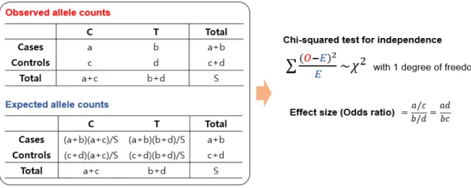
is more frequently observed in patient group compared to the control group, the SNP is regarded as a marker of the disease of interest. The higher SNP effect size (represented by odds ratio for dichotomous trait or beta value for continuous trait; figure 1.1) represents the stronger association of that SNP with the phenotype. The phenotype can be either dichotomous trait where the samples consist of case and control groups (e.g., disease vs. normal) or continuous trait such as height and BMI. For dichotomous phenotype, Chi-squared test for independence is widely performed to evaluate a SNP’s association p-value. Figure 1.1 represents the process of association test using chi-squared test for a SNP and calculating its effect size. Logistic regression is an alternative method to perform the association test. It is used to adjust various confounders such as ethnicity and batch effect. For quantitative traits, following linear regression model is used to perform association test.

Y = #$+ #&X + ( )*+* , *-$

(17)

3

where, Y is a phenotype vector, X is a (normalized) genotype vector of a SNP, +_* is confounding

factors, #_$ is intercept, #_& is regression coefficient of X and )_* is regression coefficient of

confounding factor +_*. Here, #_& represents the effect size of the SNP.

Although there are more than 84 million SNPs in human genome, we don’t need to perform association test for all of them. As mentioned in the previous section, the International HapMap Project, launched in 2003, identified ~500,000 human tag SNPs that represent each haplotype. In typical GWAS, these

tag SNPs are genotyped first using SNP array to find significantly associated tag SNPs (e.g., p <

5 × 1056_{). Next, association test is performed again for all SNPs in the haplotypes of significant tag}

SNPs. In this step, the unknown genotypes are inferred from reference panel constituted from International HapMap Project or 1000 Genome project. This step is called imputation. It enables to find more accurate SNP marker without genotyping all SNPs. SNP markers found in this discovery stage are often further validated using independent cohort.

The SNP markers identified in various phenotypes can be referred from GWAS Catalog page (https://www.ebi.ac.uk/gwas/). As of December 2018, 89,251 unique SNP-trait associations

(p-value<5 × 1056_{) are reported in GWAS Catalog.}

The result of association test for all SNPs is often provided with summarized format including columns of SNP ID, genomic position, effect allele, effect size and association p-value. This kind of data is called ‘GWAS summary data’. It is favorably used for further pathway analysis due to its relatively small data size.

Figure 1.1. SNP association test using Chi-squared test and effect size evaluation.

The tables represent the observed (denoted as O) and expected (denoted as E) SNP variant counts in

case and control samples. The association p-value of the SNP is evaluated using Chi-squared test for independence. The effect size of the SNP is calculated by odds ratio of variant counts between case and

(18)

4

1.1.2 Transcriptomic data

Various protein coding- and non-coding RNAs are transcribed from DNA in a cell. The transcriptome means the entire RNA molecules in a cell, but it usually indicates the entire set of specific RNA type of interest such as messenger RNAs (mRNAs). In this thesis/dissertation, the transcriptome represents a complete set of mRNAs. Among all RNAs, the majority is composed of ribosomal RNAs (rRNAs) and transfer RNAs (tRNAs) (95~97%), while the mRNAs that we mainly focus on occupy merely less

than 5% 17_{. Thus, the enrichment of mRNAs (or other RNA type of interest) or depletion of rRNA and}

tRNA is carried out after RNA extraction. The purified mRNA expression levels are measured by cDNA microarray or RNA-sequencing, and this transcriptomic data is used to measure (1) the expression level of transcripts in a specific condition, (2) alternative splicing to predict the isoform protein levels and (3)

the effect of genomic variants on gene expression 18-21_.

1.1.2.1 Microarray and RNA-sequencing

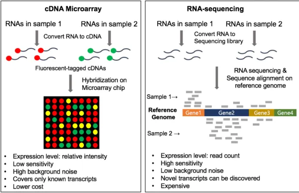
Similar to genomic data, the transcriptomic data is measured using (1) cDNA microarray or (2) RNA-sequencing (RNA-seq). The differences of two methods are represented in figure 1.2. The cDNA microarray was developed a decade earlier than RNA-seq (The first studies of cDNA microarray and

RNA-seq were published in 1995 and 2008, respectively 22-23_{). It measures all known transcripts’ levels}

at the same time based on the hybridization. Although useful, there are two limitations in this method. First, it can’t discover novel transcripts because the probes on a microarray chip are produced only for known transcripts. Second, it shows high background noises caused by nonspecific hybridization

between transcripts and probes 24_{. The RNA-seq technique was developed to solve these problems. By}

aligning the RNA fragments to the reference genome, it can discover de-novo RNA molecules 25_{. In}

addition, it shows quite low background noise and high sensitivity to detect lowly expressed RNA molecules. In spite of these advantages of RNA-seq, there are several things to be careful in analyzing RNA-seq data as described in below.

(19)

5

Figure 1.2. Comparison of cDNA microarray and RNA-sequencing 1.1.2.2 Issues in RNA-sequencing data analysis

The issues in analyzing RNA-seq data arise from its expression measuring method (counting the number of reads aligned on each gene). First issue is the normalization. It is a process to make the expression levels comparable within a sample or between samples. For example, the raw read counts of gene A and gene B within a sample cannot be directly compared because longer genes tend to be mapped with more reads. To remove this gene length bias, the raw counts of gene A and B are typically

normalized by RPKM (= 789 :;8< =>?@A×&$B

C;@; D;@CAE×D*F:8:G H*I;) or FPKM (=

J:8CK;@A =>?@A×&$B

C;@; D;@CAE×D*F:8:G H*I;). The gene length

bias is not considered when comparing the gene expression levels between samples (e.g., differential expression analysis of a gene). Instead, the ‘sequencing depth bias’ must be corrected in this case. Many

‘between-sample’ normalization methods such as DESeq26_{, TMM}27_{or UQ had been devised}

considering the library size factor. Table 1.2 represents how each method normalizes the raw read counts. Another issue is the statistical evaluation of differential expression. Because RNA-seq read counts are discrete values, Poisson distribution had been used in the early days. However, the assumption of Poisson distribution (mean and variance are same) was not fit to the real RNA-seq data where the gene count variances are often much larger than gene count means. Thus, over-dispersed Poisson distribution, a.k.a. Negative Binomial (NB) distribution, have been frequently used in modeling

RNA-seq data. In NB distribution, the variance of a i-th gene in the j-th sample (L_*MN₎_{is defined as the}

(20)

6

L*MN = P*M+ Q*P*MN

Here, Q_* is the dispersion coefficient of i-th gene. The size of dispersion coefficient depends on the

data type. For example, the dispersion coefficient of a dataset consisting of samples from unrelated individuals (e.g., cancer cohort data) will be much higher than that of those consisting of technical replicates or genetically identical samples (e.g., cell lines). Many RNA-seq DE analysis methods such

as DESeq2 28_{, edgeR}27_{, baySeq}29_{and EBSeq}30_{use the negative binomial model. Voom}31_{is another DE}

analysis method that transforms the normalized read counts to log-scale and applies the linear model which is commonly used in the microarray analysis. There are also non-parametric methods such as

NOISeq32_{or SAMseq}33_.

Table 1.2. Size factor of six between-sample normalization methods.

For each method, raw RNA-seq read count of gene g in j-th sample (R_CM) is normalized by dividing it

with size factor of j-th sample (SM). T and U represent the total number of genes and samples,

respectively. VW(x) is upper-quartile value of x, and WM is the upper-quartile count in j-th sample.

Methods Size factor of j-th sample

Total count method (TC)

SM =

∑YC-&RCM

∑YC-&∑KM-&RCM

Upper-Quartile method (UQ)

SM= VW Z

RCM

∑YC-&RCM

[ Median method (Med)

SM= U\]^_` Z RCM ∑YC-&RCM[ Quantile-normalization (Q) SM= 10D>Cabcd5( & K)∑gfhaD>Cabcf TMM logN(SM) = ∑C∈YolCMmCM ∑C∈YolCM Where mCM= logN((RCM/qM)/(RC:/q:)), lCM= ,d5rsd ,drsd + ,t5rst ,trst, qM, q: are the

total number of reads for j-th sample and reference sample r, respectively.

Tu_{is set of genes not trimmed by fold change and average expression level cutoff.}

DESeq

U\]^_` Z RCM

(∑Kv-&RCv)&/K[

1.2 Pathway analysis

One basic approach to analyze these omics data is to identify the list of genes significantly altered between case and control groups. Such analysis is called differential expression (DE) analysis for

(21)

7

transcriptomic, and GWAS for genomic data. This gene-based analysis has been widely performed to find various disease-causing genes, and extended our biological knowledges.

In addition, the pathway-based (gene-set-based) analysis provides useful information. An organism maintains its life through the complex interactions among numerous biological pathways.

Dysregulation in some metabolic pathways can lead to chronic diseases or even cancers 34_{. The pathway}

analysis is performed to find the genetic difference between case and control groups on gene-set level. There are several advantages in the pathway analysis. First, it helps easier interpretation of the common biological function of the significantly altered genes (e.g., DE genes), especially when numerous genes are significantly detected. Second, it improves the reproducibility of signature genes among

independent studies 35_{. Third, it reduces the multiple correction burden and increases the detection}

power, especially for GWAS data 36_.

1.2.1 Pathway databases

To perform pathway analysis, a list of pre-defined pathways is required. The Pathguide database (http://pathguide.org) provides links to 702 pathway databases and their information 37_{. Among them,}

251 were those of human pathway databases. Those databases are classified into 10 categories (protein-protein interactions, metabolic pathways, signaling pathways, transcription factors/ gene regulatory networks, protein-compound interactions, genetic interaction networks, protein sequence focused and others). Table 1.3 describes 13 popular pathway databases.

1.2.2 Pathway analysis methods

The pathway analysis is classified into three types based on the gene-set scoring method as follows.

1.2.2.1 Over-representation analysis

From the omics data with two sample groups, we typically identify differentially altered genes between groups using a significance cutoff (e.g., FDR<0.05). Let say such genes are signature genes. The over-representation analysis is to identify gene-sets enriched with the signature genes using hypergeometric distribution. It was popular in the early times because it was simple and useful to infer the biological theme of signature genes. DAVID is a popular web-server that performs over-representation analysis

38_{. However, the biggest problem of this approach is to set the arbitrary cutoff for signature genes.}

1.2.2.2 Functional class sorting

The cutoff-free method was devised to avoid setting such ambiguous cutoff for genes. Here, the gene-set score is directly evaluated by summarizing the gene-gene-set member’ scores obtained from omics data.

(22)

8

Besides, it is useful to detect gene-sets in which the individual genes show weak but consistent signals. Such pattern cannot be discovered using over-representation approach.

1.2.2.2.1 Gene-set enrichment analysis

One example pathway analysis method that implements the cutoff-free approach is the Gene-Set

Enrichment Analysis (GSEA)39_{. Since its paper was published in 2005, it has become the most widely}

used pathway analysis method. In GSEA, the input a priori gene-set scores (=enrichment score; ES)

are evaluated using (weighted) Kolmogorov-Smirnov (K-S) statistic, which determines score based on the relative gene score rank distribution. For example, if members of a gene-set are distributed on the top ranks, it means that gene-set is up-regulated in overall. Similarly, member gene scores are concentrated in the bottom ranks, it represents the down-regulation of that gene-set. Detailed description

for GSEA is in 2.3.1-Enrichment Score.

Table 1.3. Popular pathway databases

Database Pathway type URL Reference

Gene Ontology • Metabolic pathways

• Signalling pathways

• Protein-protein interaction

http://www.geneontology.org 40

KEGG • Metabolic pathways http://www.genome.jp/kegg/ 41

REACTOME • Metabolic pathways

• Signalling pathways

http://www.reactome.org 42

RegulonDB • Transcription Factors / Gene Regulatory Networks

http://regulondb.ccg.unam.mx/ 43

PANTHER • Signalling pathways http://www.pantherdb.org 44

Ingenuity Pathway Analysis

• Protein-Protein Interactions

• Metabolic Pathways

• Signaling Pathways

• Transcription Factors/ Gene Regulatory Networks

• Protein-Compound Interactions

https://www.qiagenbioinformatics.com/ products/ingenuity-pathway-analysis/

45

NCI PID • Signaling Pathways http://pid.nci.nih.gov/ 46

WikiPathways • Metabolic pathways

• Signalling pathways http://wikipathways.org/index.php/Wiki Pathways 47 Small Molecule Pathway DB • Metabolic pathways • Signalling pathways http://www.smpdb.ca/ 48

ConsensusPathDB • Protein-Protein Interactions

• Metabolic Pathways

• Signaling Pathways

• Transcription Factors / Gene Regulatory Networks • Protein-Compound Interactions http://cpdb.molgen.mpg.de/CPDB 49 Pathway Commons • Protein-Protein Interactions • Metabolic Pathways • Signaling Pathways • Protein-Compound Interactions http://www.pathwaycommons.org 50

(23)

9

1.2.2.3 Pathway topology-based method

In addition to over-representation analysis and functional class sorting, several methods based on pathway topology have been developed. Signaling Pathway Impact Analysis (SPIA) evaluates pathway

significance by combining two p-values obtained from over-representation test and perturbation test 51_.

CePa is a weighted gene-set analysis methods where the weights are determined by network centrality52_.

PathNet combines two types of evidences obtained from direct (p-value from DE analysis) and indirect evidence (inferred from pathway network neighborhood information) to get the signature genes. Then

pathway significance is evaluated by hypergeometric test53_{. Bayerlová et al. reported that these pathway}

topology-based methods showed better performance than classical enrichment-based methods under

simulation setting with no overlapping gene-sets, but not in other settings 54_{. It means there are rooms}

to further develop this type of pathway analysis method (although not covered in this thesis…).

1.2.3 Competitive and self-contained gene-set analysis

Before performing gene-set analysis, we have to choose proper analysis method considering the null hypothesis. There are two methods mainly concerned: the competitive and self-contained methods. The

null hypothesis (H0) of each method is as follows:

(1) H0 of competitive method: Genes in a test gene-set are not more strongly associated with phenotype

than the background genes.

(2) H0 of self-contained method: No genes in a test gene-set are associated with phenotype.

Thus, the competitive method tests the relative association of gene-sets compared to others. On the other hand, the self-contained method can significantly detect a gene-set if only few member genes are associated with the phenotype. Although it usually yields highly sensitive results, we should be careful in interpreting the result because gene-sets unrelated to phenotype can be specifically detected. Table 1.4 and 1.5 explains the gene-set analysis methods used for gene expression and GWAS data, respectively.

(24)

10

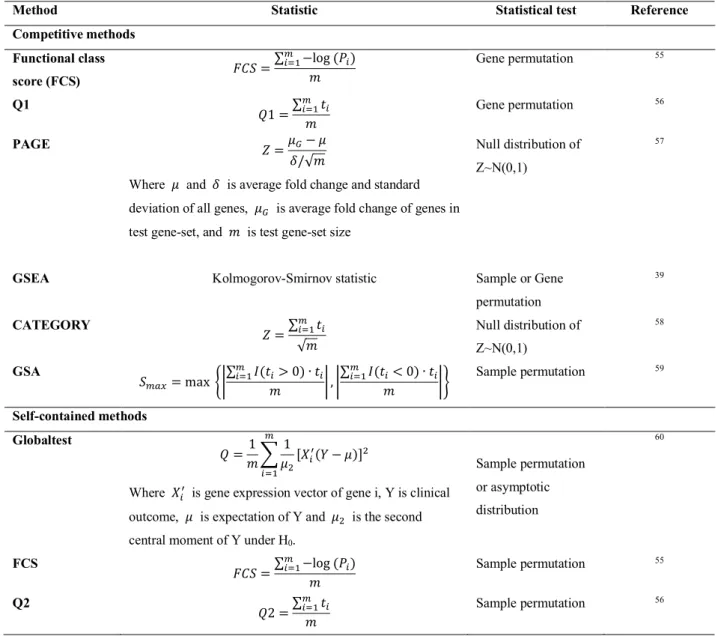
Table 1.4. Competitive and self-contained gene-set analysis methods for gene expression data.

Here, w_* and x_* are t-statistic ad p-value of gene i, respectively, and U is gene-sets size.

Method Statistic Statistical test Reference

Competitive methods Functional class score (FCS) y+z = ∑K*-&−log (x*) U Gene permutation 55 Q1 W1 =∑ w* K *-& U Gene permutation 56 PAGE _{| =}PY− P }/√U

Where P and } is average fold change and standard deviation of all genes, PY is average fold change of genes in

test gene-set, and U is test gene-set size

Null distribution of Z~N(0,1)

57

GSEA Kolmogorov-Smirnov statistic Sample or Gene

permutation 39 CATEGORY | =∑ w* K *-& √U Null distribution of Z~N(0,1) 58 GSA zK8= max ÉÑ ∑K*-&Ö(w*> 0) ∙ w* U Ñ , Ñ ∑K*-&Ö(w*< 0) ∙ w* U Ñâ Sample permutation 59 Self-contained methods Globaltest W =1 U( 1 PN[ã* u_{(å − P)]}N K *-&

Where ã*u is gene expression vector of gene i, Y is clinical

outcome, P is expectation of Y and PN is the second

central moment of Y under H0.

Sample permutation or asymptotic distribution 60 FCS y+z =∑ −log (x*) K *-& U Sample permutation 55 Q2 W2 =∑ w* K *-& U Sample permutation 56

(25)

11

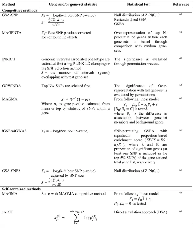
Table 1.5. Competitive and self-contained gene-set analysis methods for GWAS summary data.

Xi is the gene score of i-th gene, P and L are mean and standard deviation of all gene scores,

respectively, S is gene-set score, and m is gene-set size.

Method Gene and/or gene-set statistic Statistical test Reference

Competitive methods

GSA-SNP ã*= −log2(k-th best SNP p-value)

z = a g∑gèhaã^5ê ë/√K Null distribution of Z~N(0,1) Restandardized GSA GSEA 61

MAGENTA ã*= Best SNP p-value corrected

for confounding effects

Over-representation of top N-percentile of genes within each gene-sets is tested through comparison with random gene-sets.

62

INRICH Genomic intervals associated phenotype are estimated first using PLINK LD clumping or tag SNP selection method.

z = the number of intervals (genes) overlapping with test gene-set.

The significance is evaluated through permutation process.

63

GOWINDA Top N% SNPs are selected first The significance of

Over-representation with test gene-set is evaluated by permutations.

64

MAGMA ã*= Φ5&(1 − ì*)

Where ì* is gene p-value estimated from

mean or top îN_{-statistic of SNPs within a}

gene.

From following linear model

|H= #$H1ï⃗ + zH#H+ ó

[ò$: #H= 0] is tested.

where #H is the difference in

association between gene-set members and background genes.

65

iGSEA4GWAS ã*= −log2(best SNP p-value) SNP-permuting GSEA with

significant proportion-based enrichment score (zxöz = öz ∙ õ/R ), where k and K are proportion of significant genes (at least one SNP is included in the top 5% SNPs) of the gene-set and total gene list, respectively.

66

GSA-SNP2 ã*= −log2(k-th best SNP p-value)

adjusted by SNP size z = a g∑gèhaã^5ê ë∗_/√K Null distribution of Z~N(0,1) 67 Self-contained methods

MAGMA Same with MAGMA competitive method. From following linear model

|H= #$1ï⃗ + óH ò$: #$= 0 is tested. 65 sARTP l_Mù($)= − ( log ì_M(A)($) ûü† (°d,=¢) A-&

(26)

12

1.3 Biological network

Cells maintains life through consecutive biochemical reactions and interactions occurring among biomolecules such as metabolites, enzymes, transcription factors, signaling molecules and so on. Network is defined as a set of nodes and their relationships (edges). The interactions among biomolecules in a cell can be also represented as a complex network. There are five types of biological networks that are frequently used in bioinformatics as follows:

1) Protein-protein interaction network: The protein-protein interaction (PPI) represents the physical contact between proteins. PPIs occur in extensive cellular processes such as signal transduction, metabolism, electron transfer, transport across membranes, among others. Databases such as Database of Interacting Proteins (DIP), Biomolecular Interaction Network Database (BIND), Biological General Repository for Interaction Datasets (BioGRID), Human Protein Reference Database (HPRD), IntAct Molecular Interaction Database, Molecular Interactions Database (MINT) MIPS Protein Interaction Resource on Yeast (MIPS-MPact) and MIPS Mammalian Protein–Protein Interaction Database (MIPS-MPPI) provides validated PPI

information, 69-74_{. HIPPIE integrated these sources and provide reliable PPI information}75_.

STRING DB provides both known and predicted PPIs 76_.

2) Gene-regulatory network: This network includes regulatory relationship between regulators (e.g., transcription factor, miRNA) and their target genes. Technologies such as ChIP-chip, ChIP-seq or Clip-seq are used to identify this network. ConsensusPathDB, Ingenuity Pathway

Analysis77_{and Regulon DB provides this type of network.}

3) Gene co-expression network: It represents the co-expression modules of genes in a specific cell condition. This network is generated from microarray or RNA-seq experiments followed by gene clustering analysis.

4) Metabolic network: It is the entire set of metabolic and physiological processes (e.g., fatty acid metabolism). Thus, it comprises the network of chemical compounds and enzymes involved in

various biochemical reactions. KEGG, EcoCyc, and metaTIGER provides these networks 77-78_.

5) Signaling network: Cell signaling is a series of signal transduction that occurs within a cell or between cells to control the cellular action (e.g., PI3K/Akt signaling pathway). This process entails protein binding, phosphorylation, ubiquitination, acetylation and so on. The databases providing this network is represented in Table 1.3.

(27)

13

1.4 Research overview

Although many pathway analysis methods have been devised for gene expression or GWAS summary data, there have been still some limitations. First, most of the gene-set analysis methods for gene

expression data had been designed for microarray. For RNA-seq data, seqGSEA79_{, the use of}

log-transformed counts 31_{or pre-ranked GSEA with gene p-values from DE analysis had been suggested.}

However, there was a practical matter to apply these methods. That is, large number of RNA-seq data are composed the small number of samples due to the expensive sequencing cost. In this case, SeqGSEA, which implements sample permutation, is inappropriate to be used. Also, other two methods with gene permutation may yield many false positive results caused by inter-gene correlation among genes within same gene-set. In 2015, it was reported that the absolute statistic can effectively reduce the false positive rates in gene-permuting gene-set analysis of microarray data. In Chapter II, I tested whether GSEA with absolute gene statistic (absolute GSEA) exhibits same effect on RNA-seq data through simulation and real data analysis. For simulation test, a novel RNA-seq read count simulation method reflecting the inter-gene correlation was devised in this study. As a result, the absolute GSEA greatly improved the false positive control and overall discriminatory ability. The contents in this chapter are published in PLoS ONE in 2016 with the title ‘Improving Gene-Set Enrichment Analysis of RNA-Seq Data with

Small Replicates.’ 80

Next, I focused on the pathway analysis of GWAS summary data. Many of the competitive pathway analysis methods for GWAS summary data were too conservative to detect meaningful pathways. Some self-contained approaches were developed to increase the detection power, but there has been a concern that those methods may report gene-sets not relevant to phenotype as significant. In Chapter III, I will describe a powerful competitive gene-set analysis tools for GWAS summary data, named GSA-SNP2. By adjusting gene scores based on SNP size, it successfully increased the detection power while maintaining decent false positive control. The performance of GSA-SNP2 was validated using both simulation and real data. In addition, the GSA-SNP2 software provides gene network visualization within a gene-set or across significant gene-sets. The contents in this chapter are published in Nucleic Acids Research in 2018 with the title ‘Efficient pathway enrichment and network analysis of GWAS summary data using GSA-SNP2.’

Finally, Chapter IV describes a novel approach to infer cell condition-specific microRNA target network module by biclustering a large size of gene expression fold change profiles for a set of miRNA binding targets. The biclusters (network module) represent a set of miRNA binding motif-sharing genes commonly up-regulated (or down-regulated) under multiple cell conditions. The bicluster targets improved gain in certainty (sensitivity + specificity), and the net gain was further increased by incorporating functional network information. The analysis of cancer-related biclusters revealed that PI3K/Akt signaling pathway is strongly enriched in targets of a few miRNAs in breast cancer and

(28)

14

diffuse large B-cell lymphoma. Among them, five independent prognostic miRNAs were identified, and repressions of bicluster targets and pathway activity by mir-29 were experimentally validated. The BiMIR database provides useful search engine for biclusters of 459 human miRNAs.

(29)

15

Chapter II: Improving gene-set enrichment analysis of RNA-seq

data with small replicates

2.1 Abstract

To identify deregulated biological pathways in a disease is important to understand the pathophysiology and find therapeutic targets of the disease. The gene-set enrichment analysis (GSEA) has been widely used for biological pathway analysis of microarray data, and it is also being applied to RNA-seq data. However, due to the high-sequencing cost, most RNA-seq data contain only small number of samples so far, which leads to perform gene-permuting GSEA method (or preranked GSEA). A critical problem of this method is that it yields many false positives results originated from the inter-gene correlation within gene-sets. I demonstrate that taking the absolute gene statistic in one-tailed GSEA greatly improves the false-positive control and the overall discriminatory ability of the gene-permuting GSEA methods for RNA-seq data. A novel simulation method to generate correlated read counts within a gene-set was devised to test performance, and a dozen of currently available RNA-seq enrichment analysis methods were compared, where the proposed methods outperformed others that do not account for the inter-gene correlation. Analysis of real RNA-seq data also supported the proposed methods in terms of false positive control, ranks of true positives and biological relevance. An efficient R package (AbsFilterGSEA) coded with C++ (Rcpp) is available from CRAN.

2.2 Introduction

The RNA-sequencing (RNA-seq) technology has facilitated a systematic analysis of the transcriptome

in cells 23, 81_{. The biggest advantage of RNA-seq is much lowered background noise compared to the}

hybridization method (microarray). Thus, it has enabled more accurate quantification of gene

expression level 82_{. However, the differential expression (DE) analysis of RNA-seq data between two}

samples is not an easy task due to the different RNA composition and sequencing depth among samples as well as the discrete nature of RNA-seq data. Several between-normalization methods have been

devised to make the gene expression levels among different samples comparable 27, 83_{, and a variety of}

methods have been developed to test the DE of each gene based on discrete probability models. 28, 31, 33,

84-87_.

The gene-set analysis has been used to interpret the DE analysis result. One approach is the GO analysis that estimates the over-representation of DE genes in a pre-defined gene-sets such as Gene Ontology

(30)

16

analysis, it does not use the cutoff threshold to identify the DE genes. Instead, it utilizes the (weighted) Kolmogorov-Smirnov (K-S) statistic to test whether genes contributing to the phenotype are ‘enriched’ in each gene-set. Therefore, GSEA can detect the subtle but coordinated changes in a gene-set and has been widely used to find important pathways or functions in various diseases and cell conditions from

microarray data 61, 90-92_.

The pathway analysis methods and tools for RNA-seq have recently been devised based on methods

designed for microarray 31, 93-95_{. One of the issues in applying GSEA to RNA-seq data is the}

normalization of read count data. Voom method transforms the read counts into microarray-like data

for which most linear-model based methods developed for microarray can be applied 31_{. GSAAseqSP}

tool 94_{adopted TMM or DESeq normalization methods}27, 85_{which are able to address both the different}

depths and RNA compositions between samples. Another important thing to consider is the small sample sizes in RNA-seq data. Although the sequencing cost has been lowered so fast, it is still expensive. Thus, most laboratories have no choice but to produce only a few replicates for each

condition 96_{. The sample-permuting GSEA (GSEA-SP) is inappropriate to apply to such small replicate}

data. Instead, the gene-permuting GSEA (GSEA-GP) is used in this case. However, the GSEA-GP generates a lot of false positive gene-sets due to the inter-gene correlation in the gene expression.

In this study, it was demonstrated that the absolute gene statistic improved the false positive control

and overall discriminatory ability of GSEA-GP of RNA-seq data. Although the property was shown in

microarray data 97_{, it was not tested in RNA-seq data yet. The RNA-seq read counts were modeled and}

simulated using discrete probability (negative binomial distribution) 84, 98_{, and a simulation method to}

generate ‘correlated’ read counts within a gene-set was newly devised to compare the performance of GSEA methods for RNA-seq data. Note that the inter-gene correlation has a critical effect on the performance of gene-set level analysis, but has not been considered so far for the counting data because of the lack of such a simulation method.

Here, the one-tailed GSEA which takes the maximum positive deviation of the K-S statistic as a gene-set enrichment score was used for more precise gene-gene-set analysis. Based on this result, I also propose filtering the GSEA-GP results with those obtained from the absolute GSEA-GP to effectively reduce false positives. The performances of the absolute GSEA and its filtering method were demonstrated for simulated and real RNA-seq data.

2.3 Materials and Methods

2.3.1 Absolute gene-permuting GSEA and filtering

In many cases, the replicate size is too small in RNA-seq data to carry out GSEA-SP (e.g., n<10). In that case, the GSEA-GP is used instead. However, it produces a lot of false positive results because of

(31)

17

absolute gene statistic in GSEA-GP considerably reduces the false positive rate and improves the

overall discriminatory ability in analyzing microarray data 97_{. Therefore, it was tested whether the}

absolute statistic shows a similar effect in RNA-seq data analysis. In addition to replacing the gene

statistic with their absolute values 104_{, the absolute GSEA was modified as a one-tailed test in this study}

by considering only the ‘positive’ deviation in the K-S statistic. There are two reasons for this adjustment. First, simple substitution of gene scores by taking absolute values in GSEA can produce a small number of ‘down-regulated’ gene-sets which are meaningless in an absolute enrichment analysis. Second, it gives more precise null distribution of gene-set statistic: In the original GSEA algorithm, the maximum positive and negative deviation values are compared and only the larger absolute value between the two is selected for the gene-set score. This means the minor maximum deviation values are all excluded in constituting the gene-set null distributions. By taking only the positive deviation values, every gene-set contributes to the null distribution.

Gene scores: Four gene scores were considered for normalized read as follows: (1) Moderated t-statistic (mod-t): A modified two-sample t-statistic

w§ =_£ P*&− P*N

S§•¶£ *

where P_*@ is the mean read count of ith gene, ß_* in class `, and S§_£ is a shrinkage estimation of the

standard deviation of ß_*. This statistic is useful for small replicate data and is implemented using the

limma R package 105-106

(2) Signal-to-Noise ratio (SNR): The SNR (z_*) is calculated as

z_* = P*

&_{− P}

*N

L_*&_{+ L}

*N

where L_*@ is the standard deviation of expression values of ß* in class `.

(3) Zero-centered rank sum (Ranksum): This two-sample Wilcoxon statistic is introduced by Li and

Tibshirani33_{. For}_ß

*, the rank sum test statistic (®*) is calculated as,

®_* = ( ©_*M

M∈™a

−`&∙ (` + 1)

2

indexes in the first phenotypic class, `_& is the sample size of +_& and ` is the total sample size. Note

that E(®*) = 0.

(4) Log fold-change (logFC): Log fold-change (logy+_*) for ß_* is calculated as

logy+_* = log_NP*

&

(32)

18

Absolute GSEA: GSEA algorithm identifies functional gene-sets showing a coordinated gene expression change between case and control samples from gene expression profiles. Given gene scores, GSEA implements a (weighted) K-S statistic to calculate the enrichment score (ES) of each pre-defined gene-set.

(1) Enrichment score

Let z be a gene-set and ≠* be the gene score of ß*. Then, the enrichment score ES(z) is defined as

the maximum deviation of ì_E*A− ì_K*HH from zero, that is

öz(z) = Ømax* (ìE*A,*− ìK*HH,*) , ^∞ ±max* (ìE*A,*− ìK*HH,*)± ≥ ±min* (ìE*A,*− ìK*HH,*)± min

* (ìE*A,*− ìK*HH,*) , ^∞ ±max* (ìE*A,*− ìK*HH,*)± < ±U^`* (ìE*A,*− ìK*HH,*)±

where ìE*A,*= ( µ≠Mµ° q₇ Cd∈∂ M∑* , ìK*HH,* = ( 1 (q − q_∏) Cd∈∂π M∑* , q7= ( µ≠Mµ° Cd∈∂

q is the total number of genes in the dataset, q_∏ is the number of genes included in z and ∫ is a

weighting exponent which is set as one in this study as recommended39_{. (For the classical K-S}

statistic, ∫ = 0)

(2) ES for one-tailed absolute GSEA

The absolute GSEA is simply performed by substituting the gene scores by their absolute values, but the ranks of gene scores are quite different from the original GSEA algorithm in calculating the K-S

statistic. For the one-tailed test, only the positive deviation ES(z) = max

* ªìE*A,*− ìK*HH,*º is

considered for the gene-set score.

Then, the gene permutations are applied, and the corresponding ES’s are calculated and normalized for

evaluating the false discovery rate of each gene-set39_.

Filtering with absolute GSEA: To decrease the false positive results in the GSEA-GP, it is recommended to use the absolute GSEA-GP results for filtering false positives from the ordinary GSEA-GP results. In other words, only the gene-sets that are significant in both ordinary and the one-tailed absolute GSEA are considered significant. In this way, more reliable gene-sets with directionality can be obtained. In all the analyses presented in this paper, the same FDR cutoff is applied for both ordinary and absolute methods, but different cutoffs can also be considered for stricter or looser filtering.

2.3.2 Simulation of the read count data with the inter-gene correlation

High inter-gene correlation within sets severely increases the false positive rates in

gene-permuting gene-set analysis methods (a.k.a. competitive analysis) 99, 103_{. The inter-gene correlation of}

(33)

19

directly applied for ‘discrete’ read count data. Here, a novel simulation method for read count data with

inter-gene correlation in each gene-set is described. N=10,000 genes are considered and the replicate

sizes for the test and control groups are `_& and `_N, respectively.

Step 1. Parameter estimation and read count generation: The read count ã*M of ith gene in jth

sample has been modeled by an over-dispersed Poisson distribution, called negative binomial (NB)

distribution 84-85, 98_{denoted by}_ã

*M~qæ(P*M, L*MN) where P*M and L*MN = P*M+ Q*P*MN are the mean and

variance, respectively, and Q* ≥ 0 is the dispersion coefficient for gene ß*. Here, P*M = SMP*, where

S_M is the 'size factor' or 'scaling factor' of sample j and P_* is the expression level of ß_*. In this

simulation, all size factors S_M were set as 1 for simplicity. The mean and gene-wise dispersion

parameters of 10,000 genes (average read count>10) were estimated from TCGA kidney cancer

RNA-seq data (denoted as TCGA KIRC) 108_{. The edgeR R package was used to estimate both parameters}98_.

The read counts were generated using the R function 'rnbinom' where the inverse of the estimated

dispersion Q_* was input as the ‘size’ argument. This method generates read counts that are independent

between genes.

Step 2. Generation of read count data with the inter-gene correlation: Given a gene-set S with K

genes, the inter-gene correlation can be generated by incorporating a common variable within the

gene-set. Let P* and Q*, i=1,2,…K be the mean and tag-wise dispersion of ß* in the gene-set and +*M be

the read count generated from these parameters (Step 1). Let x∂= øì&, ìN, ⋯ , ì@a¡@¬√ be probability

values randomly sampled from the uniform distribution U(0,1). Then, for each ß_*, the probability

values in x_∂ are converted to a read count +_*M∗_,_j=1_,₂_,_…_,_`

&+`N using the inverse function of the

individual gene's distribution ã_*~NB(P_*, Q_*) such that ì_M≈ x(ã_*≤ +_*M∗_{). In short,}₊

*M∗ are generated

from the common uniform distribution via the gene-wise NB distribution. The 'correlated' read count

for ith gene in jth sample is then obtained by the weighted sum of the original count +_*M and the

‘commonly generated’ count +_*M∗_{as follows:}

M_ü…: = (1 − À) ∙ +_*M+ α ∙ +_*M∗_Õ

where α ∈ [0,1] is the mixing coefficient that determines the strength of the inter-gene correlation and

[ ] rounds the value to the nearest integer. One problem with this count is that its variance is reduced as

much as (2αN_{− 2α + 1)}_because

Var(M_ü…) ≈ (1 − À)N_{∙ Vª+}

*Mº + αN∙ Vª+*M∗º = (2αN− 2α + 1) ∙ L*MN

To remove this factor, an inflated dispersion Q_*u_{was used derived from the equation}

(2ÀN_{− 2À + 1) ∙ ªP} *+ Q*uP*Nº = P*+ Q*P*N Q*′ = 1 + Q_*P_* P_*∙ (2ÀN_{− 2À + 1)}− 1 P_*

(34)

20

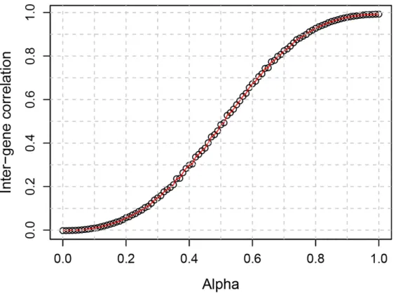
instead of Q_* in generating +_*M and +_*M∗_{. The relationship between}_À_{and inter-gene correlation is}

shown in Figure 2.1.

Figure 2.1.The relationship between the mixing coefficient (alpha) and the average inter-gene correlation.

2.3.3 Biological relevance measure of a gene-set

To measure the functional relevance of gene-sets filtered by absolute GSEA, a gene-set score based on literatures (PubMed abstract) was designed. Here, it was assumed that the significantly altered gene-sets contain genes playing important roles in the alteration of corresponding cell (tissue) condition. For

a significant gene-set z, its relevance with a specific tissue ® is scored by the log geometric average

of the abstract counts as follows:

—(z) = &

r∑ log (“”,*) r

*-& (1)

where R is the gene-set size and “”,* is the number of PubMed abstracts where both the keywords

related to the tissue ® and the name of ß_* co-occur. The literature mining was conducted using

(35)

21

2.3.4 RNA-seq data handling and gene-set condition

The RNA-seq raw read counts were normalized by the DESeq 85_{. To make the logFC stable for small}

read counts, the lower 5% of normalized counts larger than zero were added to the normalized counts. Such pseudocount does not change other types of gene scores.

2.3.5 Gene-set size

The ‘gene-set size’ represents the number of overlapping genes between the original pathway and input RNA-seq dataset. In this study, the gene-set size was constrained to 10~300.

2.3.6 AbsfilterGSEA R package

I developed a CRAN R package ‘AbsFilterGSEA’ that performs both original and absolute

gene-permuting GSEA 110_{. Here, the input raw read count matrix is normalized by DESeq method}85_{. It also}

accepts an already normalized dataset. It is quite fast because the GSEA part was implemented with

C++. The integration of C++ code to the R package was done by Rcpp package 111_.

2.4 Results

2.4.1 Comparison of gene-permuting GSEA methods for simulated read count data

The performance of twelve GSEA-GP methods for small replicate data were compared using simulation dataset reflecting the inter-gene correlation within gene-sets (See Section 2.3.2). The simulated read count data included 10,000 genes and 100 non-overlapping gene-sets each of which contained 100 genes.

First, the false positive rates (FDR < 0.1) of the GSEA-GP methods for the four gene statistics (mod-t,

SNR, Ranksum and FC) and their absolute counterparts were measured using the simulated read count datasets with four different levels of inter-gene correlation, LOW (0~0.05), 0.1, 0.3 and 0.6 within each gene-set. Two, three and five replicates in each sample group were tested and no DE genes were included. This test was repeated twenty times and their average false positive rates were depicted in Figure 2.2A and 2.2D for three and five replicates, respectively. Figure S2.1A shows the result for two-replicate case. A recently developed competitive method, Camera combined with the voom

normalization 31, 101_{, the bias-adjusted random-set method (RNA-Enrich)}95_{as well as two preranked}

GSEA methods 39_{were also compared. The preranked GSEA (unweighted) was implemented using the}

GSEA R-code 39_{where the ranks of genes were determined according to either the}_p_{-values resulted}

from the differential expression analysis using edgeR 98_{package or the simple absolute fold-changes of}

the normalized count data. Note that SeqGSEA 79_{provides only sample–permuting GSEA which is not}

(36)

22

almost same as GSEA-GP described in this paper (I checked they yielded nearly the same results for the simulated count data). Although it is described that GSAAseqSP uses the absolute gene scores, they are only used for the step-sizes in K-S statistic, and it is far from the ‘absolute’ enrichment analysis. The false positive rates of GSEA-GP for the four ordinary gene statistics and the two preranked methods showed upsurge with the increasing inter-gene correlation. However, the increase rates of false positive rates for the four absolute GSEA methods were considerably lower than those for the ordinary statistics.

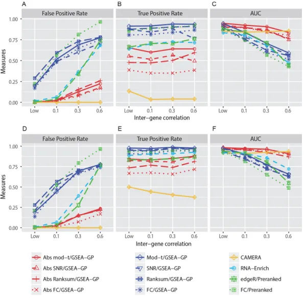
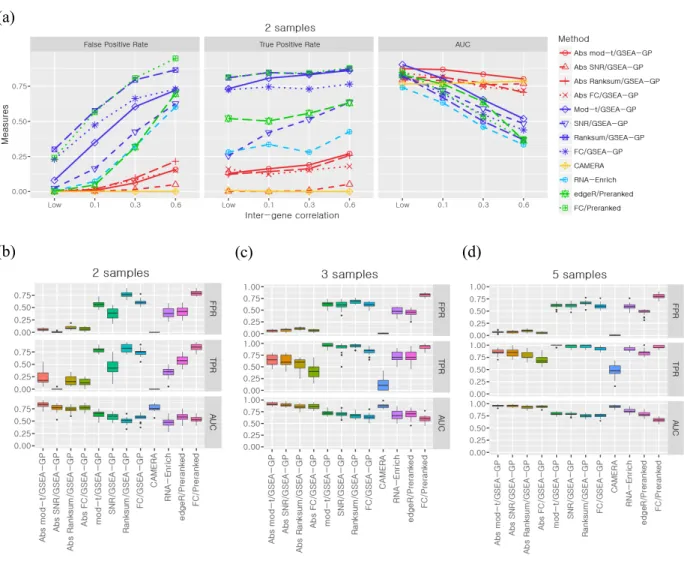
Figure 2.2. Performance comparison of gene-permuting GSEA methods for simulated read counts.

GSEA-GP methods combined with eight gene statistics, (moderated t-statistic, SNR, Ranksum, logFC and their absolute versions), Camera combined with voom normalization, RNA-Enrich and two preranked GSEA methods for edgeR p-values and FCs were compared for false positive rate, true

(37)

23

positive rate and area under the receiver operating curve using simulated read count data with three (A-C) and five replicates (D-F).

For example, when three replicates were used, even for a moderate inter-gene correlation 0.1, the false positive rates for the original statistics were approximately 50% or higher while only a few false positive sets were detected for the absolute methods (1 ~ 3%). Camera yielded no false positives for each

correlation level. Overall similar trends were observed with five replicates, but the absolute mod-t and

absolute SNR exhibited nearly the same AUCs. RNA-Enrich and the edgeR/preranked methods exhibited relatively better false positive rates compared to the GSEA-GP and FC/Preranked methods. Next, 20% of the gene-sets (20 gene-sets) in the data generated above were replaced with differentially expressed gene-sets to compare the power (true positive rate) and the overall discriminatory abilities (ROC). These gene-sets included 20~80% (uniformly at random in each gene-set) of DE genes whose mean counts in the test or control group were multiplied by 1.5~2.0 with which the read counts in the corresponding group were regenerated. In DE gene-sets, weak inter-gene correlations (0~0.05) were randomly assigned while the non-DE gene-sets were assigned with four different inter-gene correlation levels. The corresponding powers and the area under the ROC curves (AUCs) were then obtained for the twelve methods compared (Fig. 2.2B, 2.2C, 2.2E and 2.2F). The preranked GSEA with FCs and GSEA-GP methods had the highest levels of power, but their AUCs rapidly declined as the inter-gene correlation level was increased because of their poor false positive controls. With the inter-gene

correlation of 0.6, their performances were close to a random prediction (AUC≈ 0.5). On the other

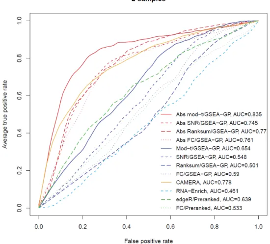
hand, the absolute GSEA-GP methods and Camera exhibited stable and good AUCs irrespective of the inter-gene correlation level. The ROC curves (average of 20 repetitions) of the twelve gene-permuting GSEA methods for the inter-gene correlation 0.3 are illustrated in Figure 2.3. For the two-replicate data, the false positive rates were similar to those of triplicate case, but the powers and AUCs were rather

lowered (Fig. S2.1a). While the mod-t still exhibited best powers and AUCs among the absolute

methods, the power of SNR was considerably lowered, which necessitates the moderated gene statistic in GSEA of small replicate data. Lastly, different inter-gene correlations were randomly assigned for gene-sets in a dataset, and two, three and five replicate cases were tested (Fig. S2.1b-d). The absolute

mod-t still exhibited best AUCs in most cases and exhibited overall similar trends as the identical correlation cases.

Overall, these results indicate that the absolute GSEA-GP provides an excellent false positive control and improves the overall discriminatory ability of GSEA-GP. Although the ordinary GSEA-GP methods exhibited best powers, they suffered from prohibitively high false positive rates resulting in very poor ranks of true positives (AUCs). Compared with Camera, the absolute methods yielded a little more false positives, but exhibited better power and overall discriminatory ability (correlation<0.6). In

(38)

24

general, for small replicate datasets, not all of the true positives may be identified perfectly by any method, but it would be important to discern some of the truly altered gene-sets reliably.

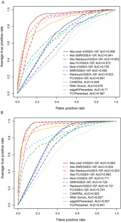
Figure 2.3. Average receiver operating characteristic (ROC) curves.

The average ROC curves (20 repetitions) of the twelve gene-permuting GSEA methods applied to simulation data with the inter-gene correlation of 0.3 for (A) three and (B) five replicate cases

(39)

25

2.4.2 Comparison of GSEA methods for RNA-seq data

The performances of GSEA methods were compared for published RNA-seq datasets in several aspects. First, two RNA-seq datasets denoted by Pickrell and Li data, respectively, were analyzed for comparing power and accuracy as follows:

The Pickrell data were generated from the lymphoblastoid cell lines of 69 unrelated Nigerian

individuals (29 male and 40 female) 112_{. To analyze the chromosomal differences in expression between}

male and female, MSigDB C1 (cytogenetic band gene-sets) 113-115_{was used for analysis. The GSEA-SP}

with SNR gene score was applied for the total dataset which resulted in two significant gene-sets ‘chryq11’ (FDR=0.00143) and ‘chrxp22’ (FDR=0.0514) both of which were sex-specific. These two gene-sets were significantly up-regulated in male and female groups, respectively. Since the GSEA-SP controls the false positives well, these two gene-sets were regarded as true positives. Then, five samples were randomly selected from each group to constitute a small replicate dataset and GSEA-GP methods with or without absolute filtering, Camera, edgeR/Preranked methods were compared for this small

replicate dataset. This process was repeated ten times. Using mod-t and logFC as the gene scores, on

average, the GSEA-GP yielded 33.9 and 19.9 significant (FDR<0.25) gene-sets including 1.5 and 1.1 true positives, respectively. On the other hand, GSEA-GP with the absolute filtering resulted in only

3.67 and 2.9 significant gene-sets which included 1.11 and 1 true positives for the mod-t and logFC

gene scores, respectively. For these five-replicate datasets, Camera did not detect any significant gene-set, and the edgeR/Preranked detected as many as 137.4 which included 1.8 true positives. This result implies that the absolute filtering method effectively reduces the false positives resulted from GSEA-GP while maintaining a good statistical power.

A similar trend was observed with the Li dataset. The Li data 116_{were generated from LNCaP cell lines}

with three samples treated with dihydrotestosterone (DHT) and four control samples. The MSigDB C2 (curated gene-set) was used for analysis and the six gene-sets containing the term ‘androgen’ were regarded as potential true positives since DHT is a kind of androgen, though there can be other truly

altered gene-sets. When the GSEA-SP with mod-t and logFC gene score was applied for this small

replicate dataset, as expected, only one and no 'androgen' gene-set was significant (FDR<0.1),

respectively. On the other hand, GSEA-GP with mod-t and logFC gene scores yielded as many as 187

and 569 significant gene-sets, respectively, which included four 'androgen' gene-sets with FDR≤0.0067.

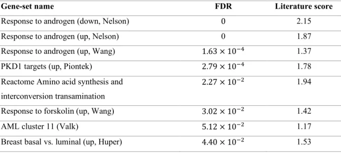
When the absolute filtering was applied, the numbers of significant gene-sets were dramatically reduced to eight (Table 2.1) and 242, which included three and four 'androgen' gene-sets, respectively. Of note,

the top three gene-sets were ‘androgen’ terms for the mod-t score. The absolute GSEA filtering with

SNR score provided a similar result. Camera detected only two 'androgen' gene-sets within 101 significant gene-sets with FDR=0.00836 and 0.0195, respectively. RNA-Enrich and edgeR/Preranked