for Bipolar Disorder Crisis Prediction
Axel Junestrand Leal
Bachelor’s Degree Final Project in Computer Science and Engineering
Trabajo de fin de grado del Grado en Ingeniería Informática
Facultad de Informática
Universidad Complutense de Madrid
Academic year 2017/2018
2
3
Index
Index ... 3 Index of figures... 6 Abstract... 10 Keywords ... 10 Resumen ... 11 Palabras clave ... 11 1. Introduction ... 12 1.1. Research context ... 12 1.2. Work plan ... 131.3. Data used for the project ... 14
1.4. Used technologies ... 14
1.4.1. Python ... 14
1.4.2. Jupyter Notebook... 14
1.5. Repository ... 15
1.6. Structure of the project ... 16
2. Introducción ... 17
2.1. Contexto de investigación ... 17
2.2. Plan de trabajo ... 18
2.3. Datos utilizados en el proyecto ... 19
2.4. Tecnologías utilizadas ... 19
2.4.1. Python ... 19
2.4.2. Jupyter Notebook... 19
2.5. Repositorio ... 19
2.6. Estructura de la memoria ... 20
3. State of the art ... 21
3.1. Similar projects and studies ... 21
3.1.1. Smartphone-based state change recognition and patient monitoring ... 21
3.1.2. Combining crisis prediction and feature importance... 21
3.1.3. Smartphone data for symptom measuring ... 21
3.1.4. Mood charting for patient monitoring ... 22
4. Data cleaning ... 23
4.1. Gathering the data ... 23
4.1.1. Episode data set ... 24
4.1.2. YMRS data set ... 24
4
4.1.4. Interview data set ... 30
4.1.5. Intervention data set ... 32
4.2. Preparing the data ... 32
4.2.1. Episode data set ... 32
4.2.2. YMRS data set ... 33
4.2.3. HDRS data set ... 33
4.2.4. Interview data set ... 34
4.2.5. Intervention data set ... 36
5. Exploratory Data Analysis ... 38
5.1. YMRS data set ... 38
5.1.1. Histograms ... 38 5.1.2. Heatmap ... 40 5.1.3. Scatterplots ... 40 5.2. HDRS data set ... 43 5.2.1. Histograms ... 43 5.2.2. Heatmap ... 44 5.2.3. Scatterplots ... 46
5.3. Interview data set ... 49
5.3.1. Histograms ... 49
5.3.2. Heatmap ... 54
5.3.3. Scatterplots ... 55
5.4. Intervention data set ... 57
5.4.1. Histograms ... 57
5.4.2. Scatterplots ... 58
6. Data combination ... 60
6.1. YMRS and Episode data sets ... 60
6.2. HDRS and Episode data sets ... 61
6.3. Interview and Episode data sets ... 62
6.4. Intervention and Episode data sets ... 64
6.5. YMRS and HDRS data sets ... 65
6.6. Interviews and Interventions ... 66
7. Application of the algorithms ... 67
7.1. Decision Tree ... 69
7.1.1. YMRS ... 70
7.1.2. HDRS ... 71
7.1.3. Interviews ... 72
5
7.1.5. YMRS-HDRS ... 74
7.1.6. Interviews-Interventions ... 75
7.1.7. Prediction accuracy comparison ... 75
7.2. Random Forest ... 76
7.2.1. Prediction accuracy comparison ... 76
7.3. SVM ... 77
7.3.1. Prediction accuracy comparison ... 78
7.4. Logistic Regression ... 79
7.4.1. Prediction accuracy comparison ... 80
7.5. Tests on randomized data ... 81
7.6. Tests on real data ... 84
8. Results ... 86
8.1. Results of the data gathering ... 86
8.2. Results of the data cleaning ... 86
8.3. Results of the Exploratory Data Analysis ... 88
8.4. Results of the data combination ... 88
8.5. Results of the algorithm implementation ... 88
9. Conclusions and future work... 90
9.1. Conclusions ... 90
9.2. Future work ... 90
10. Conclusiones y trabajo futuro ... 91
10.1. Conclusiones ... 91
10.2. Trabajo futuro... 91
6
Index of figures
Figure 1.1. Project process ... 13
Figure 1.2. Jupyter Notebook logo ... 14
Figure 1.3. Markdown and Python code in Jupyter Notebook ... 15
Figure 4.1. Sample of the original Excel file with interview data (Part1) ... 23
Figure 4.2. Sample of the original Excel file with interview data (Part 2) ... 23
Figure 4.3. Loading the data into data frames with Pandas ... 24
Figure 4.4. Mania and depression episodes in patients ... 24
Figure 4.5. Fragment of the YMRS patient data (Part 1) ... 26
Figure 4.6. Fragment of the YMRS patient data (Part 2) ... 27
Figure 4.7. Fragment of the HDRS patient data (Part 1) ... 30
Figure 4.8. Fragment of the HDRS patient data (Part 2) ... 30
Figure 4.9. Interview data (Part 1) ... 31
Figure 4.10. Interview data (Part 2) ... 31
Figure 4.11. Medical interventions ... 32
Figure 4.12. Column name translation of the Episode data set ... 32
Figure 4.13. Formatting the dates in the Episode data set ... 33
Figure 4.14. Dropping Observaciones column from the YMRS data set ... 33
Figure 4.15. Column name translation of the YMRS data set ... 33
Figure 4.16. Column name translation of the HDRS data set ... 33
Figure 4.17. Filling empty values in the HDRS data set ... 34
Figure 4.18. Column name translation of the Interview data set ... 34
Figure 4.19. Categorical value unification and mapping in the Interview data set ... 35
Figure 4.20. Calculating the amount of active time in the Interview data set ... 35
Figure 4.21. Completing missing values in the Interview data set ... 36
Figure 4.22. Column name translation of the Intervention data set ... 36
Figure 4.23. Dropping entries from interventions that patients did not attend to... 37
Figure 4.24. Taking the numerical value from the relief column ... 37
Figure 5.1. Function that returns variables in a data set that can be plotted... 38
Figure 5.2. Feature distribution in the YMRS data set ... 39
Figure 5.3. Distribution of each feature in the YMRS data set ... 39
Figure 5.4. YMRS data set correlation heatmap ... 40
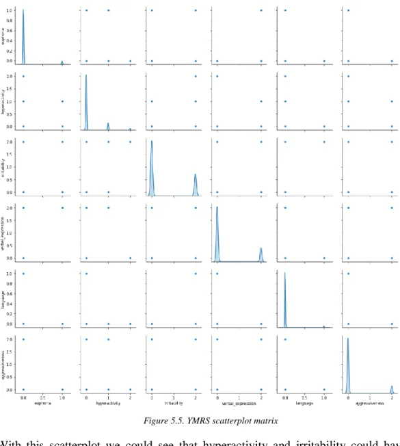
Figure 5.5. YMRS scatterplot matrix ... 41
7
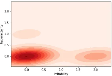
Figure 5.7. 2D kernel density plot of irritability and hyperactivity in YMRS data set .. 42
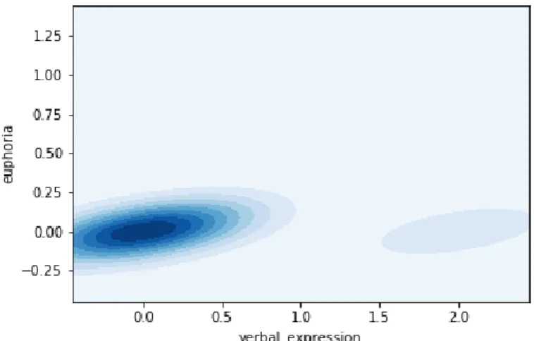
Figure 5.8. Marginal plot of verbal expression and euphoria in the YMRS data set ... 42
Figure 5.9. 2D kernel density plot of verbal expression and euphoria in the YMRS data set ... 43
Figure 5.10. Feature distribution in the HDRS data set... 43
Figure 5.11. Distribution of each feature in the HDRS data set ... 44
Figure 5.12. HDRS data set correlation heatmap ... 45
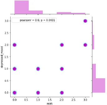
Figure 5.13. Marginal plot of depressed mood and work in the HDRS data set ... 46
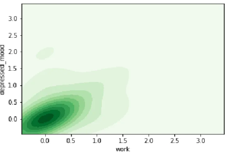
Figure 5.14. 2D kernel density plot of depressed mood and work in the HDRS data set ... 47
Figure 5.15. Marginal plot of depressed mood and psychic anxiety in the HDRS data set ... 47
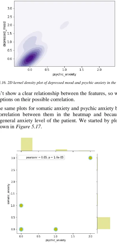
Figure 5.16. 2D kernel density plot of depressed mood and psychic anxiety in the HDRS data set ... 48
Figure 5.17. Marginal plot of somatic anxiety and psychic anxiety in the HDRS data set ... 48
Figure 5.18. 2D kernel density plot of somatic anxiety and psychic anxiety in the HDRS data set ... 49
Figure 5.19. Feature distribution in the Interview data set ... 49
Figure 5.20. Distribution of the scaled Interview data using Standard Scaler ... 50
Figure 5.21. Distribution of the scaled Interview data using Min Max Scaler... 51
Figure 5.22. Distribution of features with lowest values in the Interview data set ... 51
Figure 5.23. Distribution of the active time feature in the Interview data set ... 52
Figure 5.24. Distribution of the amount of caffeine in the Interview data set... 52
Figure 5.25. Checking if there are outliers in the Interview data set ... 53
Figure 5.26. Changing the value of the outliers in the Interview data set ... 53
Figure 5.27. Distribution of the number of cigarettes in the Interview data set ... 54
Figure 5.28. Interview data set correlation heatmap ... 54
Figure 5.29. Interviews scatterplot matrix ... 55
Figure 5.30. Marginal plot of motivation and mood in the Interview data set ... 56
Figure 5.31. 2D kernel density plot of motivation and mood in the Interview data set . 56 Figure 5.32. Feature distribution in the Intervention data set ... 57
Figure 5.33. Distribution of the scaled Intervention data using Standard Scaler ... 58
Figure 5.34. Marginal plot of relief and GAF in the Intervention data set ... 58
Figure 5.35. 2D kernel density plot of relief and GAF in the Intervention data set ... 59
Figure 6.1. Function that checks the episode a patient is in with a given date ... 60
8
Figure 6.3. Distribution of verbal expression and euphoria on different patient states in
the YMRS data set ... 61
Figure 6.4. Distribution of depressed mood and work on different patient states in the HDRS data set ... 61
Figure 6.5. Distribution of somatic and psychic anxiety on different patient states in the HDRS data set ... 62
Figure 6.6. Distribution of mood and motivation on different patient states in the Interview data set ... 62
Figure 6.7. Mood and motivation barplot with patient states in the Interview data set . 63 Figure 6.8. Anxiety and sleep quality barplot with patient states in the Interview data set ... 64
Figure 6.9. GAF and relief barplot with patient states in Intervention data set ... 64
Figure 6.10. Function that checks if there are any entries with the same date as the one passed as argument ... 65
Figure 6.11. Combination of YMRS and HDRS data sets ... 65
Figure 7.1. Diagram of the Machine Learning algorithm application process ... 68
Figure 7.2. Splitting the YMRS data set into training and testing data sets ... 68
Figure 7.3. Cross validation technique with testing set ... 69
Figure 7.4. Model training with Decision Tree classifier ... 70
Figure 7.5. Calculate model accuracy score ... 70
Figure 7.6. Decision Tree graph of YMRS data ... 71
Figure 7.7. Decision Tree graph of HDRS data ... 72
Figure 7.8. Decision Tree graph of Interview data ... 73
Figure 7.9. Decision Tree graph of Intervention data... 74
Figure 7.10. Decision Tree graph of YMRS-HDRS data ... 74
Figure 7.11. Decision Tree graph of Interviews-Interventions data ... 75
Figure 7.12. Prediction accuracies of the Decision Tree algorithm ... 76
Figure 7.13. Model training with Random Forest classifier ... 76
Figure 7.14. Prediction accuracies of the Random Forest algorithm ... 77
Figure 7.15. Finding the largest possible margin to the hyperplane... 77
Figure 7.16. Basic diagram of the SVM hyperplanes... 78
Figure 7.17. Prediction accuracies of the SVM algorithm ... 79
Figure 7.18. Basic diagram of one vs. all Multi-class Logistic Regression classification ... 80
Figure 7.19. Prediction accuracies of the Logistic Regression algorithm ... 81
Figure 7.20. Random patient interview data generation ... 81
Figure 7.21. Prediction of a Depression episode on a patient with the lowest mood value ... 82
9
Figure 7.22. Prediction of Depression episode on a patient with low mood and motivation
values ... 82
Figure 7.23. Prediction of a Mania episode on an active patient with high anxiety and irritability levels ... 83
Figure 7.24. Prediction of a Euthymic state on a patient with normal behaviour ... 83
Figure 7.25. Prediction of a Euthymic state on a patient with clear depression symptoms ... 84
Figure 7.26. Prediction of a Depression episode ... 84
Figure 7.27. Prediction of a Mania episode ... 85
Figure 7.28. Prediction of a Euthymic state ... 85
Figure 8.1. Length of the data sets after importing the data from the files ... 86
Figure 8.2. Sample of clean Episode data set ... 86
Figure 8.3. Sample of clean YMRS data set... 87
Figure 8.4. Sample of clean HDRS data set ... 87
Figure 8.5. Sample of clean Interview data set... 87
Figure 8.6. Sample of clean intervention data set... 87
Figure 8.7. Length of the combination of Interviews and Interventions ... 88
10
Abstract
Bipolar Disorder is a complex disorder that affects millions of people in the world. It is our belief that with the use of Big Data and Machine Learning we can help both patients and doctors make a better diagnosis of this illness.
The goal of this project is to apply different Machine Learning algorithms to symptom-based patient data in order to help create a prediction model. This model would make it easier for psychiatrists to decide whether their patients might be tending towards a depression or mania episode, or staying in a euthymic state.
The first part of the project consists in the process of gathering, cleaning and visualizing data from patients with Bipolar Disorder. It includes an exhaustive analysis of the data preparation which contains code snippets and plots that help understand the data better and observe the possible relationships and dependencies between them.
The second part includes the predictive analysis of the data. In this part, different Machine Learning algorithms are analysed and applied to the patient data in order to compare prediction accuracies and select the algorithms that suit the problem the most.
The main conclusion from the project is that in order to develop a predictive model with an acceptable level of confidence, it is essential to have both an understanding of the data that is being used and the theory regarding each algorithm that is applied, as well as having enough data for the algorithms to work with.
Keywords
Machine Learning, Big Data, Python, Jupyter Notebook, Bipolar Disorder, Mood disorder prediction
11
Resumen
El Trastorno Bipolar es un trastorno complejo que afecta a millones de personas en todo el mundo. Creemos que con el uso del Big Data y el Machine Learning podemos ayudar tanto a pacientes como a médicos a hacer un mejor diagnóstico de esta enfermedad.
El objetivo de este proyecto es aplicar diferentes algoritmos de Machine Learning a datos sintomáticos de pacientes para ayudar a crear un modelo de predicción. Este modelo facilitaría a los psiquiatras la posibilidad de evaluar si sus pacientes están tendiendo hacia un episodio de depresión o manía, o si se mantendrán en un estado eutímico.
La primera parte del trabajo consiste en el proceso de recolección, limpieza y visualización de datos de pacientes con Trastorno Bipolar. Contiene un análisis exhaustivo de la preparación de los datos que incluye fragmentos de código y gráficas que permiten entender mejor los datos y observar las posibles relaciones y dependencias que puede haber entre ellos.
La segunda parte incluye el análisis predictivo de los datos. En esta parte se aplican distintos algoritmos de Machine Learning para comparar su precisión y de esta manera poder elegir los algoritmos que mejor se adecúan al problema.
La principal conclusión del proyecto es que para desarrollar un modelo predictivo con un nivel de confianza aceptable, es esencial entender tanto los datos que se están usando, como la teoría relacionada con cada uno de los algoritmos que se aplica, así como tener suficientes datos para que los algoritmos funcionen correctamente.
Palabras clave
Machine Learning, Big Data, Python, Jupyter Notebook, Trastorno Bipolar, Predicción en trastornos del estado de ánimo
12
1.
Introduction
Machine Learningis becoming increasingly present in all systems that gather and process huge amounts of data, being almost an essential requirement in the development of new software applications.
One of the fields of work that could benefit from Machine Learning is, without doubt, the field of medicine. The use of Machine Learning algorithms allows the design of both classification and regression models that help with the diagnosis of different diseases, recommendation of drugs, automatic administration of drugs, etc.
On the medical branch of psychiatry, in the area of brain disorders, one of the existing disorders is Bipolar Disorder. This particular disorder is characterized by the oscillation of the patient’s mood between two states, mania and depression [1], which often come accompanied by different features, both physical and psychological.
Machine Learning is the process by which certain models are created, with the help of different algorithms, that predict values based on different features and become increasingly better in making these predictions the more data they train on.
This is why Machine Learning could be a useful tool for trying to predict the episode in which a patient might be in or tend towards with the help of different Bipolar Disorder symptoms and patient data.
1.1.
Research context
This final project springs from the Bip4cast project [2], which studies the appearance of crisis in patients with Bipolar Disorder in order to predict them. The main goal of the Bip4cast project is to be able to react in time and avoid the symptoms before the patients start to suffer from them.
There is a wide range of professionals working together on the Bip4cast project, including mathematicians, doctors and computer scientists, as well as patients with Bipolar Disorder. The project is developed by Clínica Nuestra Señora de la Paz, a non-profit center dedicated to Mental Health.
Various other research projects have been very relevant for this project, such as the design of a Bipolar Disorder Computer-Aided Diagnosis System [3], which combines different Machine Learning algorithms into a system in order to diagnose this disorder, or the Data Integration and Predictive Analysis for the Treatment of Drug Addiction [4], which includes a very thorough analysis on the preparation of data in a Machine Learning project. Other projects like the Analysis of a Predictive Model based on Google Cloud and Tensor Flow [5] present different Machine Learning techniques that have helped presenting other insights on the handling of huge amounts of data.
This project has been possible thanks to projects like the Design of a Big Data Architecture for the Prediction of Crisis in Bipolar Disorder [6] and the Introduction to Big Data and First Steps in a Big Data Project [7], which have helped facilitate the gathering of all the patient data.
The goal of the specific project described herein has been to try to predict the state a patient is in with the help of Machine Learning algorithms. The difficulty of this task is that not all patients behave equally when in a state or another, so if the prediction is not
13
completely accurate, it at least gives the psychiatrist a second opinion about the state a patient might be in or tend towards.
During the course of this project, the knowledge obtained during the Computer Science and Engineering degree has been very present, especially the one obtained with subjects like “Data Mining and the Big Data Paradigm” and “Probability and Statistics”, as well as “Data Structures and Algorithms”, because of the help it has brought in the understanding of algorithm structures and Machine Learning techniques.
1.2.
Work plan
The procedure that has been followed in this project is: data gathering, data cleaning, Exploratory Data Analysis, algorithm comparison, algorithm selection and predictions with randomized feature values (see Figure 1.1).
Figure 1.1. Project process
The first part of the project was to gather all the data needed for the process of Machine Learning, in order to later be able to clean and visualize it. After having gathered all the data required for the project, the next step was to clean it. This part is considered essential, as the data in this kind of projects almost always lacks entries or has empty values.
The next part of the project was the Exploratory Data Analysis (EDA), which helped us find the variables that were correlated and see the distribution of the data in the different data sets. This part also includes the identification of outliers, which are data points that are very distant from other points that can affect the prediction in a negative way.
Having a general understanding of how the data were represented in the data sets, the next part was to include different combinations of the data sets in order to find the features that could suit the problem the most.
The part were the algorithms were applied included the process of testing different baseline Machine Learningalgorithms on the different data set combinations. This part was crucial in order to select the algorithms that were going to be used for the predictions. The selection was based on their accuracy, which is a good way to measure their performance.
The last part of the project consisted in the model prediction. For this, we selected the algorithms that had the best testing performance and applied them on randomized patient data in order to observe how they worked. This section also included an application to test data corresponding to different states in which the patient could be in.
The quantity of data provided for the project was not enough to produce models with a high level of confidence, but the implementation has been designed as a blueprint for future projects that include larger amounts of data.
14
1.3.
Data used for the project
The data used for this project is anonymized patient data gathered by psychiatrists at Clínica Nuestra Señora de la Paz in Madrid. All the data was available in an Excel file with different sheets. The data has been gathered during medical appointments with four different patients that have Bipolar Disorder, but the goal for the future is that it is both recorded by the psychiatrists in appointments and with the help of mobile applications [7]. This way, the patients can actively participate in their own diagnosis.
1.4.
Used technologies
The programming language used in this project is Python 2.7 [8], which has a lot of libraries that make data cleaning and visualization less complicated, as well as applying Machine Learning algorithms. The environment used is Jupyter Notebook [9].
1.4.1. Python
Python [8] is a programming language that is widely used in Machine Learning. It is especially useful for data cleaning and plotting as the language is designed for legibility and ease of use.
There are quite a few libraries designed for this task, like Pandas [10], which includes a lot of methods for data frame handling, or Seaborn and Matplotlib[11], which are data plotting libraries.
Scikit-learn [12] is the Machine Learning library of choice for this project because it includes preprocessing and cross-validation tools as well as all the known baseline Machine Learningalgorithms.
1.4.2. Jupyter Notebook
Jupyter Notebook [9], the logo of which can be seen in Figure 1.2, is a web application consisting of “notebooks” that include live code. It is an interactive environment that contains both code and Markdown language to describe each code snippet.
Figure 1.2. Jupyter Notebook logo
The main reason this environment was chosen is the possibility it has for fast prototyping, because you can visualize the results very fast and in a cleaner way than with a terminal. The use of Markdown language is very useful too because it gives the option to explain each code snippet separately, as seen in Figure 1.3.
15
Figure 1.3. Markdown and Python code in Jupyter Notebook
1.5.
Repository
This project is shared in a public GitHub repository, which can be found at:
https://github.com/AxelJunes/BDCP
This repository contains:
• A detailed description of the prerequisites and installation of all the project components.
• All the anonymized data used in the project.
• The clean data generated in the data cleaning process. • The notebook used for the implementation of the project. • The Random Forest classifier exported from the notebook. • The Python script created for making predictions.
16
1.6.
Structure of the project
This work includes a detailed description of the whole process followed in this project. It has been structured in different chapters in order to make its reading easier.
Chapters 1 and 2 include an introduction, both in English and in Spanish, in which this section is included, that contains the background of the project as well as the goals and the work plan that has been followed.
Chapter 3 is the State of the Art, which mentions the latest projects and developments currently being carried out on this field. Each project is compared with this project stating the similarities and differences with it.
Chapter 4 describes the whole data cleaning process. In the first section, which corresponds to the data gathering, each data set is described thoroughly, with an exhaustive analysis of all the features. The second section represents the data preparation, in which each data set is prepared independently. This preparation includes the removal of empty columns and the process of filling empty values in the data set.
Chapter 5 includes the Exploratory Data Analysis, by which the data is visualized and analysed to get a better understanding of it. This chapter has a section for each data set obtained in chapter 4. These sections include three types of plots: histograms, heatmaps and scatterplots. Each plot includes a thorough analysis of the most interesting relationships found in it. The correlated features are plotted with marginal and kernel density plots, with their corresponding analysis.
Chapter 6 contains the combination of the different data sets and an analysis of each of these combinations explaining why they should or shouldn’t be used for the prediction. Some plots that include the distribution of the values on different patient episodes are also presented in this part, accompanied by their corresponding analysis.
Chapter 7 is the core of this project, the application of Machine Learning algorithms. This chapter contains a section for each algorithm that has been used, which includes the theory behind it as well as its application on each data set obtained in chapter 6. It also includes a section in which the algorithms are tested on randomized data. The last part of this chapter contains tests made on mocked data.
Chapter 8 presents the results obtained during this project, with a critical and reasoned discussion of each result, and their conclusions.
Chapters 9 and 10 contain a summary of the project conclusions as well as the future work that can be applied to the results obtained during this project, both in English and in Spanish.
17
2.
Introducción
El Machine Learning o Aprendizaje Automático está cada vez más presente en todos los sistemas que reúnen y procesan grandes cantidades de datos, siendo prácticamente un requisito indispensable en el desarrollo de nuevas aplicaciones software.
Uno de los ámbitos de trabajo que podría beneficiarse del uso del Machine Learning es, sin duda, la medicina. El uso de algoritmos de Machine Learning permite el diseño de modelos de clasificación y regresión que ayudan en el diagnóstico de diferentes enfermedades, la recomendación de medicamentos, la administración automática de dosis a pacientes, etc.
En la rama médica de la psiquiatría, en el área de trastornos cerebrales, uno de los trastornos existentes es el Trastorno Bipolar. Este trastorno se caracteriza por la oscilación del estado de ánimo del paciente entre dos estados, la manía y la depresión [1], los cuales a menudo vienen acompañados de diferentes características, tanto físicas como psicológicas.
El Machine Learning es el proceso mediante el cual se crean modelos, con la ayuda de diferentes algoritmos, que predicen valores basados en ciertas características y cuyas predicciones mejoran a medida que reciben más información.
Esta es la razón por la que el Machine Learning podría ser una herramienta útil para tratar de predecir el episodio en el cual se encuentra un paciente o al cual podría estar tendiendo, con la ayuda de los diferentes síntomas del Trastorno Bipolar y datos de pacientes.
2.1.
Contexto de investigación
Este trabajo surge del proyecto Bip4cast [2], el cual estudia la aparición de crisis en el Trastorno Bipolar para predecirlas. El objetivo principal del proyecto Bip4cast es poder reaccionar a tiempo y evitar los síntomas antes de que los pacientes los empiecen a sufrir. Un amplio grupo de profesionales colaboran en el proyecto Bip4cast, incluidos matemáticos, médicos e informáticos, así como pacientes con Trastorno Bipolar. El proyecto se está llevando a cabo por la Clínica Nuestra Señora de la Paz, un centro sin ánimo de lucro dedicado a la salud mental.
Numerosos proyectos de investigación han sido muy relevantes para este trabajo, como el Diseño de un Sistema de Diagnostico Asistido por Ordenador del Trastorno Bipolar [3], que combina diferentes algoritmos de Machine Learning en un sistema para diagnosticar este trastorno, o la Integración de Datos y el Análisis Predictivo para el Tratamiento de la Drogadicción [4], el cual incluye un análisis exhaustivo de la preparación de los datos en un proyecto de Machine Learning. Otros proyectos como el Análisis de un Modelo Predictivo Basado en Google Cloud y Tensor Flow [5] presentan diferentes técnicas de Machine Learning que han ayudado a dar otras visiones sobre el manejo de grandes cantidades de datos.
Este trabajo ha sido posible gracias a proyectos como el Diseño de una Arquitectura Big Data para la Predicción de Crisis en el Trastorno Bipolar [6] y la Introducción al Big Data y Primeros Pasos en un Proyecto Big Data [7], los cuales han facilitado la recogida de los datos de los pacientes.
18
El objetivo del trabajo descrito en esta memoria ha sido tratar de predecir el estado de un paciente con la ayuda de algoritmos de Machine Learning. La dificultad de esta tarea es que no todos los pacientes se comportan de la misma manera cuando se encuentran en un estado u otro, por lo que si la predicción no es correcta en su totalidad, al menos otorga al psiquiatra una segunda opinión sobre el estado en el que podría encontrarse o al que podría estar tendiendo el paciente.
Durante el transcurso de este proyecto, el conocimiento obtenido durante el Grado en Ingeniería Informática ha estado muy presente, sobre todo el obtenido en las asignaturas de “Minería de Datos y el Paradigma Big Data” y “Probabilidad y Estadística”, así como también “Estructuras de Datos y Algoritmos”, debido a la ayuda que han aportado en la comprensión de las estructuras de los algoritmos y las técnicas de Machine Learning.
2.2.
Plan de trabajo
El procedimiento seguido durante este proyecto ha sido: recopilación de los datos, limpieza de los datos, análisis exploratorio de los datos, comparación de los algoritmos, selección de los algoritmos y predicción con datos aleatorios (ver Figura 1.1).
La primera parte del proyecto consistió en recopilar todos los datos necesarios para el proceso de Machine Learning, para posteriormente poder limpiarlos y visualizarlos. Después de haber reunido todos los datos necesarios para el proyecto, el siguiente paso fue limpiarlos. Este proceso es esencial, ya que los datos recopilados para este tipo de proyecto casi siempre carecen de algunas entradas o contienen valores vacíos.
La siguiente etapa del proyecto fue el análisis exploratorio de datos, el cual nos ayudó a encontrar las variables correlacionadas y a observar la distribución de los datos en los diferentes conjuntos. Esta parte también incluye la identificación de valores atípicos, los cuales son puntos que se encuentran muy lejos del resto de datos y pueden afectar negativamente a la predicción.
Una vez comprendida la representación general de los datos de los diferentes conjuntos, el siguiente paso consistió en incluir distintas combinaciones de los conjuntos de datos para encontrar las características que más se ajustaran al problema planteado.
La parte en la que se aplicaron los algoritmos incluía el proceso mediante el cual se probaban diferentes algoritmos de Machine Learning a las combinaciones obtenidas anteriormente. Esta parte fue crucial para seleccionar los algoritmos que se iban a utilizar para las predicciones. La selección de los algoritmos se basó en la precisión de los mismos, lo cual es una buena manera de comparar su rendimiento.
La última fase del trabajo consistió en la predicción de los modelos. Para ello, seleccionamos los algoritmos que tenían mejor rendimiento con los datos de prueba y los aplicamos a datos de pacientes aleatorios para observar su funcionamiento. En esta sección también se incluyó una aplicación para probar datos correspondientes a diferentes estados reales en los que el paciente se podía encontrar.
La cantidad de datos proporcionados para el trabajo no era suficiente para producir modelos con un elevado nivel de confianza, pero la implementación se ha diseñado como una plantilla para proyectos futuros que incluyan una mayor cantidad de datos.
19
2.3.
Datos utilizados en el proyecto
Los datos utilizados en este trabajo son datos anónimos de pacientes recopilados por psiquiatras de la Clínica Nuestra Señora de la Paz, en Madrid. Todos los datos fueron proporcionados mediante un archivo Excel con diferentes hojas de cálculo. Los datos han sido recopilados durante las citas médicas de cuatro pacientes con Trastorno Bipolar, pero el objetivo para el futuro es que estos sean recogidos tanto en citas médicas como con la ayuda de aplicaciones móviles [7]. De esta forma, los pacientes pueden participar activamente en su propio diagnóstico.
2.4.
Tecnologías utilizadas
El lenguaje de programación utilizado en este proyecto es Python 2.7 [8], el cual tiene una gran cantidad de librerías que facilitan la limpieza y visualización de los datos, así como la aplicación de algoritmos de Machine Learning. El entorno utilizado ha sido Jupyter Notebook [9].
2.4.1. Python
Python [8] es un lenguaje de programación utilizado ampliamente para el Machine Learning. Es especialmente útil para la limpieza de datos y la creación de gráficas ya que está diseñado para ser legible y fácil de utilizar.
Existen bastantes librerías diseñadas para esta tarea, como Pandas [10], que incluye muchos métodos para el manejo de conjuntos de datos, o Seaborn y Matplotlib[11], que son librerías para crear gráficas.
Scikit-learn [12] es la librería de Machine Learning escogida para este proyecto ya que incluye herramientas de preprocesado y validación cruzada, así como todos los algoritmos básicos de Machine Learning conocidos.
2.4.2. Jupyter Notebook
Jupyter Notebook [9], cuyo logotipo se puede ver en la Figura 1.2, es una aplicación web que consiste en “cuadernos” que incluyen ejecución de código en vivo. Es un entorno interactivo que incluye tanto código como lenguaje de marcado para la descripción de los fragmentos de código.
La razón principal por la que se escogió este entorno es la posibilidad que ofrece para el prototipado, ya que se visualizan los resultados más rápido y de una forma más limpia que desde una consola de comandos. El uso del lenguaje de marcado también es muy útil ya que ofrece la opción de explicar cada fragmento de código por separado, como se puede ver en la Figura 1.3.
2.5.
Repositorio
Este proyecto se encuentra compartido en un repositorio público de GitHub, el cual se puede encontrar en: https://github.com/AxelJunes/BDCP
20
• Una descripción detallada de los prerrequisitos y la instalación de todos los componentes del proyecto.
• Todos los datos anonimizados que se han utilizado en el proyecto. • Los datos limpios generados durante la fase de limpieza de los datos. • El notebook utilizado para la implementación del proyecto.
• El clasificador Random Forest exportado desde el notebook. • El script de Python creado para realizer las predicciones.
2.6.
Estructura de la memoria
Esta memoria incluye una descripción detallada de todo el proceso seguido durante el proyecto. Ha sido estructurada en diferentes capítulos para facilitar su lectura.
Los capítulos 1 y 2 incluyen una introducción, en inglés y en castellano, que contiene tanto los antecedentes del proyecto, como los objetivos y el plan de trabajo seguido durante el mismo.
El capítulo 3 es el Estado del Arte, que menciona los últimos proyectos y desarrollos que se están llevando a cabo en este campo. Cada proyecto se compara con este proyecto indicando las similitudes y las diferencias con él.
El capítulo 4 describe todo el proceso de limpieza de los datos. En la primera sección, que corresponde a la recopilación de los datos, cada conjunto de datos se describe a fondo, con un análisis exhaustivo de todas las características. La segunda sección incluye la preparación de los datos, en la que cada conjunto de datos se prepara de manera independiente. Esta preparación incluye la eliminación de columnas vacías y el proceso de llenado de los valores vacíos de los conjuntos de datos.
El capítulo 5 incluye el análisis exploratorio de datos, mediante el cual se visualizan y analizan los datos para obtener una mejor comprensión de los mismos. Este capítulo tiene una subsección para cada conjunto de datos obtenido en el capítulo 4. Estas secciones presentan tres tipos de gráficas: histogramas, mapas de calor y gráficas de dispersión. Cada una de estas gráficas incluye un análisis en profundidad de las relaciones más importantes que se han encontrado entre los datos. Las variables correlacionadas se trazan también con gráficos marginales y de densidad de kernel, con su correspondiente análisis. El capítulo 6 contiene la combinación de los diferentes conjuntos de datos y un análisis de cada combinación explicando por qué se deben, o no, usar en la predicción. También se incluyen algunas gráficas con la distribución de valores durante diferentes episodios de los pacientes, acompañadas por su correspondiente análisis.
El capítulo 7 es el núcleo del proyecto, la aplicación de los algoritmos de Machine Learning. Este capítulo incluye una sección para cada algoritmo utilizado, la cual contiene la teoría correspondiente a cada uno y su aplicación sobre los conjuntos de datos obtenidos en el capítulo 6. También contiene una sección en la que se prueban los algoritmos con datos aleatorios. La última parte del proyecto presenta pruebas hechas con datos simulados.
El capítulo 8 desarrolla los resultados obtenidos durante el proyecto, con una discusión crítica y razonada de cada resultado y sus conclusiones.
Los capítulos 9 y 10 consisten en un resumen de las conclusiones del trabajo así como el trabajo futuro que se puede aplicar a los resultados obtenidos, tanto en inglés como en castellano.
21
3.
State of the art
The problem presented in this project is the prediction of a medical condition with the help of Machine Learning algorithms. This project contains the whole process of Machine Learning, ranging from data gathering to prediction, including data visualization and algorithm comparison, which can serve as a ground for other projects that are trying to predict medical conditions based on different symptoms presented by patients.
For this project to have future projection, it is important to state that the patients with Bipolar Disorder have to participate actively in gathering the data and work together with the doctors in order to get a diagnosis as accurate as possible.
3.1.
Similar projects and studies
Different projects and studies are currently being carried out within the area of mood disorder crisis prediction. It is, indeed, a very new area to which apply prediction algorithms to. There are a few studies that are related to this project as in trying to predict crisis in patients with Bipolar Disorder.
3.1.1. Smartphone-based state change recognition and patient monitoring
Some studies are trying to classify the state a patient is in and detect changes in patients with Bipolar Disorder with the help of technologies such as sensors integrated in smartphones [13]. These studies are quite similar to this one in the sense that objective data is gathered from a daily survey that the patients ought to complete [14].
If we don’t know the state in which the patients are when the data is gathered, it is very difficult to classify them in a state or another. This is why in this project we include the episodes of mania and depression of the patients according to the expertise of the psychiatrists.
3.1.2. Combining crisis prediction and feature importance
Knowing which variables are correlated and which features or parameters are important is essential when trying to build a model that will successfully predict the target of a study. The goal of these studies is to investigate which features have the highest importance in health. In order to achieve this, Machine Learning algorithms and techniques are applied for feature ranking [15].
The main difference of this project with the above-mentioned is that it not only includes a study of feature importance, but it also includes the application of different algorithms to predict the state with various combinations of these features.
3.1.3. Smartphone data for symptom measuring
These studies aim to correlate Bipolar Disorder symptoms with objective data gathered from smartphones. This includes both social and physical activities that patients have to write down every evening for a certain period of time [16].
The difference with this project is that these studies only use objective data to create a model, whereas this project only uses subjective data. It is important to include subjective
22
data in the study because every patient might not perceive the different symptoms in the same way, and the values can be contrasted with the opinion of psychiatrists.
3.1.4. Mood charting for patient monitoring
Having in mind the involvement of Bipolar Disorder patients with their own care, the objective of these studies is to give patients a better understanding of their condition with daily charts that represent their mood [17].
These projects are quite similar to this one as they try to involve the patients with their condition and make them a part of their own treatment, but they do not include the application of algorithms to check if the different mood representations are really accurate.
23
4.
Data cleaning
Data cleaning is an essential part of the Machine Learning process as it is the key to having concrete features and values for the model to work with. It is a difficult process and not as objective as other parts of the project might be. It consists mainly in giving quantitative values to qualitative features as these are the ones being passed to the model as parameters and they require a proper numerical scale. It also includes the identification of outliers and the handling of missing data. This process is divided in the gathering of the data, where each data set is explained thoroughly, and the cleaning of each data set.
4.1.
Gathering the data
The first part of the data cleaning consisted in gathering the data that we would be working with. To do so, we exported each worksheet from the Excel file that was provided by the doctor to csv format.
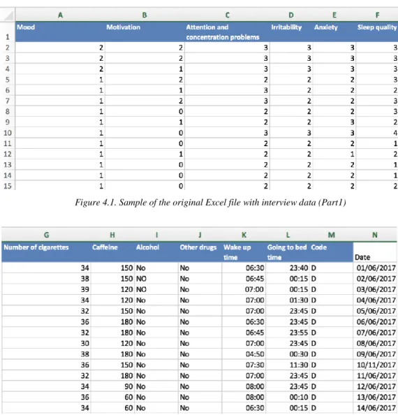
Figure 4.1. Sample of the original Excel file with interview data (Part1)
24
The initial Excel file was divided into five different sheets: Episodios (Episodes), Young, HDRS, Diario (Daily interviews) and Intervenciones (Interventions). A sample of the interview data set can be seen in Figure 4.1 and Figure 4.2. To export them to a format readable by Pandas [10], we saved each sheet as CSV UTF-8 in Microsoft Excel.
To later import the data into our notebook, we read every csv file into a data frame, as shown in Figure 4.3. The result was five different data sets.
episodes = pd.read_csv('./data/episodios.csv', sep=';') young = pd.read_csv('./data/young.csv', sep=';')
hamilton = pd.read_csv('./data/hamilton.csv', sep=';') interviews = pd.read_csv('./data/diario.csv', sep=';')
interventions = pd.read_csv('./data/intervenciones.csv', sep=';') Figure 4.3. Loading the data into data frames with Pandas
4.1.1. Episode data set
The first data set, which can be seen in Figure 4.4, represented different episode periods of the patients (Depression/Mania). There was a total number of four patients, whose name was anonymized for privacy reasons. The patient with code “O” had constantly mixed episodes so, by recommendation of the psychiatrist, it was opted out for the study. This left us with three patients.
Figure 4.4. Mania and depression episodes in patients
4.1.2. YMRS data set
The next file included the Young Mania Rating Scale (YMRS) [18] data from different days (see Figure 4.5 and Figure 4.6), with the same patients as the ones in the Episode data set. This scale is one of the most widely used scales to rate manic symptoms. It includes eleven scoring items that are based on the patient’s own report over the previous 48 hours. These scoring items and their values are:
• Elevated Mood:
▪ 0: absent
▪ 1: mildly increased on questioning
▪ 2: optimistic, self-confident, cheerful
▪ 3: elevated, humorous
25 • Increased Motor Activity-Energy:
▪ 0: absent
▪ 1: subjectively increased
▪ 2: animated, gestures increased
▪ 3: excessive energy, temporary hyperactivity
▪ 4: motor excitement, continuous hyperactivity • Sexual Interest:
▪ 0: absent
▪ 1: mildly increased
▪ 2: subjective increase on questioning
▪ 3: spontaneous sexual content, elaborates on sexual matters
▪ 4: openly sexual towards other patients, staff or interviewer • Sleep:
▪ 0: no decrease in sleep
▪ 1: sleeping less than normal amount by up to one hour
▪ 2: sleeping less than normal amount by more than one hour
▪ 3: decreased need for sleep
▪ 4: denies need for sleep • Irritability:
▪ 0: absent
▪ 2: subjectively increased
▪ 4: irritable during times at interview
▪ 6: frequently irritable during interview
▪ 8: hostile, interview not possible • Speech (verbal expressions):
▪ 0: no increase
▪ 2: talkative
▪ 4: increased rate and amount at times
▪ 6: consistently increased rate, difficult to interrupt
▪ 8: uninterruptible, continuous speech • Language-Thought Disorder:
▪ 0: absent
▪ 1: circumstantial
▪ 2: distractible
▪ 3: flight of ideas, difficult to follow
▪ 4: incoherent, impossible to communicate with • Content (activities):
▪ 0: normal
▪ 2: questionable plans, new interests
26
▪ 6: grandiose or paranoid ideas
▪ 8: delusions, hallucinations • Disruptive-Aggressive Behaviour:
▪ 0: absent
▪ 2: subjectively increased
▪ 4: animated, gestures increased
▪ 6: excessive energy, temporary hyperactivity
▪ 8: motor excitement, continuous hyperactivity • Appearance:
▪ 0: appropriate dress and grooming
▪ 1: minimally unkempt
▪ 2: poorly groomed
▪ 3: dishevelled, partly clothed
▪ 4: completely unkempt, bizarre garb • Insight (about the illness):
▪ 0: present, admits illness
▪ 1: possibly ill
▪ 2: admits behaviour change but denies illness
▪ 3: admits possible behaviour change but denies illness
▪ 4: denies any behavioural change
27
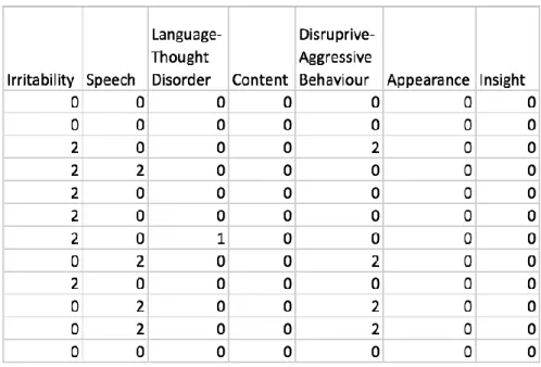
Figure 4.6. Fragment of the YMRS patient data (Part 2)
4.1.3. HDRS data set
Another scale that was used, the Hamilton Depression Rating Scale (HDRS) [19], is the most widely used scale for depression rating. It was designed to be completed after a clinical interview. It has different versions, that include more or less rating items. For this project, we used the HDRS17, as seen on Figure 4.7 and Figure 4.8, which has 17 different items regarding depression symptoms experienced by the patients in the previous week. These 17 items and their possible values are the following:
• Depressed Mood:
▪ 0: absent
▪ 1: feeling state indicated only on questioning
▪ 2: feeling state spontaneously reported verbally
▪ 3: communicates feeling state non-verbally (i.e. voice)
▪ 4: reports feelings only on spontaneous verbal and non-verbal behaviour • Feelings of guilt:
▪ 0: absent
▪ 1: feels that he or she has let people down
▪ 2: ideas of guilt
▪ 3: delusions of guilt
▪ 4: hears accusatory voices and experiences threatening hallucinations • Suicide:
▪ 0: absent
▪ 1: feels life is not worth living
▪ 2: wishes he or she was dead
▪ 3: ideas of suicide
28 • Insomnia (early in the night):
▪ 0: no difficulty falling asleep
▪ 1: occasional difficulty falling asleep
▪ 2: nightly difficulty falling asleep • Insomnia (middle of the night):
▪ 0: no difficulty
▪ 1: restless and disturbed during night
▪ 2: waking up during night
• Insomnia (early hours of the morning):
▪ 0: no difficulty
▪ 1: waking in early hours of the morning, goes back to sleep
▪ 2: unable to fall asleep again if he/she wakes up • Work and activities:
▪ 0: no difficulty
▪ 1: feelings of incapacity
▪ 2: loss of interest in activity
▪ 3: decrease in time spent (less than 3 hours) or productivity
▪ 4: stopped working because of illness • Retardation:
▪ 0: normal speech and thought
▪ 1: slight retardation during interview
▪ 2: obvious retardation during interview
▪ 3: interview difficult
▪ 4: complete stupor • Agitation:
▪ 0: none
▪ 1: fidgeting
▪ 2: playing with hands, hair, etc.
▪ 3: can’t sit still
▪ 4: nail biting, hair-pulling, etc. • Psychic anxiety:
▪ 0: no difficulty
▪ 1: subjective tension
▪ 2: worrying about minor matters
▪ 3: anxious attitude (apparent in face or speech)
29
• Somatic (physiological) anxiety (gastro-intestinal, cardio-vascular, respiratory, urinary frequency, sweating):
▪ 0: absent
▪ 1: mild
▪ 2: moderate
▪ 3: severe
▪ 4: incapacitating
• Somatic symptoms (gastro-intestinal):
▪ 0: none
▪ 1: loss of appetite but eating.
▪ 2: difficulty eating without staff urging • General somatic symptoms:
▪ 0: none
▪ 1: heaviness in limbs, back or head
▪ 2: clear-cut symptoms
• Genital symptoms (loss of libido, menstrual disturbances):
▪ 0: absent ▪ 1: mild ▪ 2: severe • Hypochondriasis: ▪ 0: not present ▪ 1: self-absorption
▪ 2: preoccupation with health
▪ 3: frequent complaints
▪ 4: hypochondriacal delusions • Loss of weight:
▪ According to patient: o 0: no weight loss
o 1: probable weight loss associated with illness o 2: definite weight loss
o 3: not estimated
▪ According to weekly measurements:
o 0: less than 1 lb (450g) loss in one week o 1: more than 1 lb (450g) loss in one week o 2: more than 2 lb (900g) loss in one week o 3: not estimated
• Insight:
▪ 0: acknowledges being depressed and ill
▪ 1: acknowledges illness but attributes it to other factors
30
Figure 4.7. Fragment of the HDRS patient data (Part 1)
Figure 4.8. Fragment of the HDRS patient data (Part 2)
4.1.4. Interview data set
The next file included data that had been gathered in interviews performed by the psychiatrist on different medical appointments with the patients, as seen in Figure 4.9 and Figure 4.10.
It contained both physical and psychological items. The psychological items represent more subjective data, like anxiety, irritability or concentration problems, whereas the physical items include more objective data, like the number of cigarettes that the patient has smoked in a day or the time in which the patient woke up or went to bed. The features used in the interviews were the following:
• Mood: mood level of the patient, ranging from -3 to 3.
• Motivation: motivation level of the patient, ranging from -3 to 3.
• Attention and concentration problems: level of attention and concentration problems of the patient, ranging from 0 to 4.
31
• Anxiety: anxiety level of the patient, ranging from 0 to 4.
• Sleep quality: quality level of the patient’s sleep, ranging from 0 to 4. • Menstrual cycle: whether a female patient is in her menstrual cycle.
• Number of cigarettes: number of cigarettes smoked by the patient since he or she woke up.
• Caffeine: amount of caffeine ingested by the patient since he or she woke up. • Alcohol: whether the patient has consumed any alcohol.
• Other drugs: whether the patient has consumed any other drugs. • Wake up time: when the patient woke up.
• Going to bed time: when the patient went to bed. • Code: patient code (first letter of the patient’s name). • Date: when the questionnaire was completed.
Figure 4.9. Interview data (Part 1)
32 4.1.5. Intervention data set
The last file included a summary of all the medical interventions that different doctors had with the patients, as shown in Figure 4.11. These interventions include medical appointments, videos, phone calls and interventions at Brief Hospitalization Units (UHB in the data frame) which are hospitalization units that provide a safe environment to resolve the disorder that has caused the need for urgent care in the shortest time possible. It also contains a value for the GAF (Global Assessment of Functioning) which evaluates symptoms, normal activities and interpersonal relationships of the patient.
Figure 4.11. Medical interventions
4.2.
Preparing the data
This part included the whole process of preparing the data to get clean data sets that could be used later for visualization and for algorithm training. Each data set was cleaned separately because they all had a different structure and size.
4.2.1. Episode data set
We started by giving the columns proper names so that all the data sets had a similar format (see Figure 4.12).
episodes.columns = ['patient', 'start', 'end', 'episode'] Figure 4.12. Column name translation of the Episode data set
The episodes that the patients had gone through were recorded as DEPRESIÓN and MANIA, which means depression and mania respectively. In order to make the data set cleaner, we changed the codes to D for depression and M for mania.
The dates presented in the data set were recorded in string format so, in order to have all the dates in the same format, we changed them to datetime, which is a Python module for manipulating dates. We iterated over every entry in the data set and changed the date, as seen in Figure 4.13.
33 for index, row in episodes.iterrows():
episodes['start'][index] = datetime.strptime(row.start, '%d/%m/%Y') episodes['end'][index] = datetime.strptime(row.end, '%d/%m/%Y')
Figure 4.13. Formatting the dates in the Episode data set
4.2.2. YMRS data set
The YMRS data set had a column named Observaciones that was filled with NaN (Not a Number) values. It didn’t add any value to the data set, so we dropped it (see Figure 4.14).
young = young.drop("Observaciones", 1)
Figure 4.14. Dropping Observaciones column from the YMRS data set
The next step was to rename the columns the same way as we did with the Episode data set (see Figure 4.15), so that we had all the names in the same format.
young.columns = [
'code', 'date', 'euphoria', 'hyperactivity', 'sexual_impulse', 'sleep', 'irritability', 'verbal_expression', 'language', 'thought', 'aggressiveness', 'appearance', 'illness_awareness'
]
Figure 4.15. Column name translation of the YMRS data set
We also needed to check if there were any empty (null) values in the data set, which we did with the Pandas isnull() function. After confirming that there were no empty values, we converted the dates in the data set to datetime format, like we did with the Episode data set.
4.2.3. HDRS data set
With this data set, we started by dropping the column Tipo de intervención the same way as we did with the YMRS data set, because it only had NaN values. We also renamed all the columns (see Figure 4.16) like we did with the previous data sets.
hamilton.columns = [
'code', 'date', 'depressed_mood', 'guilt', 'suicide', 'precocious_insomnia', 'medium_insomnia',
'verbal_expression', 'language', 'thought', 'late_insomnia', 'work', 'retardation', 'agitation', 'psychic_anxiety', 'somatic_anxiety',
'somatic_gastrointestinal_symptoms','somatic_general_symptoms ','genital_symptoms', 'hypochondria', 'weight_loss',
'illness_awareness' ]
Figure 4.16. Column name translation of the HDRS data set
With the isnull() function we obtained that there were empty values in the data set. We proceeded to print the values that were null. By printing the values of the rows before and after these empty values, we could get an idea of which values we could fill them with, which in this case was the same for all. So, we proceeded to fill the empty values with the ones obtained from these rows, as seen in Figure 4.17.
34
print(hamilton[hamilton.isnull().any(axis=1)][null_columns].head()) retardation agitation illness_awareness
0 NaN 0.0 0.0 3 0.0 0.0 NaN 14 0.0 NaN 0.0 print hamilton.at[1, 'retardation']
0.0
print hamilton.at[2, 'illness_awareness'] print hamilton.at[4, 'illness_awareness'] 0.0
0.0
print hamilton.at[13, 'agitation'] print hamilton.at[15, 'agitation'] 0.0
0.0
hamilton = hamilton.set_value(0, 'retardation', 0.0) hamilton = hamilton.set_value(3, 'illness_awareness', 0.0) hamilton = hamilton.set_value(14, 'agitation', 0.0)
Figure 4.17. Filling empty values in the HDRS data set
The next step was to format all the values in the data set so that they had the same type, because some values had Floating Point type and others had Integer type. We changed all to Integer. After that, just as we did with the Episode and YMRSdata sets, we changed the format of the dates to datetime.
4.2.4. Interview data set
The data set that contained the interview data from different medical appointments was the one that had the biggest amount of data and therefore presented a bigger challenge when cleaning it. The first step was to rename the columns, as we did with the other data sets (see Figure 4.18).
interviews.columns = [
'mood', 'motivation', 'attention', 'irritability', 'anxiety', 'sleep_quality', 'menstrual_cycle', 'nr_cigarettes',
'caffeine', 'alcohol', 'other_drugs', 'wake up time', 'going to bed time','patient', 'date'
]
Figure 4.18. Column name translation of the Interview data set
The next step was to unify the qualitative values (NO and SI) and map them (see Figure 4.19)giving them a numerical value (0 and 1).
35
interviews = interviews.replace(to_replace="NO", value="No")
interviews = interviews.replace(to_replace="SI", value="Si")
interviews = interviews.replace(to_replace="No", value=0) interviews = interviews.replace(to_replace="Si", value=1) Figure 4.19. Categorical value unification and mapping in the Interview data set
As the sleeping time overlapped different days (for example, the patients might have slept from 10 pm one day to 9 am the day after), it was easier to know how many hours the patient had been active instead of the hours of sleep. If the patient had gone to bed after midnight, we had to add 24 hours in order to get the correct amount of time that the patient had been active.
Before we could calculate the active time, we had to format the time stamps by removing the colons, so that we could compare different hours. This whole process can be seen in Figure 4.20.
interviews = interviews.replace(to_replace=":", value="")
interviews['wake up time'] = interviews['wake up time'].str.replace(':','') interviews['going to bed time'] =
interviews['going to bed time'].str.replace(':','')
interviews = interviews.apply(pd.to_numeric, errors='ignore') interviews.loc[
interviews['going to bed time'] <
interviews['wake up time'], 'going to bed time' ] = interviews['going to bed time'] + 2400
interviews['active_time'] =
abs((interviews['wake up time'] –
interviews['going to bed time']).astype(int))
Figure 4.20. Calculating the amount of active time in the Interview data set
After calculating the amount of active time, we could drop the Wake up time and Going to bed time columns as they were no longer relevant. The next step was to see if there were any empty values in the data set, which in this case was true. We could observe that the menstrual_cycle feature was empty in all rows, probably because all the patients in the study were males. The whole column was dropped because it didn’t add any value to the data set.
We needed to print the rest of the empty values in order to see if we could fill them with other data. We compared the irritability value that was empty with the previous value and the one after it to see if they were similar. We could see that both were 1, so we filled the empty space with that value. The other value that was missing was a date, which would most surely be between two other days, so we set the value to the missing day between them. This whole process can be seen in Figure 4.21.
36
null_columns=interviews.columns[interviews.isnull().any()] interviews[null_columns].isnull().sum()
irritability 1 menstrual_cycle 647 date 1 dtype: int64
interviews = interviews.drop("menstrual_cycle", 1)
null_columns=interviews.columns[interviews.isnull().any()] print(interviews[interviews.isnull().any(axis=1)][null_columns]) irritability date
306 NaN 19/08/2017 533 1.0 NaN
print interviews.at[305, 'irritability'] print interviews.at[307, 'irritability'] 1.0
1.0
interviews = interviews.set_value(306, 'irritability', 1.0) print interviews.at[532, 'date']
print interviews.at[534, 'date'] 03/07/2017
05/07/2017
interviews = interviews.set_value(533, 'date',
str('04/07/2017'))
Figure 4.21. Completing missing values in the Interview data set
After filling the empty values, we changed all the Floating Pointvalues to Integer and changed the dates to datetime, like we did with the rest of the data sets, in order to have the same format for all the numeric features and the dates.
4.2.5. Intervention data set
The first step in cleaning the intervention data set was to rename the columns, which we did with the other data sets (see Figure 4.22).
interventions.columns = [
'code', 'doctor', 'type', 'attends', 'date', 'gaf', 'relief' ]
Figure 4.22. Column name translation of the Intervention data set
We could also drop the rows that contained GAF values that were NaN, because we did not want to risk making up such concrete values. The doctor and the interventiontype were also dropped because they did not add any value to the data set and we wanted generic data.
37
The interventions that the patients did not attend to were not valuable either, so we dropped them from the data set (see Figure 4.23). This meant that we could get rid of the column that indicated if the patient attended or not, because at that moment we only had data from interventions that the patients had attended to.
interventions = interventions[interventions['attends'] != 'no'] Figure 4.23. Dropping entries from interventions that patients did not attend to
We only needed the numerical value of the column that indicated the relief felt by the patients on each intervention, so we split the strings and took only the number (see Figure 4.24), which ranged from 1 to 7 (1 being much better and 7 being much worse).
for index, row in interventions.iterrows(): splits = row.relief.split('.')
interventions['relief'][index] = splits[0] Figure 4.24. Taking the numerical value from the relief column
The only thing left was to change the date to datetime format, the same way as we did with the other data sets, in order to obtain a clean dataset.
38
5.
Exploratory Data Analysis
The Exploratory Data Analysis [20] is the process by which the data are visualized an analysed with the purpose of making sense of the data. This is fundamental in order to see how the data behave. With the help of different graphs and maps we could get a better understanding of all the data sets as well as the different combinations of them. The episode data set was not necessary to plot because it did not contain any numerical data, only periods of time.
In this part, we plotted each data set separately. Also, before plotting, we removed the date and code/patient columns which could not be plotted. It was also important to know which variables had more than one value in the data sets, because singular matrices cannot be plotted. For this, we made a function that showed which variables could be plotted in a data set (see Figure 5.1).
def get_plottable_columns(df): for column in df:
print column, ": ",
n_values = len(df[column].unique()) if n_values > 1:
print "Yes, ", n_values, " values" else:
print "No, 1 value"
Figure 5.1. Function that returns variables in a data set that can be plotted
For each data set, we used three types of visualization techniques:
• Histograms: this kind of plot gives a good overview on how the data are distributed in a data set, although it depends on the bins that are chosen, which are the intervals in which the data are classified into. This might not always be the best way to represent the data, as the whole of the data set is not plotted. • Heatmaps: these are graphs that show the correlation between all the features
in a data set, with a colour scale that represents a higher or lower correlation between the features.
• Scatterplots: this technique is very useful for studying the relationship between different features in a data set, showing a distribution of all the values of each feature. In this part, we included also the kernel density plots, which are quite useful to avoid overplotting, as they show where the values are more concentrated with different colour scales, and the marginal plots, which show both the distribution and the relationship between the features.
5.1.
YMRS data set
5.1.1.
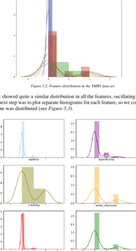
HistogramsThe first histogram we plotted was the one where we could see all the features distributed together, as seen in Figure 5.2.
39
Figure 5.2. Feature distribution in the YMRS data set
This plot showed quite a similar distribution in all the features, oscillating between -1 and 3. The next step was to plot separate histograms for each feature, so we could observe how each one was distributed (see Figure 5.3).