Methods for Addressing Data Diversity in Automatic Speech Recognition

(1)

Sheffield

The

University

Of

Methods for Addressing Data

Diversity in Automatic

Speech Recognition

Mortaza Doulaty Bashkand

Machine Intelligence for Natural Interfaces (MINI) Lab, Speech and Hearing (SPandH) Research Group,

Department of Computer Science, University of Sheffield

This dissertation is submitted on January 2017 for the degree of Doctor of Philosophy

(2)

(3)

“Everything not saved will be lost.” –Nintendo “Quite Screen” message

(4)

(5)

Abstract

The performance of speech recognition systems is known to degrade in mismatched conditions, where the acoustic environment and the speaker population significantly differ between the training and target test data. Performance degradation due to the mismatch is widely reported in the literature, particularly for diverse datasets.

This thesis approaches the mismatch problem in diverse datasets with various strategies including data refinement, variability modelling and speech recognition model adaptation. These strategies are realised in six novel contributions.

The first contribution is a data subset selection technique using likelihood ratio derived from a target test set quantifying mismatch. The second contribution is a multi-style training method using data augmentation. The existing training data is augmented using a distribution of variabilities learnt from a target dataset, resulting in a matched set.

The third contribution is a new approach for genre identification in diverse media data with the aim of reducing the mismatch in an adaptation framework.

The fourth contribution is a novel method which performs an unsupervised do-main discovery using latent Dirichlet allocation. Since the latent dodo-mains have a high correlation with some subjective meta-data tags, such as genre labels of media data, features derived from the latent domains are successfully applied to the genre and broadcast show identification tasks.

The fifth contribution extends the latent modelling technique for acoustic model adaptation, where latent-domain specific models are adapted from a base model. As the sixth contribution, an alternative adaptation approach is proposed where subspace adaptation of deep neural network acoustic models is performed using the proposed latent-domain aware training procedure.

All of the proposed techniques for mismatch reduction are verified using diverse datasets. Using data selection, data augmentation and latent-domain model adapta-tion methods the mismatch between training and testing condiadapta-tions of diverse ASR systems are reduced, resulting in more robust speech recognition systems.

(6)

(7)

Declaration

This dissertation is my own work and contains nothing which is the outcome of work done in collaboration with others, except where specified in the text. This dissertation is not substantially the same as any that I have submitted for a degree or diploma or other qualification at any other university. This dissertation does not exceed the prescribed limit of 80 000 words.

Mortaza Doulaty Bashkand January 2017

(8)

(9)

Acknowledgements

I would like to express my sincere gratitude to my supervisor, Prof. Thomas Hain. Without his continuous support and endless guidance this thesis would not have been possible.

I would also like to thank Oscar Saz and Raymond W. M. Ng for their kind support and the useful discussions we had throughout my PhD. The current and past members of the MINI group were all very helpful during my studies and I thank them all.

I wish to thank Richard Rose and Olivier Siohan of Google Inc. New York for having me as an intern in summer 2015.

My PhD was supported by the Engineering and Physical Sciences Research Coun-cil (EPSRC) programme grant EP/I031022/1 Natural Speech Technology (NST). I am grateful to the NST and EPSRC for the studentship they provided to fund my PhD research and to the Department of Computer Science of the University of Sheffield for funding the overseas element of the tuition fees.

I had a wonderful time during lunch breaks everyday chatting, watching videos and discussing the latest world and technology news with Rosanna Milner and Salil Deena.

Last but not least, I would like to thank my mother and deceased father for their unconditional support and devotion to their son. My deepest appreciation goes to my partner, Fariba Yousefi. Her wholehearted support made my PhD life a lot easier.

(10)

(11)

List of Acronyms

AM Acoustic Model

ASR Automatic Speech Recognition

BBC British Broadcasting Corporation

BN Bottleneck

BP Back Propagation

CAT Cluster Adaptive Training

CD Context Dependent

CE Cross-Entropy

CHN Cepstral Histogram Normalisation

CI Context Independent

CMLLR Constrained Maximum Likelihood Linear Regression

CMN Cepstral Mean Normalisation

CMVN Cepstral Mean and Variance Normalisation

CRF Conditional Random Field

CTC Connectionst Temporal Classification

CTS Conversational Telephone Speech

CVN Cepstral Variance Normalisation

DAT Device Aware Training

DBN Deep Belief Network

(18)

EM Expectation Maximisation

fDLR Feature Discriminative Linear Regression

fMLLR Feature-space Maximum Likelihood Linear Regression

GD Gender Dependent

GMM Gaussian Mixture Model

HMM Hidden Markov Model

idf Inverse Document Frequency

IR Information Retrieval

iVector Identity Vector

KLD Kullback-Leibler Divergence

LDA Latent Dirichlet Allocation

LHN Linear Hidden Network

LIN Linear Input Network

LM Language Model

LON Linear Output Network

LSI Latent Semantic Indexing

MAP Maximum A Posteriori

MCMC Markov Chain Monte Carlo

MFCC Mel-Frequency Cepstral Coefficients

MGB Multi-Genre Broadcast

ML Maximum Likelihood

MLLR Maximum Likelihood Linear Regression

MMI Maximum Mutual Information

(19)

MTR Multistyle Training

NAT Noise Aware Training

oDLR Output-feature Discriminative Linear Regression

PCA Principle Component Analysis

PDF Probability Density Function

PLP Perceptual Linear Prediction

pSLI Probabilistic Latent Semantic Indexing

RNN Recurrent Neural Network

ROVER Recognizer Output Voting Error Reduction

SA Speaker Adaptive

SAT Speaker Adaptive Training

SD Speaker Dependent

SGD Stochastic Gradient Descent

SGMM Subspace Gaussian Mixture Model

SI Speaker Independent

SVD Singular Value Decomposition

SVM Support Vector Machine

tf Term Frequence

tf-idf Term Frequency - Inverser Document Frequency

VQ Vector Quantisation

VTLN Vocal Tract Length Normalisation

WER Word Error Rate

(20)

(21)

List of Figures

1.1 Dependencies of the chapters . . . 13

2.1 Linear input network architecture . . . 24

2.2 Linear output network architecture, before softmax weights . . . 25

2.3 Linear output network architecture, after softmax weights . . . 25

2.4 Cluster adaptive training . . . 28

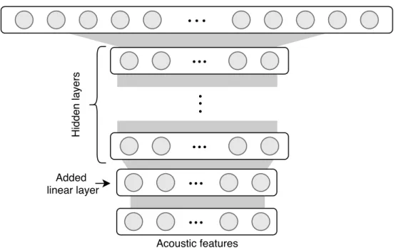
2.5 Subspace DNN architecture . . . 32

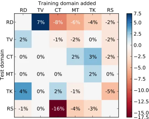
3.1 Heatmap of relative WER change by adding cross-domain data to in-domain models . . . 52

3.2 Relative WER (%) improvement with budget–based data selection . . 53

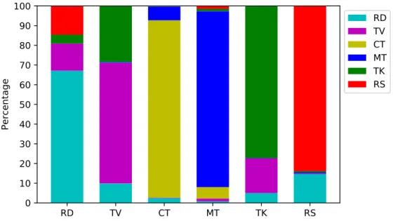
3.3 Types of data selected for a 10-hour budget using likelihood ratio similarity measure from the diverse dataset . . . 54

3.4 Impact of noise on phone posteriors for 10dB (top) and 25dB SNR (bottom) on the same 2 sec. utterance . . . 57

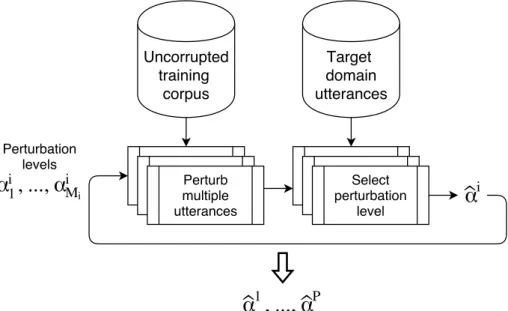
3.5 Perturbation level determination procedure . . . 60

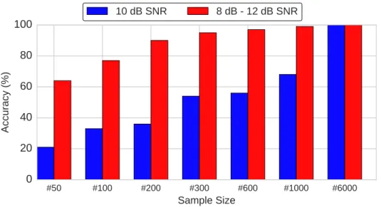
3.6 Classification accuracy of perturbation level over a range of dataset sample sizes . . . 61

3.7 Sequential estimation of perturbation levels for multiple perturbation types . . . 64

4.1 Asynchronous HMM topology with two environments . . . 74

4.2 Background tracking features extraction process . . . 76

4.3 One-minute samples of background tracking features for four different shows . . . 79

4.4 Genre classification accuracy (%) using GMMs, HMMs and SVMs on dataset A . . . 82

4.5 Graphical model representation of LDA . . . 85

4.6 Graphical model representation of the simplified distribution for the LDA model . . . 86

(22)

4.8 Acoustic LDA inference procedure . . . 91 4.9 Distribution of 133 shows in training and test set of dataset B . . . . 94 4.10 Distribution of the most important 16 LDA domains across genres . . 94 4.11 Distribution of the most important 16 LDA domains across different

episodes of two shows . . . 95

5.1 Amount of data for each discovered domain from the labelled domains 107 5.2 KL divergence of the training and test set latent domains . . . 108 5.3 WER (%) of LDA-MAP adapted models with different number of

latent domains . . . 109 5.4 Amount of data across LDA domains . . . 114 5.5 DNN architecture with LDaT . . . 115

(23)

List of Tables

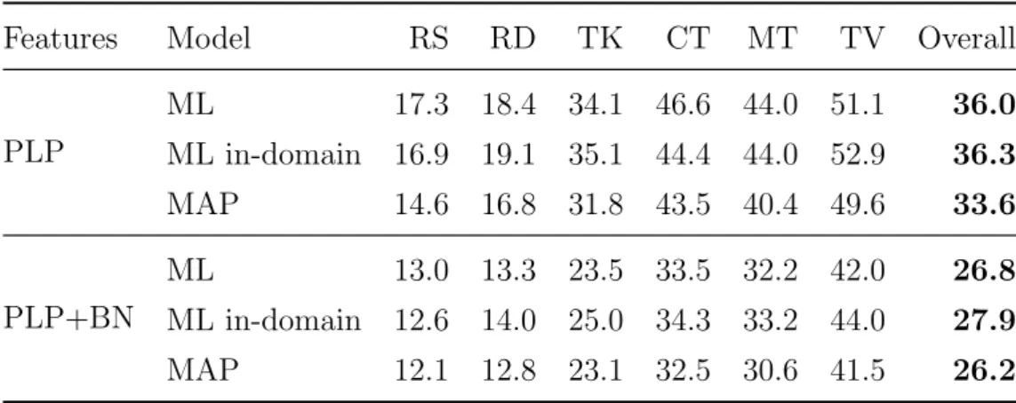
3.1 Training set statistics per component for the diverse dataset . . . 48 3.2 Test set statistics per component for the diverse dataset . . . 49 3.3 WER (%) of the baseline models on the test set of the diverse dataset 50 3.4 WER (%) on the test set of the diverse dataset using the

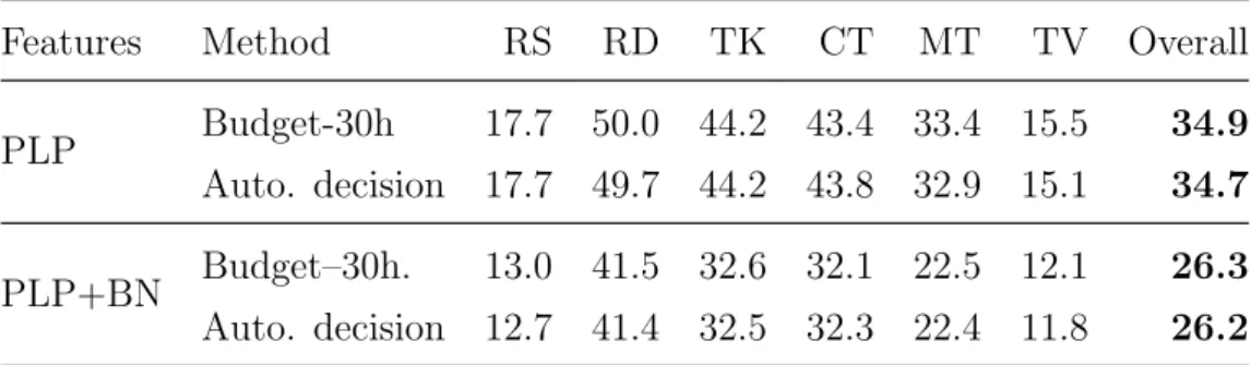
domain-specific models . . . 51 3.5 WER (%) of the baseline models with the diverse dataset . . . 55 3.6 Amount of data selected by the automatic budget decision . . . 55 3.7 WER (%) using MTR training scenarios . . . 67

4.1 Amount of training and test data per genre in dataset A . . . 77 4.2 Genre classification accuracy (%) with GMM models and short-term

PLP features on dataset A . . . 78 4.3 Genre classification accuracy (%) with GMM models and background

tracking features on dataset A . . . 80 4.4 Genre classification accuracy (%) using whole shows on dataset A . . 92 4.5 Amount of training and test data per genre for dataset B . . . 93 4.6 Genre/show classification accuracy (%) with GMMs on dataset B . . 96 4.7 Genre/show classification accuracy (%) using whole show and

seg-ment based acoustic LDA models on dataset B . . . 97 4.8 Genre/show classification accuracy (%) using text based LDA models

on dataset B . . . 99 4.9 Genre/show classification accuracy (%) using meta-data on dataset B 99 4.10 Genre/show classification accuracy (%) with system fusion on dataset B100

5.1 WER (%) of the baseline models on diverse dataset . . . 105 5.2 WER (%) of LDA-MAP models (K = 8) . . . 108 5.3 WER (%) of LDA-MAP models (K = 8) across hidden domains . . . 109 5.4 Amount of training and test data (hours) per genre for the MGB

dataset . . . 111 5.5 WER (%) of baseline BN models for the MGB dataset by genre . . . 111 5.6 WER (%) of LDA-MAP BN models for the MGB dataset per genre . 112

(24)

5.7 WER (%) of baseline hybrid models for the MGB dataset . . . 113 5.8 WER (%) of LDaT(+SAT) hybrid models for the MGB dataset . . . 116 5.9 Amount of training data for the Sheffield MGB system . . . 117 5.10 WER (%) on the MGB dataset using the two training sets . . . 117 5.11 WER (%) on the MGB dataset using domain and noise adaptation

with hybrid and bottleneck systems . . . 118 5.12 WER (%) of the different components of the Sheffield MGB 15 system

on the MGB dataset . . . 119

(25)

CHAPTER

1 Introduction

Automatic speech recognition (ASR) is the task of transcribing spoken language into text. It has a very wide range of applications, including but not limited to: voice dictation, voice command and control, home automation, personal assistants, au-tomatic translation, language learning, hands-free computing, auau-tomatic subtitling, interactive voice responders and medical reporting. As this technology improves and produces fewer errors, its application domain extends.

ASR can be considered as a mapping function that maps a variable length acous-tic signal into a variable length sequence of words:

f(O) = W (1.1)

whereO is an acoustic signal andW is the sequence of words spoken in the acoustic signal. Statistical approaches can be used for solving this problem and the mapping function can be defined in a probabilistic way:

ˆ

W = arg max

W∈L

P(W|O) (1.2)

this changes the ASR problem to a search problem: finding the most likely sequence of words from all of the possible word sequences of language L given the acoustic signal. Applying Bayes’ theorem to equation 1.2 yields:

ˆ W = arg max W∈L P(O|W)P(W) P(O) = arg maxW∈L P(O|W)P(W) (1.3)

where P(O|W) is the observation likelihood computed by an acoustic model (AM) and P(W) is the prior probability of the word sequence computed by a language model (LM). Since the probability of the observation itself, P(O), is independent from the most likely word sequence, it can be omitted from the search. The reason for

(26)

using the Bayes’ theorem is that the probabilities on the left-hand side of equation 1.3 is not directly computable.

Finding the most likely sequence of words, ˆW, is called decoding. The Viterbi algorithm (Viterbi, 1967) is usually used for decoding and during the search, scores from the AM and LM are combined together. For practical reasons and to speed up the search process, parts of the search space are usually pruned.

To assess performance of ASR systems, word error rate (WER) is the commonly applied metric. It is based on the minimum edit distance between the output of the ASR system and the reference text. The error is computed as the ratio between the total count of insertions, deletions and substitutions required to convert the hypothesised text to the reference text vs. total number of words in the reference text.

1.1 Acoustic and language modelling

1.1.1 Acoustic modelling

The observation sequence is usually sampled into frames. These frames are then transformed into some form of spectral representation such as Mel-frequency cepstral coefficients (MFCC) features. The AM is then used to compute the likelihood of the feature vectors given some linguistic units. There are several approaches for acoustic modelling and two of the most popular approaches will be introduced briefly in this section.

Using a lexicon each word can be represented as a sequence of sub-word units, such as phones. Usually these sub-word units are modelled with five-state hid-den Markov models (HMM) where the first and last states are non-emitting states which are used for concatenating these units. Considering the coarticulation effect, where each phone is pronounced differently depending on the neighbouring phones, in modern ASR systems context-dependent (CD) phones are modelled instead of context-independent (CI) phones. Since there are exponentially more CD phones compared to CI phones, and not all phone combinations are seen in the training data or sometimes not even possible at all, the HMM states of the CD phones are tied together for parameter sharing.

Gaussian mixture models (GMM), deep neural networks (DNN), support vector machines (SVM) or conditional random fields (CRF) can be used to model the probability density function (PDF) of emitting states of the HMMs (Jurafsky and Martin, 2000). Prior to 2012, GMMs were very popular for modelling the PDFs in acoustic modelling. With the raise of deep learning in 2012, several studies showed

(27)

that DNNs can be used to further improve acoustic modelling (Hinton et al., 2012; Yu and Deng, 2015).

With GMMs, each HMM state is usually modelled with an 8–64 component mixture model. Parameters of the model (including GMM weights, means and co-variances and HMM state transition probabilities) are learnt using the Baum-Welch algorithm. It uses the expectation maximisation (EM) algorithm to find the maximum likelihood (ML) estimate of the model parameters given the observation vectors.

To train the acoustic models the transcripts of the speech segments are commonly provided at the word level, however the modelling is performed on sub-word units such as phones. Usually a uniform distribution of the phones in the utterance is assumed and the initial models are trained with this initial alignment. Then, these models are used to acquire better state-level alignments and re-train more accurate models.

Initial proposals to use neural networks in HMM-based speech recognisers date back to the early 90’s (Renals et al., 1994). However, the success of those early attempts were not comparable to the state-of-the-art GMM-HMM systems. Around 2012, neural networks became popular again and several studies promoted the use of deep neural networks in speech recognition with some promising results. This was mostly because of having more computation power and more data available. It was shown that the use of DNNs could reduce the WER around 15–25% relative compared to the conventional GMM-HMM systems (Hinton et al., 2012; Yu and Deng, 2015).

There are two popular approaches to integrate DNNs with HMM-based speech recognition systems: bottleneck and hybrid setups (Gr´ezl et al., 2007; Renals et al., 1994). In both setups, a DNN is trained for classifying the frames into phone classes or tied HMM states of the CD phones. The state level alignment for training these DNNs is usually acquired by an initial GMM-HMM system.

In the bottleneck setup, the DNN acts as a feature extractor for the GMM-HMM system. Usually a bottleneck layer, which has a smaller number of neurons compared to other layers, is used in the neural network and outputs of the neurons from the bottleneck layer (either before or after the activation function) are used as a new representation of the input frames. These features are then used in a conventional GMM-HMM system as input features (either in solo mode or by augmenting the existing MFCC features).

With hybrid systems, GMMs are replaced by DNNs. In this setup, emissions of the HMM states are modelled by DNNs. Since HMM-based speech recognition systems require the likelihood computation and DNNs output posterior probabilities,

(28)

these scores are converted to likelihood scores using Bayes’ theorem.

An alternative approach for solving the speech recognition problem is the so-called end-to-end systems. Unlike phonetic-based systems where different compo-nents such as the AM, LM and lexicon are trained separately, the end-to-end tech-niques try to learn all of the components jointly. One of the first attempts was the connectionist temporal classification (CTC) approach proposed by Graves et al. (2006) which used recurrent neural networks (RNN) and CTC objective function to jointly learn the lexicon and AM without any explicit frame-level alignment. Other approaches also tried to map the acoustic signal directly to characters or even words (Bahdanau et al., 2016; Chan et al., 2016).

The scope of this thesis will be limited to HMM-based speech recognition systems and the ASR related contributions will be evaluated using DNN-based acoustic models.

1.1.2 Language modelling

In equation 1.3,P(W) is the prior probability of the word sequence which is modelled by a language model. N-grams are a simple form of count-based LMs and can be used to assign a probability to a word sequence or find the conditional probability of the next word given a history ofn−1 words. They are widely used in ASR, hand writing recognition and machine translation.

With advances in deep learning, neural network based LMs are outperforming n-grams in many tasks and will most likely replace them (Mikolov et al., 2010). More specifically, neural networks with recurrent units have better modelling capabilities for language modelling compared to feed-forward networks and most of the state-of-the-art LMs are based on RNNs (Mikolov et al., 2011). Since the focus of this thesis will be on acoustic modelling, LMs will not be studied in depth.

1.2 Motivation

Training acoustic models is usually considered as a supervised learning task which requires labelled training data. Speech data has various characteristics such as type of speech (fluent, natural and conversational), acoustic environment (noisy vs. clean), accent of the speakers, etc. These characteristics vaguely define the conven-tional domains in ASR (Deng and Li, 2013). However, the concept of a domain is complex and not bound to specific criteria. Training AMs from utterances that match the target speaker population, speaking style or acoustic environment is gen-erally considered to be the easiest way to optimise ASR performance. Furthermore, speech recognition performance is known to degrade when the acoustic environment

(29)

and the speaker population in the target utterances are significantly different from the conditions represented in the training data. However, the matched ASR systems usually require in-domain data, e.g. data which has the same underlying distribution as the target domain data. Mismatch happens when the underlying distributions of the training and test data are not the same and depending on level of mismatch, performance of the ASR systems can degrade significantly.

There are several approaches to address the mismatch problem in different lev-els of the ASR training process. One approach is to create a matched training set to a target test set and train ASR systems with the matched training set. For creating a matched set, often similarity measures are used and data selection is performed based on maximising the similarity measure. The training set can be selected from a fixed set of utterances, where the mismatch minimisation problem turns into a data subset selection problem. The objective in the data subset selec-tion problem is to select a subset of utterances from a pool of available utterances that matches a target set. If the pool of utterances can be extended by generating new samples or augmenting existing samples, then this problem turns into a data generation/augmentation problem. With this approach the training set can be ex-tended by various data generation and augmentation techniques to create a matched training set for a target test set.

With data selection/augmentation techniques, the task is to select/augment the existing data for training the models from scratch. In the case of having some already trained and possibly mismatched models, an alternative approach is to update the model parameters to better match the target test set. This mismatch minimisation technique is typically called model adaptation.

Reducing the mismatch typically improves the performance of ASR systems and the main motivation of this thesis is to study how different techniques can be used to reduce the mismatch between training and test conditions. For this purpose new techniques for data selection and augmentation are proposed. Furthermore, new representations of acoustic variability present in speech data are proposed which uses latent modelling techniques. These latent representations are then used for mismatch reduction of the ASR models.

In summary, this thesis studies various different techniques for minimising the mismatch between training and testing conditions in diverse datasets with the ulti-mate aim of improving performance of the ASR systems.

1.3 Contributions

(30)

1. data selection based on similarity to a target set: developing a new data selection algorithm based on similarity to a target set for mismatch min-imisation (chapter 3)

2. data augmentation based on the identified levels of variations: devel-oping a new algorithm for learning the distributions of variations present in a target set and augmenting the training data with the learnt distribution for mismatch minimisation (chapter 3)

3. genre identification using background tracking features: identifying genres of media data using local background tracking features for improving the in-domain ASR systems (chapter 4)

4. genre and broadcast-show identification using latent Dirichlet allo-cation: identifying genres and broadcast-shows of media data using latent Dirichlet allocation-based features and investigating the required sources of information for reaching high levels of accuracy (chapter 4)

5. adaptation of acoustic models to latent domains: identifying latent domains in diverse datasets and adapting acoustic models to latent domains (chapter 5)

6. latent domain aware training of DNNs: organising broadcast media using latent modelling and adapting DNNs to the latent domains (chapter 5)

1.3.1 Data selection based on similarity to a target set

In this work the mismatch minimisation problem was studied as a data subset se-lection problem. The motivation of this study was to reduce the mismatch between training and test data by data selection techniques. Given a target test set and a pool of diverse training utterances, the task was to select a subset of training data such that the performance of the ASR system trained with this subset should be comparable to the model that is trained with all of the available data. The likeli-hood ratio was used to decide whether data resembels a target set. This approach was evaluated on a diverse dataset, covering speech from radio and TV broadcasts, telephone conversations, meetings, lectures and read speech. Experiments demon-strated that the proposed technique both finds the relevant data and limits the effects of negative transfer (negative transfer happens when the extra data affects the performance negatively). Results on a 6-hour test set showed relative WER improvements of up to 4% with the proposed data selection technique over using all of the available training data.

(31)

Relevant publication: Mortaza Doulaty, Oscar Saz, Thomas Hain, “Data-selective transfer learning for multi-domain speech recognition,” in Proceedings of Interspeech, Dresden, Germany, 2015.

1.3.2 Data augmentation based on the identified levels of

variations

The motivation of this work was to study how data augmentation techniques can be used for mismatch reduction. An alternative approach to address the mismatch problem is to augment the training data by perturbing the utterances in an existing uncorrupted and potentially mismatched training speech corpus to better match target test set utterances. An approach was proposed that, given a small set of utterances from a target test set, automatically identified an empirical distribution of perturbation levels that could be applied to utterances in an existing training set. Distributions were estimated for perturbation types that included acoustic back-ground environments, reverberant room configurations, and speaker related varia-tions such as frequency and temporal warping. The end goal was for the resulting perturbed training set to match the variabilities in the target domain and thereby optimise ASR performance. An experimental study was also performed to evaluate the impact of this approach on ASR performance when the target utterances were taken from a simulated far-field acoustic environment. Using the proposed approach, 10% relative improvement of the WER over the uniform perturbation baseline was achieved.

This work was performed during an internship of the author at Google Inc., New York. The original idea of this internship project was proposed by Richard Rose and Olivier Siohan and all of the follow-up research, implementation and experimental work was performed by Mortaza Doulaty Bashkand with collaboration of his co-authors.

Relevant publication: Mortaza Doulaty, Richard Rose, Olivier Siohan, “Au-tomatic optimization of data perturbation distributions for multi-style training in speech recognition,” in Proceedings of IEEE Workshop on Spoken Language Tech-nology (SLT), San Diego, California, USA, 2016.

1.3.3 Genre identification using background tracking

fea-tures

Tagging diverse media data with labels such as genre has many applications in multimedia information retrieval systems. Since shows within the same genre share similar acoustic conditions, grouping media data based on such labels can be used

(32)

for data selection and model adaptation of ASR systems as well. This served as a motivation to study the genre identification task in more depth. In this work using a set of local features describing the most likely background environment for each frame, higher level concepts such as genres were identified. These local features were based on the output of an alignment that fits multiple asynchronous parallel background-based linear transformations to the input audio signal. These features can be used to keep track of changes in background conditions, such as presence of music, laughter, applause and etc. The proposed approach was tested on a set of 332 shows from the British Broadcasting Corporation (BBC). Using different classifiers such as HMMs and SVMs, an accuracy of 83% was achieved on this dataset.

Note that at the time of publishing this work, there were no external baselines available for comparison. Relevant baselines are provided in the corresponding sec-tion. Access to this data is available with a license agreement with the BBC.

The original asynchronous factorisation work was performed by Oscar Saz and the use of features derived from background indexes for the genre classification task was a joint work between Oscar Saz and Mortaza Doulaty Bashkand.

Relevant publication: Oscar Saz, Mortaza Doulaty, Thomas Hain, “Background-tracking acoustic features for genre identification of broadcast shows,” inProceedings of IEEE Workshop on Spoken Language Technology (SLT), Lake Tahoe, Nevada, USA, 2014.

1.3.4 Genre and show identification using latent Dirichlet

allocation

Since media data has a complex structure, acoustic latent Dirichlet allocation was proposed for modelling the media data. It was assumed that there was a set of latent factors that contributed to the generation of the media data and each show can be described as a mixture of those latent factors. Experiments were conducted on more than 1200 hours of TV broadcasts from the BBC, where the task was to categorise the broadcasts into 8 genres or 133 show identities. Furthermore, extra sources of information such as show transcripts and meta-data were studied for improving the classification performance. On a 200-hour test set, accuracies of 98.6% and 85.7% were achieved for genre and show identification respectively, using a combination of acoustic and textual features with meta-data.

Relevant publication: Mortaza Doulaty, Oscar Saz, Raymond W. M. Ng, Thomas Hain, “Automatic genre and show Identification of broadcast media,” in

(33)

1.3.5 Adaptation of acoustic models to latent domains

Posterior Dirichlet parameters from acoustic latent Dirichlet allocation (LDA) mod-els have discriminatory information and were successfully used for genre and show identification tasks. The motivation of this study was to explore how this informa-tion can be used for acoustic model adaptainforma-tion. In this work using a diverse dataset, a novel method to perform unsupervised discovery of latent domains using acous-tic LDA was proposed. A set of hidden domains was assumed to exist in the data, whereby each audio segment can be considered to be a weighted mixture of the latent domain properties. The classification of audio segments into latent domains allowed the creation of latent domain specific acoustic models. Experiments were conducted on a dataset of diverse speech data covering speech from radio and TV broadcasts, telephone conversations, meetings, lectures and read speech, with a joint training set of 60 hours and a test set of 6 hours. Maximum A Posteriori (MAP) adaptation to latent domains was shown to yield relative WER improvements of up to 10%, compared to the models adapted with human-labelled prior domain knowledge.

Relevant publication: Mortaza Doulaty, Oscar Saz, Thomas Hain, “Unsuper-vised domain discovery using latent Dirichlet allocation for acoustic modelling in speech recognition,” in Proceedings of Interspeech, Dresden, Germany, 2015.

1.3.6 Latent domain aware training of deep neural networks

It was shown that more latent domains were beneficial for the genre and show identification tasks. However, with the previous MAP adaptation approach the full potential of the acoustic LDA models could not be exploited, mostly because of data sparsity issues. This served as a motivation to study alternative approaches to incorporate acoustic LDA information for acoustic model adaptation. This work was focused on transcription of multi-genre broadcast media, which is often only categorised broadly in terms of high level genres such as sports, news, documentary, etc. However, in terms of acoustic modelling these categories are coarse. Instead, it is expected that a mixture of latent domains can better represent the complex and diverse behaviours within a TV show, and therefore lead to better and more robust performance. Using LDA modelling, these latent domains were identified and used to adapt DNNs using the one-hot vector representation of the LDA domains. Experiments were conducted on a set of BBC TV broadcasts, with more than 2,000 shows for training and 47 shows for testing. It was shown that latent domain aware training of the DNNs reduced the WER by up to 13% relative compared to the baseline hybrid DNN models.

(34)

(MGB) 15 system. The relevant LDA-DNN experiments were all conducted by Mortaza Doulaty Bashkand. Other models that were used for comparison and the overall Sheffield system were a joint work between the co-authors of the Sheffield MGB 15 system.

Relevant publication 1: Mortaza Doulaty, Oscar Saz, Raymond W. M. Ng, Thomas Hain, “Latent Dirichlet allocation based organisation of broadcast me-dia archives for deep neural network adaptation,” in Proceedings of IEEE Auto-matic Speech Recognition and Understanding Workshop (ASRU), Scottsdale, Ari-zona, USA, 2015.

Relevant publication 2 (for the Sheffield MGB 15 system): Oscar Saz, Mor-taza Doulaty, Salil Deena, Rosanna Milner, Raymond W. M. Ng, Madina Hasan, Yulan Liu, Thomas Hain, “The 2015 Sheffield system for transcription of multi-genre broadcast media,” inProceedings of IEEE Automatic Speech Recognition and Understanding Workshop (ASRU), Scottsdale, Arizona, USA, 2015.

1.4 Organisation

The remainder of this thesis is organised as follows: in chapter 2 a unified view of the domain mismatch problem will be defined and AM adaptation techniques will be reviewed. Chapter 3 will study data selection and augmentation techniques in the context of domain mismatch reduction. Chapter 4 will introduce two new techniques for identifying genre and show entities in the diverse datasets using local expert features. Chapter 5 is devoted to the study of incorporating latent domain representations of the speech data in the framework of acoustic model adaptation for mismatch reduction. Finally, chapter 6 provides a summary of this thesis and outlines the possible directions for future work.

To demonstrate how the chapters are related to each other, figure 1.1 presents dependencies between them. Chapter 2 and chapter 4 can be read directly, but reading chapter 3 requires reading chapter 2 first. Furthermore, chapter 2 and chapter 4 are the prerequisites for reading chapter 5.

1.5 Published work

This section lists the peer-reviewed and published papers during the PhD studies. The first six publications are already introduced in section 1.3 and contain the main contributions of this thesis. The remainder of the publications contain auxiliary

(35)

work related to this thesis.

1. Mortaza Doulaty, Oscar Saz, Thomas Hain, “Data-selective transfer learning for multi-domain speech recognition,” in Proceedings of Interspeech, Dresden, Germany, 2015.

2. Mortaza Doulaty, Oscar Saz, Thomas Hain, “Unsupervised domain discovery using latent Dirichlet allocation for acoustic modelling in speech recognition,” inProceedings of Interspeech, Dresden, Germany, 2015.

3. Mortaza Doulaty, Oscar Saz, Raymond W. M. Ng, Thomas Hain, “Latent Dirichlet allocation based organisation of broadcast media archives for deep neural network adaptation,” inProceedings of IEEE Automatic Speech Recog-nition and Understanding Workshop (ASRU), Scottsdale, Arizona, USA, 2015.

4. Mortaza Doulaty, Oscar Saz, Raymond W. M. Ng, Thomas Hain, “Automatic genre and show Identification of broadcast media,” in Proceedings of Inter-speech, San Francisco, California, USA, 2016.

5. Mortaza Doulaty, Richard Rose, Olivier Siohan, “Automatic optimization of data perturbation distributions for multi-style training in speech recognition,” inProceedings of IEEE Workshop on Spoken Language Technology (SLT), San Diego, California, USA, 2016.

6. Oscar Saz, Mortaza Doulaty, Thomas Hain, “Background-tracking acoustic features for genre identification of broadcast shows,” in Proceedings of IEEE Workshop on Spoken Language Technology (SLT), Lake Tahoe, Nevada, USA, 2014.

7. Oscar Saz, Mortaza Doulaty, Salil Deena, Rosanna Milner, Raymond W. M. Ng, Madina Hasan, Yulan Liu, Thomas Hain, “The 2015 Sheffield system for transcription of multi-genre broadcast media,” in Proceedings of IEEE Auto-matic Speech Recognition and Understanding Workshop (ASRU), Scottsdale, Arizona, USA, 2015.

8. Rosanna Milner, Oscar Saz, Salil Deena, Mortaza Doulaty, Raymond WM Ng, Thomas Hain, “The 2015 Sheffield system for longitudinal diarisation of broadcast media,” in Proceedings of IEEE Automatic Speech Recognition and Understanding Workshop (ASRU), Scottsdale, Arizona, USA, 2015.

9. Raymond W. M. Ng, Mortaza Doulaty, Rama Doddipatla, Wilker Aziz, Kashif Shah, Oscar Saz, Madina Hasan, Ghada AlHarbi, Lucia Specia, Thomas Hain,

(36)

“The USFD spoken language translation system for IWSLT 2014,” in Proceed-ings of International Workshop on Spoken Language Translation (IWSLT), Lake Tahoe, Nevada, USA, 2014.

10. Salil Deena, Madina Hasan, Mortaza Doulaty, Oscar Saz, Thomas Hain, “Com-bining feature and model-based adaptation of RNNLMs for multi-genre broad-cast speech recognition,” inProceedings of Interspeech, San Francisco, Califor-nia, USA, 2016.

11. Thomas Hain, Jeremy Christian, Oscar Saz, Salil Deena, Madina Hasan, Raymond WM Ng, Rosanna Milner, Mortaza Doulaty, Yulan Liu, “webASR 2 -improved cloud based speech technology,” in Proceedings of Interspeech, San Francisco, California, USA, 2016.

12. Raymond W. M. Ng, Mauro Nicolao, Oscar Saz, Madina Hasan, Bhusan Chet-tri, Mortaza Doulaty, Tan Lee, Thomas Hain, “The Sheffield language recog-nition system in NIST LRE 2015,” inProceedings of the Speaker and Language Recognition Workshop Odyssey, Bilbao, Spain, 2016.

13. Erfan Loweimi, Mortaza Doulaty, Jon Barker, Thomas Hain, “Long-term sta-tistical feature extraction from speech signal and its application in emotion recognition”, in Proceedings of International Conference on Statistical Lan-guage and Speech Processing (SLSP), Budapest, Hungary, 2015.

(37)

Ch1. Introduction

Ch2. Background

Ch3. Data selection and augmentation techniques

Ch4.

Identification of genres and shows in media data

Ch5.

Latent domain acoustic model adaptation

Ch6.

Conclusion and future work

(38)

(39)

CHAPTER

2 Background

2.1 Introduction

Often the term domain is used to vaguely define collections of speech data that share the same acoustic attributes and variabilities, such as type of speech (read vs. spontaneous), communication channel, background conditions and number of speakers. Conventional ASR domains often include broadcast news, meetings, tele-phony speech, audio books, lectures and talks (Benesty et al., 2007; Huang et al., 2001; Jurafsky and Martin, 2000). However, the concept of a domain is complex and not bound to specific criteria. In this section a new definition of a domain from a statistical point of view is provided based on the notations introduced in (Pan and Yang, 2010).

A domain is defined as a pair which consists of a feature space and a marginal probability distribution of data in that space:

D={X, P(X)} (2.1)

where X is a feature space, X = {x1, . . . , xn} ⊆ X is a dataset and P(X) is the

marginal probability distribution of the data in the feature space.With this notation two domains are different when either their feature spaces are different or they have different marginal probability distributions or both.

For the ASR task, X is the space of all arbitrary length segments of i.e. 39-dimensional MFCC feature vectors,Xis a training dataset andxi ∈Xis a particular

speech segment. The conventional domains in ASR such as meetings, read speech or talks can be considered to share the same feature space, but have different marginal probability distributions.

(40)

A task is defined as:

T ={Y, f()} (2.2)

where Y is a label space and f() is a prediction function which maps some input sequence to some output sequence:

f :X → Y. (2.3)

Two tasks are considered different when their label spaces are different or they have different prediction functions or both.

In supervised learning, the training data consists of (xi, yi) pairs such that f(xi) = yi and xi ∈ X, yi ∈ Y, Xtrn = {x1, . . . , xn} and Ytrn = {y1, . . . , yn}.

In a probabilistic learning framework, f() can be viewed as P(y|x), the posterior probability of the output,y, given the input,x. This function is usually not observed directly and learned from the training data.

In the speech recognition example, Y is the set of all possible sequences of words in English (defined as L in chapter 1) and f() is a mapping function which maps an audio segment to a sequence of words. Using the same audio signal for speech recognition and emotion identification (where the task is to identify the emotion of the speaker) can be considered as two different tasks, since the label space as well as the prediction functions are different, but both tasks share the same input to their prediction functions.

In many machine learning problems, the source and target domains (underlying distributions of the training and test data) are assumed to be the same: Dtrn =Dtst.

Furthermore the tasks are identical as well: Ttrn = Ttst. But in realistic scenarios

the domains are usually different and this causes mismatch between the training and test domains. The next section is devoted to the domain mismatch problem.

2.2 Domain mismatch

One of the key assumptions in many statistical approaches for machine learning problems is that the training and test data are drawn from the same underlying distribution (Hermansky et al., 2015; Pan and Yang, 2010). However, in practice this assumption is not always true and the mismatch in training and test data degrades the performance. Actually in practical scenarios even if the training and test data are drawn from the same underlying distributions, after the deployment of the models and over time the new test data will be inevitably different from the original training and test data and this will cause a mismatch in the model (Yu and Deng, 2015).

(41)

Domain mismatch happens when Dtrn 6=Dtst where Dtrn, Dtst are the training

and test domains respectively and it implies Xtrn 6=Xtst and/or Ptrn 6=Ptst (where Ptrn, Ptst are the marginal probability distributions of the training and test sets).

Domain adaptation aims at reducing the mismatch and is studied under different names in different fields. In econometrics it is called sample bias selection (Zadrozny, 2004), in statistical learning it is called covariate shift (Shimodaira, 2000), in machine learning it is called domain adaptation or transductive transfer learning (Arnold et al., 2007; Daume III and Marcu, 2006; Pan and Yang, 2010) and in the speech recognition community it is also called domain adaptation.

The performance of automatic speech recognition systems when applied to a particular domain depends on the degree to which the acoustic models provide an accurate representation of that domain. Training acoustic models from utterances that match the target speaker population, speaking style, acoustic environment, etc. (the factors that characterise the marginal probability distribution of the data in the feature space) is generally considered to be the easiest way to optimise the ASR performance. However, there are many scenarios where speech corpora of sufficient size that characterise the sources of variability existing in a particular target do-main are not available. For example, it has been shown that ASR performance in many applications benefits from using many thousands of hours of speech utterances collected from a similar domain (Jaitly et al., 2012). Having enough matched high quality training data is rarely a practical option and training ASR systems with mis-matched data results in poor performance. Adaptation techniques try to address these issues. Even if matched data exists, after deployment of the ASR systems new data will not be as good a match as it used to be before. This is mostly due to new environments, unseen speakers or even changes to voice of the current speakers over time (Yu and Deng, 2015). This further motivates the studies conducted in this thesis for mismatch compensation.

2.3 Relations to transfer learning

Adaptation techniques are a subset of a broader set of techniques in machine learning called transfer learning. Transfer learning aims to improve the performance of a machine learning algorithm using the knowledge acquired in a different domain or task (Pan and Yang, 2010). E.g. given a source and a target domain and their corresponding learning tasks: DS,DT,TS,TT, transfer learning aims to improve the

performance of the objective predictive function in the target task fT() using DS, TS where the source and target domains are different: DS 6= DT or the source and

(42)

The ideas behind transfer learning have very close resemblance to many natural and real-world problems. For humans, knowing how to drive a car is beneficial in learning how to drive a tractor. Humans are very good at transfer learning and most of the time they use this skill unconsciously and without any extra effort by leveraging some similar knowledge and skills they learned in the past (Pan and Yang, 2010).

2.3.1 Positive and negative transfer

The ultimate aim of transfer learning is to improve performance. When knowledge is transferred successfully and the performance is improved, it is called a positive transfer. However, in some cases it might happen that the transferred knowledge not only did not help to improve the performance, but also damaged it. When the transferred knowledge is harmful, the transfer is called a negative transfer. Measur-ing positive and negative transfer effects is usually trivial durMeasur-ing the model trainMeasur-ing phase, where labelled data is available for the evaluation. However, after deploy-ment of the model, it is not always easy to measure these effects on the new and unlabelled data.

In the literature the effects of negative transfer are not well studied (Pan and Yang, 2010). This served as a motivation to study the effects of negative transfer in the context of data selection for ASR in this thesis. The details of this study will be presented in chapter 3.

2.3.2 Transductive transfer learning

As discussed earlier, domain adaptation can be considered as a subset of transfer learning techniques. In the machine learning literature, a special term is used for this: transductive transfer learning (Arnold et al., 2007; Daume III and Marcu, 2006; Pan and Yang, 2010). A similar definition to transfer learning can be provided for transductive transfer learning: given a source and a target domain and their corresponding learning tasks: DS,DT,TS,TT, the aim is to improve the performance

of the objective predictive function in the target task fT() using DS, TS where the

source domains are different but tasks are the same: DS 6=DT orTS =TT.

This is equivalent to domain adaptation in speech recognition. An overview of adaptation techniques for ASR is provided in the next section.

(43)

2.4 Adaptation for mismatch compensation

As discussed in the previous sections, the mismatch between training and test data causes a degradation in performance of ASR systems. To compensate for the mis-match between training and test conditions, adaptation and normalisation tech-niques can be used. Adaptation techtech-niques are typically divided into model-based and feature-based techniques (Huang et al., 2001). The former, updates the model parameters to better fit the data and the later transforms the features to better fit the model.

The mismatch can be caused from various sources of variability, such as speaker or environment variabilities. In the ASR literature, mostly speaker variabilities are studied in the context of speaker adaptation where the aim is to compensate for the speaker variations. However, some speaker adaptation techniques can be used to compensate for other sources of variability, such as environment, device or the more generic notion of domain (Yu and Deng, 2015).

The conventional GMM-HMM based speaker dependent (SD) systems have a lower WER by a factor of two to three compared to speaker independent (SI) systems which are trained with similar amounts of data (Woodland, 2001). This demonstrates the impact of mismatch between the training and test conditions on the WER. On the other hand, it is not always easy to train SD systems, since they require a reasonable amount of transcribed data from the same speaker and the pro-cess of acquiring data and transcribing is time consuming and needs manual work in most cases (Cox, 1995; Woodland, 2001). So this makes speaker adaptive (SA) systems more interesting, as they fill the gap between the SD and SI systems. SI system are typically used to create a SA system.

The notion of dependency to speaker can be generalised to other intrinsic or extrinsic variabilities. For example if an ASR system for the South African English accent is to be trained, usually the best choice of training data would be from the same accent. However, if such training data is not available or only small amounts are available, then an accent independent system with the existing data can be trained and later it can be adapted to that specific accent.

Adaptation can be performed in different modes: it can be either supervised or unsupervised. It can also be in batch or incremental mode. In supervised adaptation, the correct transcription (word level) of the adaptation data is known. However, in case of unsupervised adaptation, the transcription for the adaptation data is a hypothesis which is generated by an ASR system. The problem with unsupervised adaptation is the quality of the estimated transcription which can make the system become even worse. Therefore, a confidence measure can be used to determine

(44)

the quality of the estimated transcription (Woodland, 2001; Yu, 2006; Zavaliagkos et al., 1998). With correct confidence measures, systems with even 80% WER can be improved (Zavaliagkos et al., 1998).

Adaptation can also be in either batch (static or block) or incremental (dynamic) mode. In batch adaptation the system is presented with the whole adaptation data before the final system is produced, however, in incremental mode the adaptation data is presented gradually and the system is adapted over the time (Yu, 2006). Depending on the application type, one can choose the most appropriate mode of adaptation (Kumar et al., 2013).

As introduced in chapter 2, the PDFs of the HMM-based acoustic models are often modelled by GMMs or DNNs. Various adaptation techniques are proposed for both techniques and a brief summary of them are provided in the next section.

2.5 Overview of acoustic model adaptation

tech-niques

Adaptation techniques can be categorised into these three main schemes (Woodland, 2001; Yu and Deng, 2015):

• transformation-based adaptation where model parameters or features are transformed using (linear) transformations learned from the adaptation data

• model re-training or conservative training where some of the model parameters (or all of them) are re-estimated from the adaptation data

• subspace adaptationwhere the model parameters are updated based on the representation of the adaptation data in some subspaces

2.5.1 Transformation-based adaptation

2.5.1.1 GMM-based acoustic models

The mismatch between training and test conditions can be minimised using a trans-form to alter the model parameters. In transtrans-formation-based approaches for adap-tation of GMM-based speech recognisers, model parameters including means and/or covariances of the Gaussian components can be transformed using a linear trans-formation to maximise the likelihood of the adaptation data, given the model. Es-pecially when the amount of adaptation data is limited and a fast adaptation is desired, linear transformation-based approaches are used (Gales and Young, 2008). Two types of linear transformations are introduced next.

(45)

Maximum likelihood linear regression

The ML criterion is typically used for training initial AMs where the likelihood of the training data given the model parameters and the correct transcription is maximised. ML estimation is defined as:

ˆ

λM L = arg max λ

p(O|W, λ) (2.4)

whereO is the training data, W is the correct transcription and λ is the parameter set.

The ML estimator can be used to learn a linear transform to maximise the likelihood of the adaptation data. Differences in speakers mostly affect the means of the feature vectors (Leggetter and Woodland, 1995) and thus, transforming the means would neutralise that effect. Means are transformed linearly using:

ˆ

µ=Wµ+b (2.5)

where W is a weight matrix and b is a bias vector.

Using the EM algorithm, a closed form solution to estimate W and b is de-rived (Leggetter and Woodland, 1995). One global transformation can be learned and applied to all of the Gaussian components, or different transformations for each subset of the Gaussian components can be learned and applied. Depending on the amount of available adaptation data a number of the transforms can be defined, e.g. for a few seconds of adaptation data, it is better to have a single transformation and as the amount of the adaptation data increases, more transformations can be used. This is achieved by grouping the Gaussian components together and learning a transform for each group. These groups are called base classes. Grouping Gaus-sian components can be performed in either a static or dynamic way (Gales and Young, 2008). A simple grouping can be performed based on the phonetic charac-teristics such as silence, vowels, stops, glides, nasals, fricatives, etc. (Young et al., 2006; Yu, 2006). One problem with the static methods is that since the number of groups are fixed and predefined, the amount of adaptation data does not change the number of these base classes and thus, all benefits of having more adaptation data is not exploited. However, dynamic methods can deal with adaptation data more efficiently and can have a variable number of groups depending on the availability of adaptation data. A simple dynamic grouping method can be based on the closeness of the Gaussian components in the acoustic space, e.g. centroid splitting algorithm with Euclidean distance (Young et al., 2006; Yu, 2006). This process is also called transformation sharing.

(46)

Covariance matrices can also be transformed. There are two alternative ways of transforming covariances: constrained MLLR and unconstrained MLLR (Shinoda, 2011). In the case of unconstrained MLLR, the variance is transformed using:

ˆ

Σ =LHLT (2.6)

where H is the Choleski factor of Σ, the original covariance matrix.

Mean adaptation is usually more effective than covariance adaptation and since the later is computationally expensive as well, mean adaptation is often preferred. Relative improvement of up to 15% with mean transformation is reported in the lit-erature for telephony speech, meetings and broadcast news (Woodland, 2001), while adapting covariance yields only 2% WER reduction for most of those tasks (Shinoda, 2011).

Constraint maximum likelihood linear regression

In the constraint maximum likelihood linear regression (CMLLR), the covariance matrix is transformed with the same transformation which is used to transform the means:

ˆ

µ=Wµ+b

ˆ

Σ = WTΣW. (2.7)

This can be considered as applying the transforms at the feature level:

ˆ

ot=W−1ot+b. (2.8)

When calculating the likelihood of the Gaussians, a factor |W| is required and expressed as:

N(O,µ,ˆ Σ) =ˆ |W| N(W−1O+W−1b;µ,Σ). (2.9)

Since the parameters of the model do not change in CMLLR, it becomes a good choice for situations where the speaker and acoustic environment change rapidly (Gales and Young, 2008).

CMLLR is also called feature-space maximum likelihood linear regression (fM-LLR).

2.5.1.2 DNN-based acoustic models

Similar to the transformation-based adaptation of the GMM-based acoustic mod-els, parameters of the DNN-based acoustic models can be updated using (linear) transformations.

(47)

In the following sections and also throughout the thesis, the following notation for DNNs will be used. v0_{is the input to the network (equivalent to}_o_{in the previous} notation), zi_, _vi _{are the output of} _i_{th layer before and after the activation function}

(called excitation and activation vectors respectively), Wi _and _bi _{are the weight}

matrix and bias vector of the layer i and f() is the activation function. With this notation, excitation and activation of theith layer are defined as:

zi =Wivi−1+bi, (2.10)

vi =f(zi). (2.11)

Transformation-based adaptation techniques are one of the most common adap-tation methods where a linear transformation is applied (by the means of an extra layer) to either input features (Abrash et al., 1995), input to the softmax layer (Li and Sim, 2010) or activation of the hidden layers (Gemello et al., 2007).

Linear input network

When the transformation is applied to the input layer, it is called linear input network (LIN) or feature discriminative linear regression (fDLR) (Seide et al., 2011). It assumes that the SD features can be linearly transformed to an average speaker’s features. For each speaker, a weight matrix and a bias vector is learned together with the other parameters using the back propagation (BP) algorithm. In other words, the speaker independent feature of v0 is transformed linearly into:

v_LIN1 =WLINv0+bLIN. (2.12)

The architecture of the network is shown in figure 2.1, where a speaker-dependent linear transformation layer is inserted between the input and first hidden layer.

Linear output network

The transformations can also be applied to the output layer, which is then called lin-ear output network (LON) or output-feature discriminative linlin-ear regression (oDLR) (Seide et al., 2011; Yu and Deng, 2015). In the literature, this has been applied to either after or before application of the original weight matrix. In case it is applied before the softmax layer weights:

zL=WLvL_LON−1 +bL, (2.13)

(48)

Figure 2.1: Linear input network architecture, adapted from Yu and Deng (2015)

where L is the last layer. And in case it is applied after the softmax layer weights:

zL_LON =WLONvL+bLON. (2.15)

The architecture of both networks are depicted in figure 2.2 and 2.3. Depending on where the transformation is applied, the number of parameters to be learned can vary a lot, since the output layer is usually larger than the hidden layers (because of the number of tied CD-HMM states).

Linear hidden network

Finally the linear transformations can be applied to the hidden layers, which is called linear hidden network (LHN) (Yu and Deng, 2015). Similar to LON, the transformation can be applied before or after the weigh matrix of the hidden layer, but unlike the LON, number of parameters does not vary much in this case, since the size of hidden layers are usually the same or not vastly different.

There is no clear superiority of these three techniques and their variations to each other and the level of success usually depends on the size of the adaptation data and number of parameters and is very task dependent (Seide et al., 2011; Yu and Deng, 2015).

(49)

Figure 2.2: Linear output network architecture, before softmax weights, adapted from Yu and Deng (2015)

Figure 2.3: Linear output network architecture, after softmax weights, adapted from Yu and Deng (2015)

(50)

2.5.2 Model re-training or conservative training

An alternative approach for adaptation can be updating the model parameters with the adaptation data. In this section a brief overview of adaptation techniques that require model re-training will be provided.

2.5.2.1 GMM-based acoustic models

Maximum a posteriori adaptation

Model parameters can be re-estimated from the adaptation data, e.g. using the ML estimation. However, as the amount of adaptation data is limited there is a risk of over-fitting to the adaptation data. To overcome this problem maximum a posteriori adaptation can be used. In MAP, rather than maximising the likelihood, the posterior distribution of the HMM parameters is maximised (Yu, 2006):

ˆ λM AP = arg max λ P(λ|O,W) = arg max λ P(O|λ,W)P(λ) (2.16)

whereOis the training data,Wis the correct transcription,λis the HMM parameter set and P(λ) is the prior distribution of the HMM parameter set. The use of this prior distribution means that when only a limited amount of adaptation data is available, the chances of over-training is less likely (Gauvain and Lee, 1994).

Using MAP criterion, model parameters are estimated using an iterative EM algorithm, similar to the ML training. A complete list of re-estimation equations is given at (Gauvain and Lee, 1994).

The advantages of MAP adaptation is that as the amount of adaptation data increases, the MAP estimate becomes similar to the ML estimate (converges in infinity). On the other hand, the limitation of MAP is that it will only update those Gaussian components that are observed in the adaptation data and others will not be updated. Also since in a large vocabulary speech recognition system there are many Gaussian components, updating all of them will require a considerable amount of adaptation data and a lot of training time. Thus, MAP may not be a good choice of adaptation with small amounts of adaptation data in a reasonable amount of time.

There are other MAP variants, such as the MMI-MAP (Povey et al., 2003), which uses a different prior compared to the ML prior in the conventional MAP adaptation. The MMI-MAP approach is based on a discriminative objective function called the maximum mutual information (MMI) as the prior. Results on several tasks have suggested that MMI-MAP outperforms the (ML)-MAP technique (Povey et al., 2003). However, computing the MMI objective function often requires lattices

Methods for Addressing Data Diversity in Automatic Speech Recognition

Sheffield

The

University

Of

Methods for Addressing Data

Diversity in Automatic

Speech Recognition

Mortaza Doulaty Bashkand

Abstract

Declaration

Acknowledgements

Contents

List of Acronyms

List of Figures

List of Tables

CHAPTER

1

Introduction

1.1

Acoustic and language modelling

1.1.1

Acoustic modelling

1.1.2

Language modelling

1.2

Motivation

1.3

Contributions

1.3.1

Data selection based on similarity to a target set

1.3.2

Data augmentation based on the identified levels of

variations

1.3.3

Genre identification using background tracking

fea-tures

1.3.4

Genre and show identification using latent Dirichlet

allocation

1.3.5

Adaptation of acoustic models to latent domains

1.3.6

Latent domain aware training of deep neural networks

1.4

Organisation

1.5

Published work

CHAPTER

2

Background

2.1

Introduction

2.2

Domain mismatch

2.3

Relations to transfer learning

2.3.1

Positive and negative transfer

2.3.2

Transductive transfer learning

2.4

Adaptation for mismatch compensation

2.5

Overview of acoustic model adaptation

tech-niques

2.5.1

Transformation-based adaptation

2.5.2

Model re-training or conservative training