Multi-class Subgroup Discovery
Tarek Abudawood and Peter Flach
Department of Computer Science, University of Bristol, United Kingdom
[email protected] www.cs.bristol.ac.uk/˜dawood/
www.cs.bristol.ac.uk/˜flach/
Abstract. Subgroup discovery aims at finding subsets of a population whose class distribution is significantly different from the overall distribution. It has previously predominantly been investigated in a two-class context. This paper in-vestigates multi-class subgroup discovery methods. We consider six evaluation measures for multi-class subgroups, four of them new, and study their theoreti-cal properties. We extend the two-class subgroup discovery algorithm CN2-SD to incorporate the new evaluation measures and a new weighting scheme inspired by AdaBoost. We demonstrate the usefulness of multi-class subgroup discov-ery experimentally, using discovered subgroups as features for a decision tree learner. Not only is the number of leaves of the decision tree reduced with a fac-tor between 8 and 16 on average, but significant improvements in accuracy and AUC are achieved with particular evaluation measures and settings. Similar per-formance improvements can be observed when using naive Bayes.
1
Introduction
Rule induction is a common form of machine learning and data mining often used in classification and association rule learning. Classification rule learning is a predictive task aimed at constructing a set of rules, based on training examples and their observed features, to predict the class of unseen future examples. Association rule learning, on the other hand, is a form of descriptive induction aimed at the discovery of individual rules that express interesting patterns in data.
In classification rule learning a target concept is pre-defined and so the search heuris-tic is usually some form of accuracy. On the other hand, in descriptive rule learning no target concept is given and the heuristic function evaluates measures of interestingness and unusualness in the data, e.g. support and confidence. Subgroup discovery can be seen as being halfway between predictive and descriptive rule learning, as there is a target concept but the goal of subgroup discovery is not necessarily to achieve high accuracy. Rather, the target concept helps us to achieve a trade-off between accuracy and interestingness. In [1] this trade-off was achieved using weighted relative accuracy, but their CN2-SD algorithm is restricted to two classes. In this paper we extend the ap-proach to more than two classes, and perform an extensive study of different measures for multi-class subgroup discovery. To the best of our knowledge, multi-class subgroup W. Buntine et al. (Eds.): ECML PKDD 2009, Part I, LNAI 5781, pp. 35–50, 2009.
c
discovery was previously only studied by Kl¨osgen [2, 3], who proposed two of the multi-class measures we study in this paper but did not compare them experimentally.
Our goal in this paper is to investigate methods that allow multi-class subgroup dis-covery. Our main contribution is a systematic study of possible heuristics for multi-class subgroup discovery, including theoretical analysis and experimental evaluation. We show that a careful choice of heuristic and learning setting results in the discov-ery of significant subgroups, in a reasonable amount of time, that have high predictive power and can be used to build classification models that are an order of magnitude smaller.
The paper is organized as follows. In Section 2 we introduce the general framework of rule learning for subgroup discovery and describe CN2-SD as well as improvements leading to our CN2-MSD rule learner. Section 3 introduces and analyses six multi-class subgroup evaluation measures. An empirical evaluation of multi-class subgroup discov-ery for feature construction over 20 UCI data sets is presented in Section 4. Section 5 considers related work, and we discuss possible future work and conclude the paper in Section 6.
2
Rule Learning for Subgroup Discovery
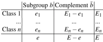
LetT be a training set of examples labelled bynclassesC1,...,Cn. We denote the total
number of examples in the training set byEand the number of examples belonging to classCibyEi. The number of examples inT covered by a subgroupbis denoted bye,
and the number of examples belonging toCi and covered bybis denoted byei. This
notation is summarised in Table 1; all evaluation measures considered in this paper are based on numbers in such a contingency table.
Aheuristicis defined as ann-dimensional functionRn→Rsuch thath(e1,...,en)
represents the quality of subgroupb, whereeiare as in Table 1. We will often
abbrevi-ate this toh(b)if no confusion can arise. We will use the terms heuristic and evaluation measure interchangeably in the rest of the paper. Following [4], we will use the follow-ing definition for comparfollow-ing the different heuristics.
Definition 1 (Compatibility and Antagonism [4] ).Two heuristic functions h1and h2
arecompatibleiff for all subgroups b1, b2: h1(b1)>h1(b2) ⇐⇒ h2(b1)>h2(b2). h1
and h2areantagonisticiff for all subgroups b1, b2: h1(b1)>h1(b2) ⇐⇒ h2(b1)<
h2(b2). h1and h2areequivalent(h1∼h2) if they are either compatible or antagonistic.
Table 1.Notational conventions for the frequencies in a multi-class contingency table tabulating examples covered or not covered by a given subgroupb
SubgroupbComplement ¯b
Class 1 e1 E1−e1 E1
... ... ... ...
Classn en En−en En
The intuition is that equivalent heuristics order the search space in the same way, even if they differ in numerical value. For instance,h(x)∼Enh(x), sinceEandnare constants for a given data set. However,h(x)∼EE−eh(x), sinceedepends on the subgroup.
CN2is a rule induction algorithm that can be applied to propositional data sets for inducing classification rules [5, 6]. A propositional data set can be thought of as a sin-gle database table with rows representing examples and columns representing features. CN2 consists of two main algorithms: the search algorithm that performs beam search1 in order to find a single rule and the covering algorithm that repeatedly executes the search for rules until all examples are covered. The search algorithm searches the rule space top-down, evaluating the quality of rules using precision (the relative frequency of positives among the examples covered). A rule takes the form of (head←body) where the body is a conjunction of body literals and the head is a single head literal indicating a class. A literal takes the form of (feature Op value) whereOpcan be one of the following three operators:>,<or=.
CN2 can apply a significance test to each rule being learned. If there is a regularity unlikely to have occurred by chance, then the rule is regarded as significant. Further-more, a minimum evaluation threshold can be used as a stopping criterion. When a rule achieves an evaluation value lower than this threshold, the search is pruned.
CN2 can induce rules in two forms: ordered list of rules and unordered set of rules. In the former, the search algorithm finds the best rule in the current set of training ex-amples. The rule predicts the class with the highest frequency among the examples it covers. All examples covered by the newly induced rule are removed before starting another search iteration. The rule search is repeated until all the examples are cov-ered. In the unordered setting, the main algorithm is iterated for each class in turn. For each induced rule, only covered examples belonging to the class being learned are removed.
CN2-SDis an extension of CN2 particularly geared towards subgroup discovery [1]. In subgroup discovery, one wants to find independent rules that may overlap. To that end, CN2-SD implements two major changes compared to CN2: replacing precision as a search heuristic withweighted relative accuracyor WRAcc (see Definition 2 in the next section), and the use of a weighted covering algorithm. While in the original cov-ering algorithm examples are removed once they are covered by a rule, in the weighted covering algorithm examples are never removed but their weight is decreased accord-ing to one of two schemes: additive or multiplicative. Letwt(x)denote the weight of
examplexafter being covered bytrules: in the additive method we havewt(x) = 1+1t
while in the multiplicative methodwt(x) =γt,0<γ<1.
The use of a weighting scheme, particularly the multiplicative weights, is related to the use of weights in AdaBoost [7], where an examplexat timet is re-weighted according towt(x) =wt−1(x)e−αtp; here,wt−1(x)is the current weight,αt =12ln1−εtεt
withεt<0.5 representing the error of the current hypothesis, and pis either 1 or−1
reflecting a correct or an incorrect prediction respectively. To obtain an update rule that is independent of the current hypothesis we set p=1 and εt =Emin, the size of the
1In beam search, thekmost promising candidate hypotheses are considered instead of all pos-sible candidate hypotheses for efficiency reasons.
minority class, which giveswt(x) =wt−1(x)
Emin
E−Emin. We therefore extended CN2-SD
with an option to set theγparameter for multiplicative weights to
Emin
E−Emin.
Another improvement in CN2-MSD, our version of CN2-SD for more than two classes, is the use of inequality with nominal values. Like CN2, CN2-SD uses only equality when constructing a new literal for a nominal feature, e.g. feature=val, whereas CN2-MSD also considers literals of the formfeature=val. Experiments sug-gest that the use of inequality slightly improves AUC as well as the accuracy.
3
Heuristics for Multi-class Subgroup Discovery
In this section we investigate possible heuristics for multi-class subgroup discovery. We start with considering multi-class versions of weighted relative accuracy in Section 3.1, followed by a consideration of other measures that are inherently multi-class in Sec-tion 3.2. In SecSec-tion 3.3 we consider the quesSec-tion whether a subgroup or its complement is the more interesting one.
3.1 Multi-class Versions of Weighted Relative Accuracy
Weighted relative accuracy was defined in a binary classification context [8]: here, we adapt it such that a given classCi is taken as positive and all other classes together as
the negative class. The idea is that the ruleaccuracy(which is actually the precision
ei
e) should be takenrelativeto the accuracy obtained by always guessingCi ( Ei
E), and
weightedby the rule’s coverage (Ee).
Definition 2 (Weighted Relative Accuracy [8]).The weighted relative accuracy of subgroup b for class Ciis defined as W RAcci(b) =Ee
ei e − Ei E =ei E− e E Ei E.
Previous research [9, 10, 11, 12] has investigated methods of multi-class classification. The methods usually decompose a multi-class problem into several binary problems either by considering all pairwise combinations of classes (one-vs-one) or considering each class against the union of the other classes (one-vs-rest). One model is trained for each binary problem and, according to the chosen method, the classification for an un-seen example is determined based on a competition of these binary models. It has been shown by [12, 10] that it is computationally expensive to perform the classification in such a manner because it requiresO(n)comparisons for each example to be classified. We are interested in obtaining a single final model, thus avoiding the computational costs of multiple binary comparisons during the classification phase.
The first idea might be to simply averageW RAcciover all classes. However, this will
fail due to the following simple result. Lemma 1. ∑ni=1W RAcci(b) =0. Proof. ∑ni=1W RAcci(b) =∑ni=1Ee ei e− Ei E = e E ∑n i=1eei −∑ n i=1EEi = e E[1−1] =0.
Definition 3 (Multi-class WRAcc).The (one-vs-rest) multi-class weighted relative ac-curacy is defined as MW RAcc(b) =1n∑ni=1|W RAcci(b)|.
Clearly, in a two-class setting,MW RAcc(b) =|W RAcci(b)|fori=1,2.
Rather than taking an unweighted average, we may want to take a weighted average using the class prior.
Definition 4 (Weighted Multi-class WRAcc).The (one-vs-rest) weighted multi-class weighted relative accuracy is defined as W MW RAcc(b) =∑ni=1Ei
E|W RAcci(b)|.
We can also define a one-vs-one version.
Definition 5 (One-vs-One Multi-class WRAcc).The one-vs-one multi-class weighted relative accuracy is defined as follows:
MW RAcc1vs1(b) = 1 n(n−1) n
∑
i=1 n∑
j=1;j=i |W RAcci j(b)| where W RAcci j(b) =Eei+ej i+Ej ei ei+ej − Ei Ei+Ej .Note that, whileW RAcci(b¯) =−W RAcci(b), for the multi-class versions defined here
we haveMW RAcc(b¯) =MW RAcc(b)and similar for the other measures.
We can further understand the similarities and differences between these heuristics by reducing them to simpler equivalent forms.
Theorem 1. MW RAcc∼∑ni=1|eiE−eEi|. Proof. MW RAcc=1n∑ni=1|Ee ei e − Ei E |= 1 nE2∑ n i=1|eiE−eEi| ∼∑ni=1|eiE−eEi|. Theorem 2. W MW RAcc∼∑ni=1Ei|eiE−eEi|. Proof. W MW RAcc=∑ni=1Ei E| e E ei e− Ei E |= 1 E3∑ n i=1Ei|eiE−eEi|∼∑ni=1Ei|eiE−eEi|. Theorem 3. MW RAcc1vs1∼∑n i=1∑nj=i+1 |eiEj−ejEi| (Ei+Ej)2 . Proof. Notice thatW RAcci j(b) =−W RAccji(b). Then,
MW RAcc1vs1= 1 n(n−1) n
∑
i=1 n∑
j=1;j=i |W RAcci j|= 2 n(n−1) n∑
i=1 n∑
j=i+1 |W RAcci j| ∼∑
n i=1 n∑
j=i+1 ei+ej Ei+Ej| ei ei+ej− Ei Ei+Ej| =∑
n i=1 n∑
j=i+1 |ei(Ei+Ej)−Ei(ei+ej)| (Ei+Ej)2 =∑
n i=1 n∑
j=i+1 |eiEj−ejEi| (Ei+Ej)2Thus, the key term in each of these heuristics is of the form|eiE−eEi|for one-vs-rest
measures and|eiEj−ejEi|for one-vs-one measures, possibly with weights depending
3.2 Other Multi-class Subgroup Evaluation Measures
In this section we consider other ways of evaluating the frequencies observed in an n-by-2 contingency table.
One possibility is to consider two random variables:Bis a binary variable indicating whether or not a random example is in the subgroup, andLis ann-ary variable indi-cating which class applies to that example. Given a contingency table, the marginal and joint entropies of these random variables are then as follows:
H(L) =− n
∑
i=1 Ei E log Ei E H(B) =−e Elog e E− E−e E log E−e E H(L,B) =− n∑
i=1 ei Elog ei E+ Ei−ei E log Ei−ei EWe can then define their mutual information in the usual way:MI(L,B) =H(L) + H(B)−H(L,B). Mutual information tells us how much knowledge about one variable would be increased by knowing the value of the other. The higher the mutual infor-mation, the more interesting the distribution of classes amongst the subgroup and its complement is.
Definition 6 (Mutual Information).The mutual information score of a subgroup b is defined as follows: MI(b) = n
∑
i=1 ei Elog ei E+ Ei−ei E log Ei−ei E −∑
n i=1 Ei Elog Ei E − e Elog e E− E−e E log E−e EAlternatively, we can use theChi-squaredtest to decide whetherLandBare statistically independent. Assuming that the data in Table 1 represents the observed frequencies, the expected values under the null hypothesis of independence of columns and rows can be calculated from the marginal frequencies. E.g., the expected value ofeiis eEEi. The
Chi-squared statistic is then the sum of the squared differences between observed and expected frequencies divided by the expected frequencies.
Definition 7 (Chi-Squared).The Chi-squared score of a subgroup b is defined as fol-lows: Chi2(b) = n
∑
i=1 [ei−EEie]2 Eie E +[(Ei−ei)−Ei(EE−e)]2 Ei(E−e) EFinally, we consider a decision tree splitting criterion based on the Gini index. Con-sider calculating the utility of a binary split in a multi-class context. A splitting criterion calculates the decrease in impurity when going from parent to children. The impurity of the children is calculated as the weighted average of their individual impurities, using the relative frequency of examples covered by the child as weight. The Gini index cal-culates the impurity of a node as1n∑ni=1pi(1−pi), wherepiis the relative frequency of
examples of classCi.
Definition 8 (Gini-split).The Gini-split score of a subgroup b is defined as follows: GS(b) = 1 n n
∑
i=1 Ei(E−Ei) E2 − 1 n n∑
i=1 e E ei(e−ei) e2 −1 n n∑
i=1 E−e E (Ei−ei)((E−Ei)−(e−ei)) (E−e)2 Theorem 4. Chi2=∑ni=1[eiE−eEi]2 eEi(E−e). Proof. Chi2=∑n i=1 [ei−eEiE ]2 eEi E +[(Ei−ei)−Ei(EE−e)]2 Ei(E−e) E = 1 E∑ n i=1[ eiE−eEi]2 eEi + [EiE−eiE−EiE+eEi]2 Ei(E−e) =1 E∑ n i=1[eiE−eEi]2 1 eEi+ 1 Ei(E−e) =1 E∑ n i=1[eiE−eEi]2EeEi(E2−e+e) i(E−e) =∑ n i=1[ eiE−eEi]2 eEi(E−e). Theorem 5. GS∼∑ni=1[eEi−eiE]2 e(E−e) . Proof. GS= 1n∑ni=1Ei(E−Ei) E2 − e E ei(e−ei) e2 − E−e E (Ei−ei)[(E−Ei)−(e−ei)] (E−e)2 = 1 nE∑ n i=1 Ei(E−Ei) E −ei(e−ei) e − (Ei−ei)[(E−Ei)−(e−ei)] E−e = 1 nE2∑ni=1 [eEi−eiE]2 e(E−e) ∼∑ n i=1 [eEi−eiE]2 e(E−e) .If thei-th term inChi2isxi, thei-th term inGSis equivalent toEixi. We can therefore
considerGSto be a class-weighted version ofChi2. This shows that, in general,Chi2∼ GS, thereby negatively answering an open question in [4]. They proved the equivalence in the binary case, and conjectured that this would extend to more than two classes. Theorem 6 (Equivalence of binary Chi-squared and Gini-split [4]). For n=2 classes, Chi2∼GS.
Proof. First of all,e1E−eE1=e1(E1+E2)−(e1+e2)E1=e1E2−e2E1. By symme-try,e2E−eE2=e2E1−e1E2. Therefore,[e1E−eE1]2= [e2E−eE2]2= [e1E2−e2E1]2. It follows thatChi2=
1 E1+ 1 E2 [e1E2−e2E1]2 e(E−e) = E E1E2 [e1E2−e2E1]2
e(E−e) . On the other hand,
GS=2E12
2[e1E2−e2E1]2
e(E−e) = E1E2
E3 Chi2.
It is interesting to note that our proof of Theorem 6 is much more succinct than the one given in [4]. It appears the multi-class notation is beneficial here.
Measures similar toChi2andGSwere used previously in the Explora system [2, 3]. Explora is an interactive knowledge discovery system that incorporates several search
strategies, refinement methods and evaluation functions. If we distinguish Kl¨osgen’s definitions by a subscriptKl, we can show the equivalence between ourChi2andGS measures and Kl¨osgen’s as follows:
GSKl(b) = e E E−e E n
∑
i=1 ei e− Ei E 2 = e E−e n∑
i=1 e2i e2+ Ei2 E2− 2eiEi eE = e E2(E−e) n∑
i=1 e2Ei2+ei2E2−2eieEi e2 = 1 E2 n∑
i=1 [eEi−eiE]2 e(E−e) = 1 nGS(b) Chi2Kl(b) = 1 E2 n∑
i=1 [eEi−eiE]2 e(E−e) Ei E = 1 E n∑
i=1 [eEi−eiE]2 eEi(E−e) = 1 EChi 2(b)Although our definitions ofChi2andGSare not equal to Kl¨osgen’s definitions they are indeed equivalent, henceChi2∼Chi2Kl andGS∼GSKl.
3.3 Sign of a Subgroup
In two-class subgroup discovery a subgroup correlates positively with one class if and only if its complement correlates negatively with the other class. This can eas-ily be established by, e.g., the sign ofW RAcci(b); we generally restrict attention to
the subgroup that has positive weighted relative accuracy for the designated positive class. For the multi-class case we propose a criterion for determining whether a sub-group or its complement is the more interesting one based on conditional entropy. We have H(L|B=b) =∑ni=1ei
elog ei
e, the entropy of the left column of the
contin-gency table; and similarly H(L|B=b¯) =∑in=1EEi−−eeilog Ei−ei
E−e. The sign of the
sub-group is then sign(H(L|B=b¯)−H(L|B=b)). If the amount of uncertainty remain-ing aboutLassumingB=b is smaller than when assumingB=b¯, then the sign of H(L|B=b¯)−H(L|B=b)is positive, favouringbover ¯b.
4
Empirical Evaluation
We performed extensive experiments to test the behaviour of the six subgroup evalua-tion measures defined in the previous secevalua-tion, as well as the usefulness of multi-class subgroup discovery for feature generation in a classification context. We used 20 UCI data sets [14], which are listed in Table 2. Numerical attributes with more than 100 dis-tinct values have been discretised. Our implementation of CN2-MSD is an adaptation of the CN2-SD implementation provided by the authors of [1], which was implemented in Java as part of the Weka data mining workbench [15]. Six different settings have been applied as follows:
– setting 0: unweighted covering;
– setting 1: multiplicative weights,γ=.25; – setting 2: multiplicative weights,γ=.5;
Table 2.UCI data sets used for the experiments. CMC stands for Contraceptive Method Choice while WPBC stands for Wisconsin Prognostic Breast Cancer.
Dataset Name #exs. # attrs. # cls. Dist.
1 Abalone 4176 9 3 1527, 1342 and 1307 2 Balance-scale 624 5 3 288, 288 and 48 3 Car 1727 7 4 1209, 384, 69 and 65 4 CMC 1472 10 3 628, 511 and 333 5 Contact-lenses 24 5 3 15, 5 and 4 6 Credit 589 16 2 383 and 306 7 Dermatology 365 35 6 112,72, 60, 52, 49 and 20 8 Glass 213 11 6 76, 69, 29, 17, 13 and 9 9 Haberman 305 4 2 224 and 81 10 Hayes-roth 131 5 3 51, 50 and 30 11 House-votes 434 17 2 267 and 167 12 Ionosphere 350 34 2 224 and 126 13 Iris 150 5 3 50, 50 and 50 14 Labor 57 17 2 37 and 20 15 Mushroom 8123 23 2 4208 and 3915 16 Pima-indians 767 9 2 500 and 267 17 Soybean 683 36 19 92, 2×91, 88, 2×44, 9×20, 16, 15, 14 and 8 18 Tic-Tac-Toe 957 10 2 625 and 332 19 WPBC 197 34 2 150 and 47 20 Zoo 100 18 7 40, 20, 13, 10, 8, 5 and 4
Table 3.Average number of subgroups found on 20 UCI data sets using different heuristics and settings
Setting MW RAcc1vs1MW RAcc W MW RAcc MI Chi2 GSaverage
0 5.70 6.25 5.95 6.90 6.80 7.15 6.46 1 9.20 10.05 9.50 14.55 13.55 14.25 11.85 2 11.50 12.15 12.30 20.30 20.65 20.70 16.27 3 16.65 16.40 17.00 26.20 27.90 28.05 22.03 4 14.50 15.30 15.65 30.10 31.00 31.10 22.94 5 10.40 9.60 9.40 15.30 15.55 17.00 12.88 Average 11.33 11.63 11.63 18.89 19.24 19.71
– setting 3: multiplicative weights,γ=.75; – setting 4: additive weights; and
– setting 5: multiplicative weights,γ=
Emin
E−Emin.
The significance and minimum evaluation threshold parameters were fixed to 0.95 and 0.01, respectively.
The first result concerns the number of subgroups found (as reported in Table 3). It is clear that the WRAcc-based methods find significantly fewer subgroups than the other three. Weighted covering clearly helps in finding more subgroups. Additive weights and multiplicative weights with largeγ (i.e., slow decay of the weights) result in the most subgroups. Settingγ=
Emin
−1 0 1 2 3 4 5 6 7 8 2 3 4 5 6 Setting Number Rank Accuracy MWRAcc 1vs1 MWRAcc WMWRAcc MI Chi−squared Gini−Split Decision Tree −1 0 1 2 3 4 5 6 7 8 2 3 4 5 6 Setting Number Rank AUC MWRAcc 1vs1 MWRAcc WMWRAcc MI Chi−squared Gini−Split Decision Tree
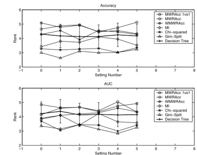
Fig. 1.Accuracies and AUCs of the multi-class subgroup discovery methods compared with the J48 control learner (bold line). For each setting, performances outside the vertical bar are signifi-cantly better (bottom) or worse (top) than the control.
In order to evaluate the quality and utility of the induced subgroups, we use them as features for a decision tree learner. We use the Weka implementation of C4.5 which is called J48, with default parameters. 10-fold cross-validated accuracy and AUC are recorded on each data set, for J48 run directly on the original data set (labelled J48 in our result tables) and J48 run using subgroups as features, where the subgroups are learned using CN2-MSD with one of the six evaluation heuristics (labelled with that heuristic in the table), and for each of the six settings.
For space reasons we only report averages over all 20 data sets in Tables 4 and 5 (all subsequent tables can be found in the Appendix). Average accuracies and AUCs have limited meaning because the values are not necessarily commensurate across data sets, and so we also report the average rank (1 is best, 7 is worst) of a method across all data sets. We use the Friedman test on these average ranks (p=0.10) with Bonferroni-Dunn post-hoc test to check significance against J48 as a control learner. The Friedman test records wins and losses in the form of ranks, but ignores the magnitude of these wins and losses, which is considered more appropriate when comparing multiple classifiers on multiple data sets; see [16] for more details. A graphical illustration of the post-hoc test results is given in Fig. 1. For each setting the corresponding critical difference diagram is shown vertically. So, for instance, in setting 4 bothMI andGS perform significantly better than J48, and in setting 5MW RAcc1vs1performs significantly worse than J48.
Tables 6-8 show the results for number of leaves, number of nodes in the tree and the model construction times. As can be seen, the average tree has roughly between 8 and 16 times fewer leaves when trained with subgroups as features, compared with standard
−1 0 1 2 3 4 5 6 7 8 2 3 4 5 6 7 8 Setting Number Rank Number of Leaves MWRAcc 1vs1 MWRAcc WMWRAcc MI Chi−squared Gini−Split Decision Tree −1 0 1 2 3 4 5 6 7 8 0 1 2 3 4 5 6 Setting Number Rank
Model Construction Time
MWRAcc 1vs1 MWRAcc WMWRAcc MI Chi−squared Gini−Split Decision Tree
Fig. 2.Number of leaves and model construction times of the multi-class subgroup discovery methods compared with the J48 control learner (bold line)
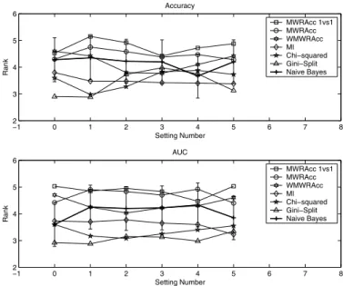
−1 0 1 2 3 4 5 6 7 8 2 3 4 5 6 Setting Number Rank Accuracy MWRAcc 1vs1 MWRAcc WMWRAcc MI Chi−squared Gini−Split Naive Bayes −1 0 1 2 3 4 5 6 7 8 2 3 4 5 6 Setting Number Rank AUC MWRAcc 1vs1 MWRAcc WMWRAcc MI Chi−squared Gini−Split Naive Bayes
Fig. 3.Accuracies and AUCs of the multi-class subgroup discovery methods compared with the naive Bayes control learner (bold line)
J48, and roughly between 6 and 12 times fewer nodes. This comes, of course, at the expense of considerable additional execution time. Fig. 2 shows this graphically (the ranks in Tables 6 and 7 are equal and therefore the two graphs for number of leaves and number of nodes are identical).
Finally, we report accuracy and AUC results using naive Bayes as the learner (Fig. 3). The results are similar as for J48, although differences between evaluation measures are less pronounced. Tables 9-11 show the average accuracies, AUCs and model construc-tion times of the multi-class subgroup discovery methods compared with naive Bayes as a control classifier.
Our conclusions from these experiments are that the multi-class subgroup evaluation measures considered in this paper can be divided into two groups. The WRAcc-based measures result on average in much fewer subgroups (although the model construction time is not significantly reduced). If the subgroups are used for prediction, the additional subgroups learned byMI and particularlyChi2andGSresult in additional predictive power compared to the base learner. A consistently good performer isGS in combi-nation with multiplicative weights,γ=0.25 (setting 1) or additive weights (setting 4). Given that setting 4 is an order of magnitude slower, we finally settle on setting 1 as our recommendation. This combination achieves significantly higher predictive power than the base learners, building trees that on average have 11 times fewer leaves.
5
Related Work
As discussed earlier, CN2-MSD is an upgrade of the CN2-SD rule learner [1] which learns two-class subgroups and was in turn based on the CN2 inductive rule learner [5, 6]. More details about CN2 and CN2-SD were given in Section 2. Our three multi-class Weighted Relative Accuracy versions are multi-multi-class adaptations of the two-multi-class Weighted Relative Accuracy that originated in [8] and was incorporated in CN2-SD.
Mutual information is used to measure dependencies between random variables. Mu-tual information is appropriate for assessing the information content of features in com-plex classification tasks. It has been used for feature selection [17, 18]. The difference between the usage of MI in [17, 18] and CN2-MSD is that CN2-MSD uses MI to eval-uate a combination of one or more features, rather than comparing single features. MI as used in [18] also differs from our approach in that it selects features that maximise the MI with respect to a single class but not all the classes. In addition, CN2-MSD only assesses the constructed feature and its complement while this is not the case in the other two approaches due to having different goals.
Chi-squared has been used widely as a statistical significance test in various con-texts including classification and rule learning. Chi-squared was found useful for fea-ture selection [13]. The original CN2-SD uses a Chi-squared significance test to filter a nominated subgroup in case it yields a value lower than a certain minimum value.2 CN2-MSD implements the Chi-squared as a heuristic function similarly to the Explora system [2].
Gini-split is well-known in decision tree learning as a splitting criterion based on the Gini index that evaluates the decrease in impurity when going from parent to
children. Gini-split is traditionally used in the divide and conquer (DAQ) paradigm where the learning algorithm divides the entire training set recursively according to a new selected literal. An example can not be covered by more than one rule or leaf in the final model. CN2-MSD, however, uses Gini-split in the separate and conquer (SAC) paradigm as it implements a sequential covering algorithm (and its weighted version). In SAC, single or multiple rules are learned iteratively and the examples covered by the learned rules are removed from the training set before proceeding to the next it-eration until no examples are left or a stopping criterion met. In covering algorithms, a subset of the training examples (or weighted training examples) is used to construct rules iteratively. An example could be covered by more than one rule or leaf in the final model. Induction systems that implement SAC are less conservative in their learning model than the ones that implement DAC due to their ability to explore a larger search space [19].
Explora is an interactive knowledge discovery system for databases [2, 3]. Explora was designed to support analysts in finding new knowledge about a domain. It can be used for predictive learning as well as descriptive learning. Explora is a complex system that incorporates various search strategies (exhaustive or heuristic), refinement methods and evaluation functions for binary and multi-class prediction. Explora can also work with relational data. It can be viewed as a generic pattern discovery system in relational data mining.
Another system related to CN2-MSD is called PRIM [20]. PRIM finds subregions of the instance space within which the value of the (continuous) output variable is con-siderably larger or smaller than its average value over the entire space. PRIM searches for these subregions by top-down specialisation followed by a bottom-up generalisation on the induced subgroups. Further criteria are needed to ensure capturing subgroups of reasonable size. One of the advantages of using WRAcc is that it captures the the gen-erality of the subgroupEe and its relative accuracyei
e− Ei
E in a single score. While CN2
uses a greedy refinement strategy on partial candidate hypotheses, PRIM examines all possible solutions which makes it unsuitable for large datasets.
The work of [4] provided us with the basis for the theoretical analysis of multi-class subgroup evaluation measures. Two-class Weighted Relative Accuracy, Chi-squared and Gini-split were discussed and analysed in [4] and their ROC isometrics visually and analytically compared. Unfortunately, a fulln-class ROC analysis requiresn(n−1)/2 dimensions, and so it is hard – if not impossible – to visualise multi-class evaluation measures through their ROC isometrics.
6
Conclusions
In this paper we upgraded existing approaches for two-class subgroup discovery to han-dle more than two classes. We defined six multi-class subgroup evaluation measures and investigated their properties theoretically and experimentally. While multi-class sub-group discovery is an interesting task in its own right, located between predictive and descriptive learning, we have also shown that – if the additional computational cost can be justified – the learned subgroups lead to additional predictive power. In effect, the decision trees learned branch on more complex multivariate conditions, and the naive Bayes classifier relaxes its assumptions of statistical independence.
In future work we plan to study whether subgroup discovery can be exploited in other predictive tasks, such as probability estimation and regression. We also aim to investigate multi-class subgroup discovery in a relational context. Furthermore, we will focus on reducing the computational overhead of subgroup discovery.
References
1. Lavraˇc, N., Kavˇsek, B., Flach, P., Todorovski, L.: Subgroup Discovery with CN2-SD. Journal of Machine Learning Research 5, 153–188 (2004)
2. Kl¨osgen, W.: Explora: A multipattern and multistrategy discovery assistant. In: Fayyad, U.M., Piatetsky-Shapiro, G., Smyth, P., Uthurusamy, R. (eds.) Advances in Knowledge Dis-covery and Data Mining, pp. 249–271. MIT Press, Cambridge (2004)
3. Kl¨osgen, W.: Subgroup discovery. In: Kl¨osgen, W., Zytkow, J.M. (eds.) Handbook of Data Mining and Knowledge Discovery, pp. 354–361. Oxford University Press, Oxford (2002) 4. F¨urnkranz, J., Flach, P.: ROC ’n’ rule learning: Towards a better understanding of covering
algorithms. Machine Learning 58, 39–77 (2005)
5. Clark, P., Niblett, T.: The CN2 Induction Algorithm. Machine Learning 3, 261–283 (1989) 6. Clark, P., Boswell, R.: Rule induction with CN2: Some recent improvements. In: Kodratoff,
Y. (ed.) EWSL 1991. LNCS (LNAI), vol. 482, pp. 151–163. Springer, Heidelberg (1991) 7. Schapire, R.E.: The boosting approach to machine learning: An overview. In: Nonlinear
Es-timation and Classification. Lecture Notes in Statistics. Springer, Heidelberg (2003) 8. Lavraˇc, N., Flach, P., Zupan, B.: Rule evaluation measures: A unifying view. In: Dˇzeroski,
S., Flach, P.A. (eds.) ILP 1999. LNCS (LNAI), vol. 1634, pp. 174–185. Springer, Heidelberg (1999)
9. Friedman, J.H.: Another approach to polychotomous classification. Technical report, Stan-ford University, Department of Statistics (1996)
10. Kijsirikul, B., Ussivakul, N., Meknavin, S.: Adaptive directed acyclic graphs for multiclass classification. In: Ishizuka, M., Sattar, A. (eds.) PRICAI 2002. LNCS (LNAI), vol. 2417, pp. 158–168. Springer, Heidelberg (2002)
11. Platt, J.C., Cristianini, N.: Large margin DAGs for multiclass classification. In: Advance in Neural Information Processing Systems, vol. 12. MIT Press, Cambridge (2000)
12. Hsu, C.W., Lin, C.J.: A comparison of methods for multiclass support vector machines. Neu-ral Networks 13, 415–425 (2002)
13. Jin, X., Xu, A., Bie, R., Guo, P.: Machine Learning Techniques and Chi-Square Feature Se-lection for Cancer Classification Using SAGE Gene Expression Profiles. In: Li, J., Yang, Q., Tan, A.-H. (eds.) BioDM 2006. LNCS (LNBI), vol. 3916, pp. 106–115. Springer, Heidelberg (2006)
14. Newman, D., Hettich, S., Blake, C., Merz, C.: UCI repository of machine learning databases (1998)
15. Witten, I.H., Frank, E.: Data Mining: Practical Machine Learning Tools and Techniques, 2nd edn. Morgan Kaufmann, San Francisco (2005)
16. Demˇsar, J.: Statistical comparisons of classifiers over multiple data sets. Journal of Machine Learning Research 7, 1–30 (2006)
17. Battiti, R.: Using mutual information for selecting features in supervised neural net learning. Transactions on Neural Networks 5(4) (1994)
18. Fleuret, F.: Fast binary feature selection with conditional mutual information. Journal of Machine Learning Research 5, 1531–1555 (2004)
19. Bostrom, H.: Covering vs. divide-and-conquer for top-down induction of logic programs. In: Proceedings of the Fourteenth International Joint Conference on Artificial Intelligence, pp. 1194–1200. Morgan Kaufmann, San Francisco (1995)
20. Friedman, J.H., Fisher, N.I.: Bump hunting in high-dimensional data. Statistics and Comput-ing 9, 123–143 (1999)
Appendix: Detailed Experimental Results
Table 4.Accuracies (ranks in brackets) of a decision tree learner using subgroups as features, averaged over 20 UCI data sets
Setting MW RAcc1vs1 MW RAcc W MW RAcc MI Chi2 GS J48
0 75.11 (5.08) 76.95 (4.65) 77.90 (4.28) 77.40 (3.42) 78.24 (3.27) 79.87 (3.00) 81.21 (4.30) 1 76.90 (4.78) 78.40 (4.88) 79.95 (4.55) 78.14 (3.80) 80.47 (3.20) 81.85 (2.63) 81.21 (4.17) 2 76.75 (4.92) 78.80 (4.95) 80.52 (3.92) 80.19 (3.73) 81.37 (3.25) 81.34 (3.10) 81.21 (4.13) 3 77.85 (4.47) 78.95 (4.45) 80.31 (4.55) 80.03 (4.10) 81.08 (3.30) 81.64 (3.00) 81.21 (4.13) 4 76.63 (4.75) 78.83 (4.55) 80.34 (4.45) 80.33 (3.95) 81.33 (3.02) 81.48 (3.02) 81.21 (4.25) 5 75.28 (5.13) 77.70 (4.33) 79.05 (4.28) 78.94 (3.52) 79.42 (3.35) 79.96 (3.23) 81.21 (4.17)
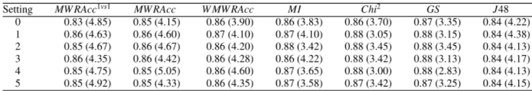
Table 5.AUCs (ranks in brackets) of a decision tree learner using subgroups as features, averaged over 20 UCI data sets
Setting MW RAcc1vs1 MW RAcc W MW RAcc MI Chi2 GS J48
0 0.83 (4.85) 0.85 (4.15) 0.86 (3.90) 0.86 (3.83) 0.86 (3.70) 0.87 (3.35) 0.84 (4.22) 1 0.86 (4.63) 0.86 (4.60) 0.87 (4.10) 0.87 (4.10) 0.88 (3.05) 0.88 (3.15) 0.84 (4.38) 2 0.85 (4.67) 0.86 (4.67) 0.86 (4.20) 0.88 (3.42) 0.88 (3.45) 0.88 (3.45) 0.84 (4.13) 3 0.86 (4.35) 0.86 (4.42) 0.86 (4.28) 0.86 (4.22) 0.88 (3.42) 0.88 (3.13) 0.84 (4.17) 4 0.85 (4.75) 0.85 (5.05) 0.86 (4.60) 0.87 (3.65) 0.88 (3.00) 0.88 (2.83) 0.84 (4.13) 5 0.85 (4.92) 0.85 (4.33) 0.86 (4.35) 0.87 (3.58) 0.87 (3.42) 0.87 (3.25) 0.84 (4.15)
Table 6.Numbers of leaves (ranks in brackets) of a decision tree learner using subgroups as features, averaged over 20 UCI data sets
Setting MW RAcc1vs1 MW RAcc W MW RAcc MI Chi2 GS J48
0 7.55 (2.95) 8.30 (3.48) 8.05 (3.20) 8.25 (4.10) 9.45 (3.67) 9.40 (4.05) 122.05 (6.55) 1 8.65 (3.30) 10.00 (3.30) 9.15 (3.52) 9.85 (3.52) 9.25 (3.50) 11.00 (4.28) 122.05 (6.58) 2 8.45 (2.77) 9.50 (2.90) 10.45 (3.52) 9.20 (3.80) 11.30 (4.38) 11.35 (4.08) 122.05 (6.55) 3 11.80 (3.25) 11.00 (2.90) 13.05 (3.77) 11.70 (3.63) 11.95 (3.85) 13.00 (4.15) 122.05 (6.45) 4 8.80 (2.80) 10.90 (2.77) 12.40 (3.50) 13.90 (4.25) 12.00 (4.05) 12.75 (4.17) 122.05 (6.45) 5 10.45 (3.23) 8.90 (3.13) 7.70 (3.10) 11.60 (3.88) 11.60 (3.98) 14.55 (4.17) 122.05 (6.53)
Table 7.Tree sizes (ranks in brackets) of a decision tree learner using subgroups as features, averaged over 20 UCI data sets
Setting MW RAcc1vs1 MW RAcc W MW RAcc MI Chi2 GS J48
0 14.10 (2.95) 15.60 (3.48) 15.10 (3.20) 15.50 (4.10) 17.90 (3.67) 17.80 (4.05) 162.05 (6.55) 1 16.30 (3.30) 19.00 (3.30) 17.30 (3.52) 18.70 (3.52) 17.50 (3.50) 21.00 (4.28) 162.05 (6.58) 2 15.90 (2.77) 18.00 (2.90) 19.90 (3.52) 17.40 (3.80) 21.60 (4.38) 21.70 (4.08) 162.05 (6.55) 3 22.60 (3.25) 21.00 (2.90) 25.10 (3.77) 22.40 (3.63) 22.90 (3.85) 25.00 (4.15) 162.05 (6.45) 4 16.60 (2.80) 20.80 (2.77) 23.80 (3.50) 26.80 (4.25) 23.00 (4.05) 24.50 (4.17) 162.05 (6.45) 5 19.90 (3.23) 16.80 (3.13) 14.40 (3.10) 22.20 (3.88) 22.20 (4.03) 28.10 (4.22) 162.05 (6.42)
Table 8.Model construction times (ranks in brackets) of a decision tree learner using subgroups as features, averaged over 20 UCI data sets
Setting MW RAcc1vs1 MW RAcc W MW RAcc MI Chi2 GS J48
0 5.93 (3.83) 6.40 (4.88) 6.61 (4.65) 6.33 (3.77) 6.67 (4.60) 6.46 (5.28) 0.23 (1.00) 1 21.73 (3.92) 22.61 (4.13) 20.22 (3.30) 27.80 (4.63) 32.40 (5.30) 33.57 (5.72) 0.23 (1.00) 2 43.00 (3.83) 40.36 (3.50) 42.80 (3.65) 51.36 (5.28) 45.68 (5.28) 41.39 (5.47) 0.23 (1.00) 3 90.32 (3.33) 83.43 (3.25) 89.39 (3.83) 106.30 (5.00) 105.01 (5.97) 104.17 (5.63) 0.23 (1.00) 4 232.41 (3.67) 238.21 (3.08) 232.53 (3.92) 147.71 (5.47) 158.16 (5.42) 167.92 (5.42) 0.23 (1.00) 5 100.99 (4.17) 111.30 (4.15) 105.34 (3.58) 99.43 (5.15) 67.40 (4.85) 70.05 (5.10) 0.23 (1.00)
Table 9.Accuracies (ranks in brackets) of a naive Bayes learner using subgroups as features, averaged over 20 UCI data sets
Setting MW RAcc1vs1 MW RAcc W MW RAcc MI Chi2 GS NB
0 73.76 (4.53) 75.08 (4.30) 75.42 (4.60) 76.31 (3.80) 76.78 (3.60) 78.82 (2.90) 79.86 (4.28) 1 75.74 (5.15) 77.49 (4.75) 79.32 (4.42) 78.39 (3.48) 80.04 (2.98) 81.44 (2.88) 79.86 (4.35) 2 75.39 (4.92) 77.73 (4.58) 79.79 (3.80) 79.37 (3.48) 80.51 (3.27) 79.83 (3.73) 79.86 (4.22) 3 75.63 (4.42) 77.20 (4.38) 79.58 (3.77) 78.85 (3.42) 79.22 (3.83) 79.39 (3.98) 79.86 (4.20) 4 74.98 (4.72) 77.02 (4.47) 79.18 (4.10) 78.24 (3.40) 77.66 (3.88) 78.37 (3.75) 79.86 (3.67) 5 74.99 (4.88) 77.14 (4.28) 78.25 (4.42) 78.47 (3.38) 78.03 (3.73) 79.27 (3.13) 79.86 (4.20)
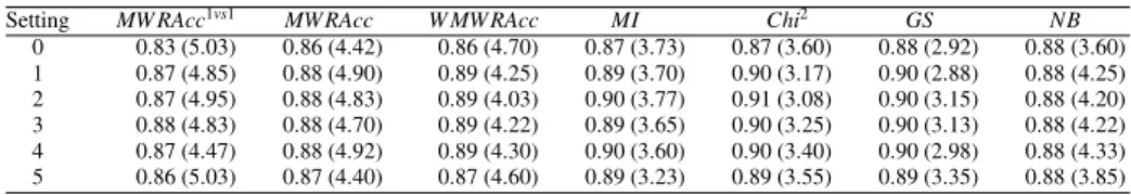
Table 10.AUCs (ranks in brackets) of a naive Bayes learner using subgroups as features, averaged over 20 UCI data sets
Setting MW RAcc1vs1 MW RAcc W MW RAcc MI Chi2 GS NB
0 0.83 (5.03) 0.86 (4.42) 0.86 (4.70) 0.87 (3.73) 0.87 (3.60) 0.88 (2.92) 0.88 (3.60) 1 0.87 (4.85) 0.88 (4.90) 0.89 (4.25) 0.89 (3.70) 0.90 (3.17) 0.90 (2.88) 0.88 (4.25) 2 0.87 (4.95) 0.88 (4.83) 0.89 (4.03) 0.90 (3.77) 0.91 (3.08) 0.90 (3.15) 0.88 (4.20) 3 0.88 (4.83) 0.88 (4.70) 0.89 (4.22) 0.89 (3.65) 0.90 (3.25) 0.90 (3.13) 0.88 (4.22) 4 0.87 (4.47) 0.88 (4.92) 0.89 (4.30) 0.90 (3.60) 0.90 (3.40) 0.90 (2.98) 0.88 (4.33) 5 0.86 (5.03) 0.87 (4.40) 0.87 (4.60) 0.89 (3.23) 0.89 (3.55) 0.89 (3.35) 0.88 (3.85)
Table 11.Model construction times (ranks in brackets) of a naive Bayes learner using subgroups as features, averaged over 20 UCI data sets
Setting MW RAcc1vs1 MW RAcc W MW RAcc MI Chi2 GS NB
0 6.13 (3.92) 6.38 (4.53) 6.53 (3.95) 6.82 (4.45) 6.97 (5.13) 6.27 (5.03) 0.05 (1.00) 1 21.34 (3.85) 21.17 (4.03) 21.62 (4.03) 27.14 (4.33) 30.06 (5.25) 32.01 (5.53) 0.05 (1.00) 2 40.80 (4.08) 41.21 (3.50) 42.54 (3.50) 50.33 (5.25) 44.47 (5.17) 42.89 (5.50) 0.05 (1.00) 3 86.51 (3.42) 84.38 (3.63) 89.06 (3.35) 107.75 (5.00) 104.10 (5.70) 113.92 (5.90) 0.05 (1.00) 4 218.62 (3.35) 228.58 (3.60) 242.22 (4.13) 135.36 (5.22) 163.41 (5.28) 160.14 (5.42) 0.05 (1.00) 5 96.66 (3.90) 97.59 (3.92) 99.19 (4.22) 94.14 (4.92) 69.53 (5.13) 70.79 (4.90) 0.05 (1.00)