MPG Prediction Using Artificial Neural Network

(1)

Vol. 4 Issue 11, November - 2020, Pages: 7-16

MPG Prediction Using Artificial Neural Network

Yara Ibrahim Al Barsh, Maram Khaled Duhair, Hassan Jassim Ismail, Bassem S. Abu-Nasser, Samy S. Abu-Naser Department of Information Technology,

Faculty of Engineering & Information Technology, Al-Azhar University - Gaza, Palestine

Abstract: During the course of this research, imposing the training of an artificial neural network to predicate the MPG rate for present thru forthcoming automobiles in the foremost relatively accurate evaluation for the approximated number which foresight the actual number to help through later design and manufacturing of later automobile, by training the ANN to accustom to the relationship between the skewing of each later stated attributes, the set of mathematical combination of the sequences that could be excavate the Miles Per Gallon(MPG) by the system and using both the Gradient Descent Algorithm and the Normalized Square Error Technique explicitly lure the Final Parameter Norm and Scaling layer and Bounded Layering rules implicitly. And so on the system should be able to produce immune approximations `and calculations to make better of results of What the Actual output estimation.

Keywords: ANN, artificial neural network, automobile, fuel efficiency, predict fuel consumption 1.INTRODUCTION

While the thermal efficiency (mechanical output to chemical energy in fuel) of petroleum engines has increased since the beginning of the automotive era to a current maximum of 36.4% this is not the only factor in fuel economy. The design of automobile as a whole and usage pattern affects the fuel economy. Published fuel economy is subject to variation between jurisdictions due to variations in testing protocols.

One of the first studies to determine fuel economy in the United States was the Mobil Economy Run, which was an event that took place every year from 1936 (except during World War II) to 1968. It was designed to provide real fuel efficiency numbers during a coast to coast test on real roads and with regular traffic and weather conditions. The Mobil Oil Corporation sponsored it and the United States Auto Club (USAC) sanctioned and operated the run. In more recent studies, the average fuel economy for new passenger car in the United States rose from 17 mpg in 1978 to more than 22 mpg in 1982.2The average fuel economy in 2008 for new cars, light trucks and SUVs in the United States was 26.4 mpgUS (8.9 L/100 km).3 2008 model year cars classified as "midsize" by the US EPA ranged from 11 to 46 mpgUS(21 to 5 L/100 km)4 However, due to environmental concerns caused by CO2 emissions, new EU regulations are being introduced to reduce the average emissions of cars sold beginning in 2012, to 130 g/km of CO2, equivalent to 4.5 L/100 km (52 mpgUS, 63 mpgimp) for a diesel-fueled car, and 5.0 L/100 km (47 mpgUS, 56 mpgimp) for a gasoline (petrol)-fueled car[5].

The average consumption across the fleet is not immediately affected by the new vehicle fuel economy: for example, Australia's car fleet average in 2004 was 11.5 L/100 km (20.5 mpgUS) [6], compared with the average new car consumption in the same year of 9.3 L/100 km (25.3 mpgUS)[7].

Problem Statement

In this project we will train an Artificial Neural Network (ANN) to give better estimates for MPG rates all over the automobile industry. The learning method involved is feed-forward learning. Such calculation would help to reduce the efforts needed to design and analyze automobile fuel consumption with such limited factors “attributes (cylinders, displacement factor, horsepower, weight, acceleration, model year and origins of manufacturing).

2.ARTIFICIALNEURALNETWORKS

The historical prospect

Warren McCulloch and Walter Pitts [8] (1943) created a computational model for neural networks based on mathematics and algorithms called threshold logic. This model paved the way for neural network research to split into two approaches. One approach focused on biological processes in the brain while the other focused on the application of neural networks to artificial intelligence. This work led to work on nerve networks and their link to finite automata[9].

Artificial Neural Network;

(2)

Perceptron-type neural networks consist of artificial neurons or nodes, which are information processing units arranged in layers and interconnected by synaptic weights (connections). Neurons can filter and transmit information in a supervised fashion in order to build a predictive model that classifies data stored in memory.

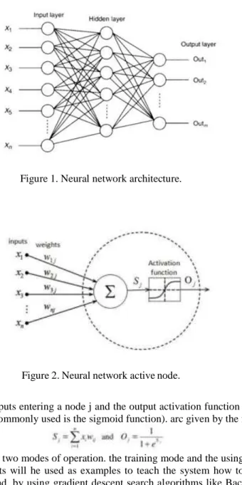
Typical ANN model is a three-layered network of interconnected nodes: the input layer, the hidden layer, and the output layer. The nodes between input and output layers can form one or more hidden layers. Every neuron in one layer has a link to every other neuron in the next layer, but neurons belonging to the same layer have no connections between them (Figure 1). The input layer receives information from the outside world, the hidden layer performs the information processing and the output layer produces the class label or predicts continuous values. The values from the input layer entering a hidden node are multiplied by weights, a set of predetermined numbers, and the products are then added to produce a single number. This number is passed as an argument to a nonlinear mathematical function, the activation function, which returns a number between 0 and 1 [11].

Figure 1. Neural network architecture.

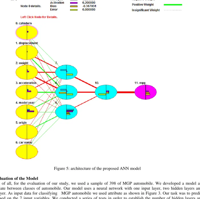
Figure 2. Neural network active node.

In Fig.2, the net sum of the weighted inputs entering a node j and the output activation function that converts n neuron's weighted input to its output activation (the most commonly used is the sigmoid function). arc given by the following equations respectively.

The neuron. and therefore the ANN. has two modes of operation. the training mode and the using mode. During the training phase, a data set with actual inputs and outputs will he used as examples to teach the system how to predict outputs. This supervised learning begins with random weights and, by using gradient descent search algorithms like Backpropagntion, adjusts the weights to be applied to the task at hand. The difference between target output values and obtained values is used in the error function to drive learning [12]. The error function depends on the weights. which need to be modified in order to minimize the error. For a given training set {(x1,t1), (x2,t2),···.(xk.tk)} consisting of k ordered pairs of n inputs andm dimensional vectors(n-inputs,

(3)

m-Vol. 4 Issue 11, November - 2020, Pages: 7-16

outputs), which are called the input and output patterns, the error for the output of each neuron can he defined by the equation: E1 = 1/2(oj – tj)2. while the error function of the network that must be minimized is given by:

while Oj is the output produced when the input pattern Xj from the training set enters the network. and t1 is the target value [11]. During the training mode, each weight is changed adding to its previous value the quantity

where is a constant that gives the learning rule. The higher the learning rate, the faster the convergent will be. but the searching path may trapped around the optimal solution and convergence become impossible. Once a set of good weights have been found, the neural network model can take another dataset with unknown output values and predict automatic the corresponding outputs.

3.1 MPG Definition

The fuel economy of an automobile is the relationship between the distance traveled and the amount of fuel consumed by the vehicle. Consumption can be expressed in terms of volume of fuel to travel a distance, or the distance travelled per unit volume of fuel consumed. Since fuel consumption of vehicles is a significant factor in air pollution, and since importation of motor fuel can be a large part of a nation's foreign trade, many countries impose requirements for fuel economy. Different methods are used to approximate the actual performance of the vehicle. The energy in fuel is required to overcome various losses (wind resistance, tire drag, and others) encountered while propelling the vehicle, and in providing power to vehicle systems such as ignition or air conditioning. Various strategies can be employed to reduce losses at each of the conversions between the chemical energy in the fuel and the kinetic energy of the vehicle. Driver behavior can affect fuel economy; maneuvers such as sudden acceleration and heavy braking waste energy.

Fuel economy is the relationship between the distance traveled and fuel consumed.

Fuel economy can be expressed in two ways: Units of fuel per fixed distance

Generally expressed as liters per 100 kilometers (L/100 km), used in most European countries, China, South Africa, Australia and New Zealand. British and Canadian law allow for the use of either liters per 100 kilometers or miles per imperial gallon.15 Recently, the window sticker on new US cars has started displaying the vehicle's fuel consumption in US gallons per 100 miles, in addition to the traditional MPG number[12].

The Corporate Average Fuel Economy (CAFE) regulations in the United States, first enacted by Congress in 1975,17 are federal regulations intended to improve the average fuel economy of cars and light trucks (trucks, vans and sport utility vehicles) sold in the US in the wake of the 1973 Arab Oil Embargo. Historically, it is the sales-weighted average fuel economy of a manufacturer's fleet of current model year passenger cars or light trucks, manufactured for sale in the United States. Under Truck CAFE standards 2008–2011 this changes to a "footprint" model where larger trucks are allowed to consume more fuel. The standards were limited to vehicles under a certain weight, but those weight classes were expanded in 20S’.

(4)

The JustNN tool was used to develop the ANN model. The structure of the neural network was set as feed-forward, in which the output layer connects only to the previous layer. ANN training used 67% of the 398 cases and 33% of cases were selected for the validation set.

All cases were randomly selected by the JustNN tool. The parameters considered the input layer for the neural network training can be seen in the following adjacent figures, combined with other parameters describing the combinations of the tic-tac-toe game regression. A total of eight input parameters were used in the development of the ANN model (see Appendix). Several configurations of ANN were tested in other to find the best performing combination of number of hidden layers and nodes per layer. In all configurations, Eq. was used as activation function to smooth the output signal of each node:

where x is the sum of the weighted input of each previous node plus the bias of the node itself. ANN results were evaluated based on the coefficient of determination of all strategies possible to the game mind, the mean bias error -

The role of uncertainty in the ANN predictions was investigated with the support of additional ANNs. In these additional ANN, the uncertain parameters were not included as input variable. The accuracy of these ANNs was then compared to the accuracy of the original ANN (which includes all eight input parameters).

Once the role of uncertainty was clarified, the sensitivity of the ANN to different input parameters was investigated. For this purpose, ANN was used to calculate 1 additional variation for each one of the 398 original simulation cases. In these variations, only one parameter was change at a time using the 8 discreet input values. This procedure allowed the calculation of individual changes in the single output due to individual changes in each one of the inputs. Uncertainty was not taken into account in the sensitivity analysis.

5.1 Data Set

The data set contains the information for creating the predictive model[13]. It comprises a data matrix in which columns represent variables and rows represent instances. Variables in a data set can be of three types: The inputs will be the independent variables; the targets will be the dependent variables; the unused variables will neither be used as inputs nor as targets. Additionally, instances can be: Training instances, which are used to construct the model; selection instances, which are used for selecting the optimal order; testing instances, which are used to validate the functioning of the model; unused instances, which are not used at all.

5.2 Variables table

The following table depicts the names, units, descriptions and uses of all the variables in the data set. The numbers of inputs, targets and unused variables here are 7, 1, and 0, respectively.

Table1: attributes of the dataset

# Attribute name Scope Type of

attribute

1 mpg continuous Input

2 cylinders multi-valued discrete Input

(5)

4 horsepower continuous Input

5 weight continuous Input

6 acceleration continuous Input

7 model year multi-valued discrete Input

8 origin multi-valued discrete Input

9 car name string (unique for each instance) Output

5.3 Neural network parameters

The following figure shows the parameters of the proposed neural network model. The total number of parameters is 20, like learning rate and momentum.

Figure3: Shows the Control parameter of ANN model

5.4 Scaling Data

The size of the un-scaling layer is 1, the number of outputs. The un-scaling method for this layer is the minimum and maximum. The following table shows the values which are used for scaling the inputs, which include the minimum, maximum, mean and standard deviation. The data after scaling is shown in Figure 4.

(6)

Figure4: Scaled dataset

5.5 Neural network graph

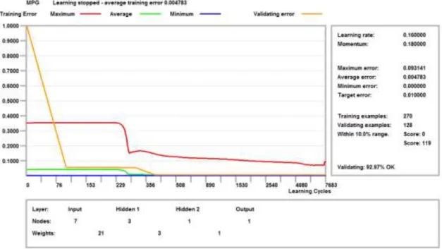
A graphical representation of the network architecture is depicted next. It contains a scaling layer, a neural network. The yellow circles represent scaling neurons, the green circles the principal components, the blue circles perceptron neurons, the red circles un-scaling neurons, and the purple circles bounding neurons. The number of inputs is 7, the number of principal components is 7, and the number of outputs and bounding neurons are 1. The complexity, represented by the numbers of hidden neurons, is 3:1 (as seen in Figure 5).

(7)

Figure 5: architecture of the proposed ANN model

5.6 Evaluation of the Model

First of all, for the evaluation of our study, we used a sample of 398 of MGP automobile. We developed a model able to differentiate between classes of automobile. Our model uses a neural network with one input layer, two hidden layers and one output layer. As input data for classifying MGP automobile we used attribute as shown in Figure 3. Our task was to predict the result based on the 7 input variables. We conducted a series of tests in order to establish the number of hidden layers and the number of neurons in each hidden layer. Our tests give us that the best results are obtained with two hidden layer. We used a sample of (398 records): 270 training samples and 128 validating samples. The network structure was found on a trial and error basis (as seen in Figure 5). We started with a small network and gradually increased its size. Finally, we found that the best results are obtained for a network with the following structure: 7I-2H-1O, i.e. 7 input neurons, 2 hidden layers with (3x1) neurons, and an output layer with 1 neuron. For this study we used Just Neural Network (JNN)[57]. We trained the network for 7683 epochs (as shown in Figure 6) on a regular computer with 4 GB of RAM memory under the Windows 10 operating system. We got an accuracy of 92.97%. Figure 3 shows Parameters of the proposed ANN model. Figure 7 shows the factors, their importance and relative importance that affect the MGP automobile artificial Neural Model using Just NN environment. Figure 8 outlines the detail of the proposed ANN model.

(8)

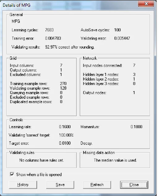
Figure 6: Training and validation of the proposed ANN model

(9)

Figure 8: Details of the proposed ANN model

3. CONCLUSION

Data pre-processing helps in producing cleaning data which can be used in building a more accurate architecture. Table provided in the testing section shows the comparison between the results obtained for auto mpg data set using various algorithms on same data. Algorithms used (Normalized Squared Error + Gradient Descent).

In This paper, we used the classification power of a neural network to classify auto mpg. Our network achieved an accuracy of 92.977%. We used the JustNN environment for building the network that was a feed forward Multi-Layer Perceptron with one input layer, two hidden layer and one output layer. The average predictability rate was 92.97% for classification of MGP automobile.

References

1. Koichiro Muta, Makoto Yamazaki, Junji Tokieda, Development of New-Generation Hybrid System THS II - Drastic Improvement of Power Performance and Fuel Economy 2004-01-0064

2. Paul R. Portney; Ian W.H. Parry; Howard K. Gruenspecht; Winston Harrington (2003). "The Economics of Fuel Economy Standards" . Resources For The Future. Retrieved 4 January 2020.

(10)

5. Badia, M.; Qian, J.P.; Fan, B.L. Artificial neural networks and thermal image for temperature prediction in apples. Food Bioprocess Technol. 2012, 9, 1089–1099. [CrossRef]

6. Nunes, M.C.N.; Nicometo, M.; Emond, J.P.; Badia-Melis, R.; Uysal, I. Improvement in fresh fruit and vegetable logistics quality: Berry logistics field studies. Philos. Trans. R. Soc. A Math. Phys. Eng. Sci. 2014, 372, 20130307.

7. Raab, V.; Petersen, B.; Kreyenschmidt, J. Temperature monitoring in meat supply chains. Br. Food J. 2011, 113, 1267– 1289.

8. Katic, K.; Li, R.L.; Verharrt, J.; Zeiler, W. Neural network based predictive control of personalized heating systems. Energy Build. 2018, 174, 199–213. [CrossRef]

9. Li, X.M.; Zhao, T.Y.; Zhang, J.L.; Chen, T.T. Predication control for indoor temperature time-delay using Elman neural network in variable air volume system. Energy Build. 2017, 154, 545–552.

10. Mercier, S.; Uysal, I. Neural network models for predicting perishable food temperatures along the supply chain. Biosyst. Eng. 2018, 171, 91–100.

11. Thenozhi, S.; Yu, W. Stability analysis of active vibration control of building structures using PD/PID control. Eng. Struct. 2014, 81, 208–218.

12. Guerrero, J.; Torres, J.; Creuze, V.; Chemori, A.; Campos, E. Saturation based nonlinear PID control for underwater vehicles: Design, stability analysis and experiments. Mechatronics 2019, 61, 96–105.

13. UCI Machine Learning repository (https://archive.ics.uci.edu/ml/datasets.html) 14. EasyNN Tool