Implicit Fixed-point Proximity Framework for Optimization Problems and Its Applications

SURFACE

SURFACE

Dissertations - ALL SURFACE

June 2018

Implicit Fixed-point Proximity Framework for Optimization

Implicit Fixed-point Proximity Framework for Optimization

Problems and Its Applications

Problems and Its Applications

Syracuse University

Follow this and additional works at: https://surface.syr.edu/etd

Part of the Physical Sciences and Mathematics Commons

Recommended Citation Recommended Citation

Liu, Xiaoxia, "Implicit Fixed-point Proximity Framework for Optimization Problems and Its Applications" (2018). Dissertations - ALL. 897.

https://surface.syr.edu/etd/897

This Dissertation is brought to you for free and open access by the SURFACE at SURFACE. It has been accepted for inclusion in Dissertations - ALL by an authorized administrator of SURFACE. For more information, please contact

A variety of optimization problems especially in the field of image processing are not differentiable in nature. The non-differentiability of the objective functions together with the large dimension of the underlying images makes minimizing the objective function the-oretically challenging and numerically difficult. The fixed-point proximity framework that we will systematically study in this dissertation provides a direct and unified methodology for finding solutions to those optimization problems. The framework approaches the models arising from applications straightforwardly by using various fixed point techniques as well as convex analysis tools such as the subdifferential and proximity operator.

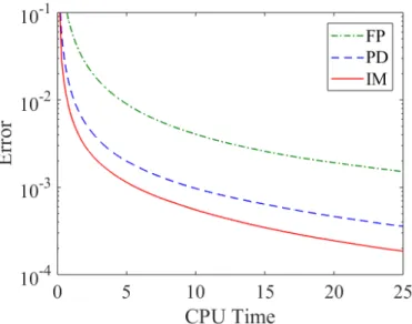
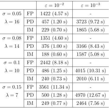
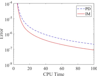
With the notion of proximity operator, we can convert those optimization problems into finding fixed points of nonlinear operators. Under the fixed-point proximity framework, these fixed point problems are often solved through iterative schemes in which each iteration can be computed in an explicit form. We further explore this fixed point formulation, and develop implicit iterative schemes for finding fixed points of nonlinear operators associated with the underlying problems, with the goal of relaxing restrictions in the development of solving the fixed point equations. Theoretical analysis is provided for the convergence of implicit algorithms proposed under the framework. The numerical experiments on image reconstruction models demonstrate that the proposed implicit fixed-point proximity algo-rithms work well in comparison with existing explicit fixed-point proximity algoalgo-rithms in terms of the consumed computational time and accuracy of the solutions.

Optimization Problems and Its Applications

By

Xiaoxia Liu

B.S., Sun Yat-sen University, 2012 M.S., Syracuse University, 2016

Dissertation

Submitted in partial fulfillment of the requirements for the degree of Doctor of Philosophy in Mathematics

Syracuse University June 2018

First and foremost, I would like to express my deepest gratitude to both of my advisors, Professor Yuesheng Xu and Professor Lixin Shen, for their patient guidance, constant inspi-ration and generous support in the past six years. They have not only taught me knowledge in convex analysis and fixed point theory, skills in problem posing and problem solving, and techniques in scientific writing and presenting, but they have also enlightened me to fulfill my academic dreams with their expertise, rigorous thinking and enthusiasm. All their guidance will be beneficial to my future career and life. In addition, I greatly appreciate the time that they spent in discussing with me, providing me insightful feedback and correcting my mistakes. I would never have been able to finish my dissertation without their help.

I also sincerely appreciate my committee members, Professors Dan Coman, Eugene Polet-sky, Minghao Rostami and Bei Yu for taking time to review my dissertation and providing helpful feedback. I am grateful to the faculty members and staff at Syracuse University, especially Professors Uday Banerjee, Pinyuen Chen, Graham Leuschke, Adam Lutoborski, and Grace Wang for their inspiring courses and help.

I am thankful to all my colleagues and friends for making my life in Syracuse enjoyable. I would like to thank, Feishe Chen, Lei Chen, Stephen Farnham, Rachel Gettinger, James Heffers, Qian Huang, Lei Jin, Muzhi Jin, Hyesu Kim, Si Li, Yuzhen Liu, Wenting Long, Xuefei Ma, Hani Sulieman, Erin Tripp, Agya Wagya and Yihe Yu. Special thanks to my lovely friends, Casey Necheles, Chen Liang, Alice Lim, Mkrtich Ohanyan, Mingyue Wang, Jinxia Xie and Jing Zhou for their warm encouragement and support not only through the

Finally, I would like to express my sincerest appreciation to my parents Sumei Xie and Chaoxin Liu, and my siblings for their selfless love and faith. Special thanks to my beloved partner Dingqiang Ma for his continued understanding, patience and support over these years.

Acknowledgements iv

1 Introduction 1

1.1 Problem Statement . . . 1

1.2 Literature Review . . . 5

1.3 Motivations . . . 7

1.4 Contributions of This Dissertation . . . 8

1.5 Organization of This Dissertation . . . 9

2 Implicit Fixed-point Proximity Framework 10 2.1 Notations and Preliminaries . . . 11

2.1.1 Preliminaries in convex analysis . . . 12

2.1.2 Preliminaries in fixed point theory . . . 15

2.2 Fixed Point Characterization . . . 17

2.3 Fixed-point Proximity Framework . . . 20

2.4 Existing Fixed-point Proximity Algorithms . . . 24

2.5 Implicit Fixed-point Proximity Framework . . . 29

2.5.1 Preliminaries on contractive mappings . . . 30

2.5.2 Implicit fixed-point proximity algorithm . . . 31

2.5.3 Property 1: LM is an M-operator . . . 33

2.5.4 Property 2: LM can be evaluated efficiently . . . 35

2.5.6 Possible block structures of M for implicit algorithms . . . 39

2.5.7 Convergence analysis . . . 40

3 Examples of Implicit Fixed-point Proximity Algorithms 48 3.1 Example 1 . . . 49

3.1.1 Fixed point characterization . . . 50

3.1.2 Existing fixed-point proximity algorithms . . . 52

3.1.3 Implicit fixed-point proximity algorithm . . . 53

3.1.4 Convergence analysis . . . 55

3.2 Example 2 . . . 59

3.2.1 Fixed point characterization . . . 59

3.2.2 Existing fixed-point proximity algorithms . . . 61

3.2.3 Implicit fixed-point proximity algorithms . . . 62

3.2.4 Convergence analysis . . . 66

3.3 Other Examples . . . 76

3.3.1 Fixed point characterization . . . 76

3.3.2 Implicit fixed-point proximity algorithms . . . 78

4 Applications in Image Processing and Numerical Experiments 80 4.1 Applications in Image Processing . . . 80

4.1.1 Image reconstruction models . . . 81

4.1.2 Total variation regularization . . . 81

4.2 Application of Example 1: Total Variation Based Denoising Models . . . 82

4.2.1 Parameter settings . . . 83

4.2.2 ROF model . . . 84

4.2.3 L1-TV model . . . 87

4.2.4 Sensitivity of parameter settings . . . 90

4.3.1 Parameter settings . . . 95 4.3.2 L2-TV model . . . 95 4.3.3 L1-TV model . . . 97

5 Conclusion and Future Work 100

Introduction

1.1

Problem Statement

In this dissertation, the optimization problem of our interest is to minimize a sum of convex functions composed with linear operators

min x∈Rn N X i=1 fi(Aix), (P0)

where _Rn denotes the usual n-dimensional Euclidean space, Ai is an mi ×n matrix, and

fi :Rmi →(−∞,+∞] is proper, lower semi-continuous and convex, i= 1,2, . . . , N.

The optimization problem (P0) is motivated by many applications including image pro-cessing and machine learning. Some examples of its applications are shown as follows.

(i) Applications in image processing

In image processing, an observed image z degraded by blurring or/and noise can be modeled as z = Kx +η, where x represents the unknown image to be recovered,

K represents the measurement process, and η represents the additive noise. Image reconstruction models for approximatingxare usually formulated as a sum of one data fidelity term and at least one regularization term. The data fidelity term measures,

adapting to the noise type of η, the similarity between the observed image z and the desired image x. The regularization term is included to explore the prior structures of the underlying image. The most popular choice of the regularization term in image processing is the total variation [10, 74] defined as

k · kT V =ψ◦D,

where D is a first order difference matrix, and ψ is the `1 norm k · k1 or a certain

linear combination of the `2 norm k · k2 in R2 [32, 51]. Besides the total variation

regularization, there are other regularization terms such as the framelet regulariza-tion term [7, 8, 47], which is defined as the `1 norm of the framelet coefficients of the

underlying image under a framelet transformation.

In each of the following image reconstruction models, the first term is corresponding to the data fidelity term, the second term (and the third term if any) is corresponding to the regularization term, and λ >0 andµ > 0 are model parameters.

• Rudin-Osher-Fatemi (ROF) Model [74]: The model is designed to restore an

image contaminated by Gaussian noise, and can be written as problem (P0) with

f1 = λ₂k · −zk22, A1 =I, f2 =ψ, A2 =D, i.e., min x λ 2kx−zk 2 2+kxkT V. (M1)

• L1-TV Denoising Model [12, 65]: The model is designed to restore an image

contaminated by impulsive noise (or called pepper-and-salt noise), and can be written as problem (P0) withf1 =λk · −zk1, A1 =I, f2 =ψ, A2 =D, i.e.,

min

• L2-TV Image Restoration Model [2, 13, 67]: The model is designed to restore a blurry image contaminated by Gaussian noise, and can be written as problem (P0) with f1 = λ₂k · −zk22, A1 =K, f2 =ψ, A2 =D, i.e., min x λ 2kKx−zk 2 2+kxkT V. (M3)

• L1-TV Image Restoration Model[22,41]: The model is designed to restore a blurry image contaminated by impulsive noise, and can be written as problem (P0) with

f1 =λk · −zk1, A1 =K, f2 =ψ, A2 =D, i.e.,

min

x λkKx−zk1+kxkT V. (M4)

• Framelet Based Image Reconstruction Models [6, 34, 54]: The models are similar to the total variation based image reconstruction models mentioned above, except that the total variation regularization term is replaced by the framelet regular-ization term [7, 8], which can be written as a composition of the `1 norm k · k1

and a linear operator Dwhere Drepresents a tight frame system generated from framelets [47].

• MR Image Reconstruction Model [46, 58, 59, 84]: The model is designed to recon-struct an MR image x that is sparse in the wavelet domain. Let Φ be a given sampling matrix, b be observed measurements, and W be a wavelet transform. The model can be written as problem (P0) with f1 = 1₂k · −bk22, A1 = Φ, f2 =

ψ, A2 =D, f3 =k · k1, A3 =W, i.e., min x λ 2kΦx−bk 2 2+µkxkT V +kW xk1. (M5)

(ii) Applications in machine learning

function possibly along with a regularization term. The loss function describes the expected cost, and the most frequently used regularization term is the`1 regularization

term that enforces sparsity on the desired solution in order to avoid over-fitting [78].

• The `1-regularized Linear Least Squares Problem: This problem is known as

Basis Pursuit [9, 21, 29] in compressive sensing and Least Absolute Shrinkage and Selection Operator (LASSO) [78] in machine learning and statistics. Ba-sis pursuit is designed to recover a sparse signal x from compressed measure-ments. Let Φ be a given sampling matrix, b be observed measurements, and

λ be a model parameter. The model can be written as problem (P0) with

f1 = λ₂k · −bk22, A1 = Φ, f2 =k · k1, A2 =I, i.e., min x λ 2kΦx−bk 2 2+kxk1. (M6)

• The `1-regularized Classification Model [28, 76, 81]: The model is designed for

classifying data by using a linear classifier in machine learning. Supposew∈ _Rn

is the sparse coefficients of the linear classifier to be computed, b∈_R is the bias of the linear classifier,λ >0 is a model parameter, (xi, yi)∈Rn×Rare the given

data points, and li : R → R are loss functions, i = 1,2, . . . , N. The model can

be written as problem (P0) with f1(w) = λPN_i=1li(yi(w>xi +b)), A1 = In, f2 = k · k1, A2 =In, i.e., min w λ N X i=1 li(yi(w>xi+b)) +kwk1.

There are several classification models that can be written in this form with different choice of the loss function li. For example, support vector machine

(SVM) [28,81] uses the hinge loss function and logistic regression optimization [76] uses the logistic loss function.

cost in a network with N agents. Suppose x is the solution to be computed, and

fi is the cost function of thei-th agent,i= 1,2, . . . , N. The model can be written

as problem (P0) with Ai =I, i.e.,

min x N X i=1 fi(x).

All the optimization problems mentioned above can be solved by the algorithms developed under the implicit fixed-point proximity framework that we will propose in this dissertation. Depending on the number of convex functions and the number of composite linear operators, the applicable algorithms are different. We will illustrate in detail the fixed-point proximity framework with an emphasis on implicit algorithms in Chapter 2.

1.2

Literature Review

The fixed-point proximity framework for composite optimization problems has been ex-tensively studied in recent years due to its ease of applicability. The framework relies on the notion of proximity operator, which was introduced early in [62, 73] and widely adopted to applications arising from image processing (see, e.g., [4, 5, 27]). Under the fixed-point prox-imity framework, the solutions of the optimization problem are characterized as fixed points of a mapping defined in terms of proximity operator, thereby allowing for the development of efficient numerical methods via various powerful fixed point iterations.

The first algorithm, developed from the perspective of both proximity operator and fixed point theory, was the fixed point problem algorithm based on proximity operator (FP2O) [60] designed to solve the ROF model (M1) for image denoising. Accordingly, this fixed-piont proximity approach has been extended to handle the L1-TV model (M2) for image denoising [17, 50, 61], the basis pursuit model (M6) for compressive sensing [15], the TV-regularized MAP ECT reconstruction model for ECT image reconstruction [49], the exp-model for removing multiplicative noise [56, 57], and other exp-models [53].

Various algorithms have been proposed since then by employing the fixed-point proximity framework along with other techniques in convex analysis and numerical analysis. For exam-ple, the multi-step fixed-point proximity algorithm [51, 52] introduced the multi-step scheme into the framework; the primal–dual fixed point algorithm based on proximity operator (PDFP2O) [18–20] combined the framework with the primal dual formulation [11,69,82]; the fixed-point proximity Gauss-Seidel algorithm (FPGS) [16] utilized the Gauss-Seidel method and a parameters relaxation technique in addition to the framework.

The fixed-point proximity framework has been demonstrated in the literature to be a powerful tool for composite optimization problems [51]. On one hand, the framework pro-vides a general platform to explore new algorithms for different optimization problems. On the other hand, the framework offers new insights on existing algorithms and puts forward new improvements.

Many existing algorithms can be identified as a fixed-point proximity algorithm and be reinterpreted under the framework, even though they are developed from different per-spectives. We classify these algorithms roughly into two categories. The first category of algorithms are developed from the Fenchel-Rockafellar duality theory [25, 72] and have the primal dual formulation [69, 82]. The primal dual method formulates a primal problem and a dual problem, and then updates the primal variable and dual variable alternatively. For example, first order primal dual algorithm (PD) [11, 69, 82], primal-dual hybrid gradient algorithm (PDHG) [33, 87], and contraction-type primal dual algorithm [43] are considered as fixed-point proximity algorithms in the first category. The second category of algorithms are developed from the augmented Lagrangian technique [37, 44, 70, 71]. The augmented La-grangian method minimizes the augmented LaLa-grangian function of the equality-constrained optimization problem, and then updates the Lagrange multipliers. For example, augmented Lagrangian method (ALM) [35–37, 44, 70, 71], alternating direction method of multipliers (ADMM) [3, 31, 36], and alternating minimization algorithm (AMA) [80] are considered as fixed-point proximity algorithms in the second category. Some algorithms based on splitting

techniques are shown to be closely related to the algorithms in the second category, including Douglas-Rachford splitting algorithm (DRSA) [26, 31], alternating split Bregman iteration (ASBI) [39], and Bregman operator splitting algorithm (BOS) [86].

1.3

Motivations

Among the algorithms for solving composite optimization problems, various algorithms can be reformulated as fixed-point proximity algorithms and further analyzed under the fixed-point proximity framework. Under this framework, the optimization problems are converted into fixed point problems in relation to proximity operators, and then be solved through iterative schemes. The existing fixed-point proximity algorithms all have anexplicit

iterative scheme so that the algorithms can be computed efficiently. However, we observe that there are some restrictions of those algorithms due to the explicitness. We are motivated to develop fixed-point proximity algorithms with a fully implicit scheme, because of the following restrictions of existing explicit fixed-point proximity algorithms.

First, the convergence assumptions of explicit fixed-point proximity algorithms may be relatively strict. For example, the primal dual algorithm (PD) has a relatively restricted selection range for the parameters of the proximity operators, which significantly influences the performance of the algorithm. That is due to the limitations of its underlying algorithm structure which is formed to maintain the explicit expression of the algorithm.

Second, the explicit fixed-point proximity algorithms may only be applicable to limited types of composite optimization problems. For example, the fixed point problem algorithm based on proximity operator (FP2O) and the alternating split Bregman iteration (ASBI) are designed to solve problems with quadratic functions. Additional numerical methods are employed to achieve the explicitness of those algorithms. But those numerical methods require additional assumptions not only on the parameters of the proximity operators but also on the objective function, which restricts the applicable range of the algorithms.

Therefore, we aim to study fixed-point proximity algorithms with a fully implicit scheme, because the implicit schemes allow more flexibility while building the structures of the al-gorithms, and have a potential to yield an algorithm that outperforms existing explicit algorithms.

1.4

Contributions of This Dissertation

In this dissertation, we establish an implicit fixed-point proximity framework that serves as a guideline for developing implicit iterative algorithms applied to composite optimization problems. We also propose several implicit algorithms under the framework with algorithm structures that are not observed in existing fixed-point proximity algorithms.

The two main contributions of this dissertation are summarized as follows.

• The first one is that we enrich the existing fixed-point proximity framework by an-alyzing fixed-point proximity algorithms with a fully implicit scheme. The existing framework is designed for developing algorithms with an explicit expression and is not applicable for developing algorithms with a fully implicit expression. Our proposed framework employs fixed point techniques, including contractive mappings, to address the issues that may occur while developing implicit algorithms. Theoretical results are provided to guarantee the convergence of implicit algorithms.

• The second one is that we propose two algorithm structures and develop several implicit fixed-point proximity algorithms for different composite optimization problems. We are not aware of any existing fixed-point proximity algorithms that possessed the pro-posed algorithm structures. And numerical experiments demonstrate that the implicit algorithms with the proposed algorithm structures outperform the existing fixed-point proximity algorithms in terms of computational time.

1.5

Organization of This Dissertation

This dissertation is organized in the following manner. In Chapter 2, we present the implicit fixed-point proximity framework. We start from fixed-point proximity equations that characterize the solutions of a composite optimization problem, and then build implicit algorithms via contractive mappings with comprehensive theoretical convergence results. In Chapter 3, we propose several implicit algorithms for different optimization problems under the implicit fixed-point proximity framework. For each implicit algorithm, we conduct a convergence analysis with theoretical results. In Chapter 4, we test the proposed implicit proximity algorithms on several image reconstruction models and demonstrate the practi-cal performance of the proposed implicit algorithms over other existing explicit fixed-point proximity algorithms. Finally, some conclusions and future work are presented in Chapter 5.

Implicit Fixed-point Proximity

Framework

In this chapter, we first review the existing fixed-point proximity framework for devel-oping explicit algorithms applied to composite optimization problems, and then propose a framework for developing fixed-point proximity algorithms with fully implicit schemes.

In order to formulate the fixed-point proximity framework in a general setting, we consider the optimization problem in the following general form

min

x∈Rn

f(Ax), (P1)

where A is an m×n matrix, and f : _Rm → (−∞,+∞] is proper, lower semi-continuous, and convex. By defining

A=          A1 A2 .. . AN          , y=          y1 y2 .. . yN          , and f(y) =PN

i=1fi(yi), problem (P0) can be written as problem (P1).

The rest of this chapter is organized in the following manner. In Section 2.1, we present 10

notations and recall some preliminary results in convex analysis and fixed point theory. Before illustrating the proposed implicit fixed-point proximity framework for problem (P1), we formulate in Section 2.2 fixed-point proximity equations that characterize the solutions of problem (P1), and then present a summary of the existing fixed-point proximity framework in Section 2.3 and a review of one class of existing fixed-point proximity algorithms in Section 2.4. Lastly, we present our main result in Section 2.5. We establish the implicit fixed-point proximity framework, which serves as a guideline for developing implicit algorithms.

2.1

Notations and Preliminaries

Let us introduce some notations and recall some preliminary results in convex analysis and fixed point theory.

For given x, y ∈ _Rd_{, hx, yi :=} Pd

i=1hxi, yii is the standard inner product and kxk2 := p

hx, xi is the standard `2 norm. Let Sd+ (resp. Sd) denote the set of symmetric positive

definite (resp. semi-definite) matrices of sized×dand letIddenote the identity matrix of size

d×d. For given x, y ∈ _Rd _{and a given H ∈}

Sd+, hx, yiH :=hx, Hyi is the H-weighted inner

product andkxkH := p

hx, xiH is the H-weighted`2 norm. IfH is the identity matrix, then

the H-weighted inner product reduces to the standard inner product, and the H-weighted

`2 norm reduces to the standard `2 norm.

Let f : _Rd _{→ (−∞,+∞]. The domain of f is a set in}

Rd defined as dom f := {x ∈ Rd : f(x) < +∞}. The function f is proper if dom f 6= ∅. The function f is lower

semi-continuous at a∈_Rd_{, iff(a)≤lim}

x→af(x). The functionf is convex if f(λx+ (1−λ)y)≤

λf(x) + (1−λ)f(y), for all x, y ∈ dom f, and all λ ∈ (0,1). The class of proper, lower semi-continuous, and convex functions from _Rd to (−∞,+∞] is denoted as Γ0(Rd).

2.1.1

Preliminaries in convex analysis

Let us present some preliminaries in convex analysis, which will be used in this disserta-tion.

First, we recall the definitions of several important concepts in convex analysis, including the subdifferential, conjugate, and proximity operator of a convex function.

For f ∈Γ0(Rd), the subdifferential of f at x∈Rd is a set in Rd defined as

∂f(x) :=y∈_Rd:f(u)≥f(x) +hy, u−xi for∀u∈_Rd . (2.1)

The elements of ∂f(x) are called the subgradients of f at x. Furthermore, ∂f(x) is a nonempty compact set for all x ∈dom f. In particular, if f is differentiable, then∂f(x) =

{∇f(x)}.

The conjugate of f is a mapping from _Rd to (−∞,+∞] defined as

f∗(y) := sup

x∈Rd

{hx, yi −f(x)}.

Iff ∈Γ0(Rd), then the conjugatef∗ ∈Γ0(Rd) and∂f∗(y) is a nonempty compact set for

ally ∈dom f∗. The subdifferentials of f and f∗ have the following relationship

y ∈∂f(x) if and only if x∈∂f∗(y). (2.2)

The proximity operator of f with respect toH ∈_Sd

+ is a mapping from Rd toRddefined

as prox_f,H(u) := argmin x∈_Rd f(x) + 1 2kx−uk 2 H . In particular, if H = 1

αId, α > 0, then proxf,H(u) reduces to the proximity operator with

parameter α with respect to the standard `2 norm, denoted as proxαf(u).

The proximity operator offwith respect toH ∈_Sd

off. The equationx= prox_f,H(u) holds if and only ifxis the unique solution of the following implicit problem        x=u−H−1_y y ∈∂f(x). (2.3)

The result above can be reinterpreted as follows by redefining the variableyin (2.3) asH−1_y,

Hy ∈∂f(x) if and only if x= prox_f,H(x+y). (2.4)

The relationship between the proximity operators of f and its conjugate f∗ is given by Moreau’s identity x= prox_f∗_,H(x) +H−1prox_f,H−1(Hx). (2.5) If f : _Rd → (−∞,+∞] can be written as f(x) = PN i=1fi(xi), where fi : Rdi → (−∞,+∞], xi ∈Rdi,i= 1, . . . , N, d=PNi=1di and x=          x1 x2 .. . xN          ,

then f is a block separable sum of fi’s, i = 1,2, . . . , N. The ith block of the proximity

operator of f is evaluated by the proximity operator of the ith separable part, that is,

prox_f(x)

i = proxfi(xi),

for i= 1,2, . . . , N.

Second, we present two examples for which we can explicitly compute their subdifferen-tials, conjugates and proximity operators.

Example 1: (Quadratic Function) We have ∂(1₂k · k2 2)(x) = {x}, 1 2k · k 2 2 ∗ = 1₂k · k2 2, and proxα 2k·k 2 2(x) = 1 α+1x.

Example 2: (The `2 Norm) Let ¯B(x, r) :={y∈Rd:kx−yk2 ≤r}denote a closed ball

center at x∈_Rd _{with radiusr >0. Then}

∂(k · k2)(x) =        n x kxk2 o , if x6= 0; ¯ B(0,1), if x= 0, (k · k2)∗(x) =ι_B¯_(0,1)(x) =        0, if x∈B¯(0,1); +∞, otherwise,

where ι_B¯_(0,1) is the indicator function of ¯B(0,1), and

prox_αk·k2(x) = max(kxk2 −α,0)

x

kxk2

.

Third, we start with some definitions and then present two important theorems for finding minimizers of a composite optimization problem.

The affine hull of a set S ⊆_Rd _{is a set in}

Rd defined as aff (S) := ( _k X i=1 αixi ∈Rd:k >0, xi ∈S, αi ∈R, k X i=1 αi = 1 ) .

The relative interior of a setS⊆_Rd_{is a set in}

Rdof all interior points ofS relative to aff (S)

defined as

ri (S) :={x∈S :∃ >0, B(x, )∩aff (S)⊆S},

where B(x, ) := {y ∈ _Rd _{: kx−yk}

2 < } is an open ball centered at x ∈ Rd with radius

>0.

which will be utilized to characterize the solutions of problem (P1).

The chain rule for the subdifferential of a convex functionf :_Rm _{→(−∞,+∞] composed}

with a linear operator A ∈ _Rm×n _{is stated as follows: If f ∈ Γ}

0(Rm) and Range (A)∩

ri (domf)6=∅, then

∂(f ◦A)(x) = A>∂f(Ax),

for all x∈_Rn_.

Fermat’s rule characterizes the global minimizers of a proper functionf :_Rd_{→(−∞,+∞]}

in terms of the subdifferential of f as follows

argminf =x∈_Rd _{: 0∈∂f(x) .}

2.1.2

Preliminaries in fixed point theory

Let us recall some definitions and helpful theorems in fixed point theory for develop-ing iterative algorithms, includdevelop-ing Krasnosel’skiˇı–Mann algorithm that will be used in this dissertation.

Definition 2.1 The set of fixed points of an operator T :_Rd_→

Rd is defined as

FixT :={x∈_Rd:x=T x}.

Definition 2.2 An operator T :_Rd_→

Rd is

(i) firmly nonexpansive with respect to H∈_Sd

+ if for all x, y ∈Rd

kT x−T yk2

(ii) nonexpansive with respect toH ∈_Sd

+ if for all x, y ∈Rd

kT x−T ykH ≤ kx−ykH;

(iii) α-averaged with respect to H ∈ _Sd

+, where α ∈ (0,1), if there exists a nonexpansive

operator R:_Rd→_Rd _{with respect to H ∈}

Sd+ such that T = (1−α)Id +αR.

Lemma 2.3 [25] Let f ∈ Γ0(Rd) and H ∈Sd+. Then proxf,H is firmly nonexpansive with

respect to H. If H = _α1Id, where α >0, then proxf,H = proxαf is firmly nonexpansive with

respect to the standard `2 norm.

Lemma 2.4 [25] LetT :_Rd_→

Rd and H ∈Sd+. Then

(i) T is firmly nonexpansive with respect to H if and only if for all x, y ∈_Rd

kT x−T yk2 H ≤ kx−yk 2 H − k(Id−T)x−(Id−T)yk 2 H;

(ii) T is α-averaged with respect to H, α∈(0,1), if and only if for allx, y ∈_Rd

kT x−T yk2 H ≤ kx−yk2H − 1−α α k(Id−T)x−(Id−T)yk 2 H;

(iii) T is firmly nonexpansive with respect to H if and only if T is 1₂-averaged with respect toH.

It is clear that a firmly nonexpansive operator is 1₂-averaged, and anα-averaged operator is nonexpansive. The nonexpansiveness of an operator T is sufficient to develop an iterative algorithm which generates a sequence converging to a point in Fix T, as demonstrated in the following theorem on Krasnosel’skiˇı–Mann algorithm.

Theorem 2.5 (Krasnosel’skiˇı–Mann Algorithm) Let T :_Rd_→

Rd be a nonexpansive

operator with respect to H ∈_Sd

+. Suppose that Fix T 6=∅. Let {λk} be a sequence in [0,1]

such that P

kλk(1−λk) = +∞. Then, for any initial vector x0 ∈ Rd, the sequence {xk}

generated by

xk+1 =xk+λk T xk−xk

converges to a point in Fix T.

Proof. The result follows from Theorem 5.14 in [25].

2.2

Fixed Point Characterization

With the preliminaries on convex analysis and fixed point theory in Section 2.1, we are ready to characterize the solutions of the optimization problem (P1) as the solutions of a system of fixed point equations in terms of proximity operators.

According to Fermat’s rule, a vector x∈ _Rn _{is a solution of problem (P1) if and only if}

the following inclusion relation holds

0∈∂(f◦A)(x). (2.6)

By applying equation (2.4) to the inclusion relation (2.6), the solution x of problem (P1) can be characterized as a fixed point of the proximity operator off ◦A with respect to any

P ∈_Sn

+, that is,

x= prox_f◦A,P(x). (2.7) However, it is rare to have an explicit expression of the proximity operator prox_f◦A,P for the optimization problems arising from image processing. Hence, it becomes necessary to exploit the composition nature of problem (P1) and to take advantage of the function f if

its proximity operator has a closed formula or is easy to evaluate.

Next, we apply the subdifferential chain rule to the composite functionf◦A, and obtain that the subdifferential of f ◦A evaluated at a point x is A>∂f(Ax). Then it follows from equations (2.3) that the fixed point equation (2.7) is equivalent to the following system

       x=x−P−1A>y y∈∂f(Ax). (2.8)

Note that the second equation in equations (2.8) can be converted into a fixed point equation in terms of the proximity operator of f∗ by using equation (2.2) and (2.4). Furthermore, the solutions of problem (P1) can be characterized as the solutions of a system of fixed point equations presented in the following proposition.

Proposition 2.6 Suppose that the set of solutions of problem (P1) is nonempty. If a vector x∈_Rn _{is a solution of problem (P1), then, for any P ∈}

Sn+ and Q∈Sm+, there exists

a vector y∈_Rm _{such that the following system of equations holds}        x=x−P−1_A>_y y= prox_f∗_,Q(y+Q−1Ax). (2.9)

Conversely, if there exist P ∈_Sn

+ and Q∈Sm+,x∈Rn, and y∈Rm satisfying the system of

equations (2.9), thenx is a solution of problem (P1).

Proof. It follows from Fermat’s rule and the subdifferential chain rule that x ∈ _Rn _{is a}

solution of problem (P1) if and only if there exists y ∈ _Rm _{such that y ∈ ∂f(Ax) and}

A>y= 0.

Suppose x ∈ _Rn _{is a solution of problem (P1). Let P ∈}

Sn+ and Q ∈ Sm+. It follows

from equation (2.2) thatQ(Q−1Ax)∈∂f∗(y). Thus, we deduce from equation (2.4) that the system of equations (2.9) holds.

Conversely, suppose that there exist P ∈_Sn

+ and Q∈Sm+, x∈Rn, andy∈Rm satisfying

the system of equations (2.9). Then A>y = 0. Also, it follows from equation (2.2) and equation (2.4) that y∈∂f(Ax). Thus,x is a solution of problem (P1).

Proposition 2.6 demonstrates that solving problem (P1) is equivalent to solving the sys-tem of fixed point equations (2.9). In fact, the syssys-tem of equations (2.9) is not the unique system of fixed point equations that can characterize the solutions. Other variants of equa-tions (2.9) can also be used to characterize the soluequa-tions as long as the soluequa-tions of fixed point equations (2.9) remain unchanged.

We present two variants of the fixed point equations (2.9). The first variant is gener-ated by substituting one of the fixed point equations into the other equations. The second variant is generated by applying Moreau’s identity (2.5) to rewrite the proximity operator if additional information on the objective function is provided.

Example 1: The first equation in equations (2.9) is a fixed point equation with respect to x, so we can replace the variable x in the second equation by the first equation with a parameter ˜P−1 _{different from P}−1_{. The new system of fixed point equations is shown as}

follows        x=x−P−1_A>_y y = prox_f∗_,Q(y+Q−1A(x−P˜−1A>y)). (2.10)

Example 2: Suppose that A = In. It follows from the first equation in equations (2.9)

that the variable y = 0 and thaty can be eliminated from the system. Then the first fixed point equation ofxcan be rewritten in terms of the proximity operator off instead off∗, by substituting the second equation into the variableyin the first equation, choosing P =Q−1, and then applying the Moreau’s identity (2.5). The new system of fixed point equations is shown as follows

All the fixed point equations mentioned above, including equations (2.9), (2.10) and (2.11), can be written as the following unified and compact fixed point equation

w= prox_F,R(Ew), (2.12)

where w∈_Rd_{, F :}

Rd →(−∞,+∞],R ∈Sd+ and E ∈Rd ×d_.

Equations (2.9) can be written as the unified fixed point equation (2.12) withF :_Rn+m _→

(−∞,+∞] defined by F(w) = f∗(y),R = diag (P, Q)∈_Sn+m + , w=    x y   ∈R n+m _{and E =}    In −P−1A> Q−1_{A I} m   ∈R (n+m)×(n+m)_.

Equations (2.10) can be written as equation (2.12) with the samew,F, andRas equations (2.9), but with a different matrix E defined as follows

E =    In −P−1A> Q−1_{A I} m−Q−1AP˜−1A>   ∈R (n+m)×(n+m)_{. (2.13)}

Equations (2.11) can be written as equation (2.12) with w = x ∈ _Rn_{, F :}

Rn →

(−∞,+∞] defined by F(x) = f(x), R=Q−1 _∈

Sn+ and E =In.

The unified fixed point equation (2.12) plays a fundamental role in the fixed-point prox-imity framework. It can represent a variety of fixed point equations that characterize the solutions of problem (P1), and allows us to formulate the fixed-point proximity framework in a general setting.

2.3

Fixed-point Proximity Framework

In this section, we present a general framework for developing algorithms to solve problem (P1). The framework is established based on the unified fixed point equation (2.12) in terms

of proximity operators, so we call this framework a fixed-point proximity framework. We start with equation (2.12) and then reformulate this equation to another equivalent fixed point equation, in order to develop convergent iterative algorithms.

The unified fixed point equation (2.12), which characterizes the solutions of problem (P1), is a fixed point equation of the composite operator prox_F,R ◦E. The proximity operator prox_F,R is always firmly nonexpansive with respect to R. However, kEk2 in most of the

scenarios is strictly great than 1 (see, e.g., [16, 51]). The composite operator prox_F,R ◦E

may not be nonexpansive, and the simple iterative algorithm wk+1 _{= prox}

F,R(Ewk) may not

converge. Thus, the operator prox_F,R ◦E has to be reformulated into another operator in order to generate a convergent algorithm.

In the fixed-point proximity framework, we split up the matrix E in equation (2.12) into two matrices M and E−M and then study the following implicit iterative algorithm

wk+1 = prox_F,R(M wk+1+ (E−M)wk), (2.14)

where M is a matrix to be determined later.

In order to have a better understanding of the implicit iterative algorithm (2.14), we introduce a new operatorLM induced from the implicit iterative scheme (2.14).

Definition 2.7 Let M be ad×d matrix. If for any vector u∈_Rd _{the following equation}

v = prox_F,R(M v+ (E−M)u) (2.15)

has a unique solution v ∈_Rd_{, then L}

M :Rd→Rd :u7→v, induced from equation (2.15), is

called an M-operator associated with the operator prox_F,R ◦E.

Depending on the choice of the matrix M, the solution of the implicit equation (2.15) may not exist in general. If it exists, it may not be unique. If we impose the existence and uniqueness on the solution of the implicit equation (2.15) for any given vector u, then the

resulting operatorLM is well-defined and the fixed point equation (2.12) can be reformulated

in terms of the new operatorLM as follows

w=LM(w). (2.16)

This new fixed point equation preserves the characterization of the solutions of problem (P1), because LM and proxF,R◦E have the same fixed points.

Proposition 2.8 SupposeLM is an M-operator associated with the operator proxF,R◦E.

Then the fixed points of prox_F,R ◦E are the same as the fixed points ofLM, i.e.,

Fix (prox_F,R◦E) = Fix (LM).

Proof. Letw∈_Rd_{. According to Definition 2.7,w=L}

M(w) if and only if

w= prox_F,R(M w+ (E−M)w) = prox_F,R(Ew).

Thus, the result immediately follows.

As the optimization problem (P1) has been transformed to the fixed point problem (2.16), the powerful tools in fixed point theory mentioned in Section 2.1.2 can be applied to develop iterative algorithms for solving problem (P1). In particular, the result in Theorem 2.5 suggests that an algorithm with a Krasnosel’skiˇı–Mann iterative scheme can efficiently find the fixed points of LM, which are also the solutions of problem (P1). The sequence {wk}

generated by the algorithm is set as follows

where λk >0 and LM(wk) is the unique solution of the following implicit equation

w= prox_F,R(M w+ (E−M)wk). (2.18)

We call the algorithm with the above iterative scheme as a Fixed-point Proximity Algorithm, since it is developed based on fixed point equations in terms of proximity operators. In this algorithm, the operatorLM is associated with the choice of the matrixM

and has a great impact on the overall performance of the algorithm.

To ensure that the sequence generated by the fixed-point proximity algorithm (2.17) converges to a solution of problem (P1), the operator LM should satisfy the following three

properties.

• Property 1: LM is an M-operator;

• Property 2: LM can be evaluated efficiently; • Property 3: LM is nonexpansive.

The first property is to guarantee thatLM is a well-defined single-valued operator and the

algorithm, therefore, is well-defined. The second property is required for practical purposes. The computational efficiency of LM at each step influences the computational efficiency

of the algorithm. Thus, we have to make sure that LM can be evaluated to the error

tolerance within an acceptable time period. Otherwise, evaluating the operator LM, which

is induced from an implicit equation, may be as difficult as solving the original fixed point problem (2.12). The third property is a sufficient condition in Theorem 2.5 that yields the convergence of the algorithm. These three properties serve as a guideline for developing a fixed-point proximity algorithm.

In the following sections, we will first present several existing fixed-point proximity algo-rithms, then use those algorithms as examples to illustrate how Property 1, Property 2 and Property 3 on LM can yield a convergent fixed-point proximity algorithm.

2.4

Existing Fixed-point Proximity Algorithms

Many algorithms in the literature for solving problem (P1) can be identified as fixed-point proximity algorithms, even though they are developed from different perspectives. For exam-ple, primal dual algorithm (PD), alternating direction method of multipliers (ADMM), alter-nating split Bregman iteration (ASBI), and Douglas-Rachford splitting algorithm (DRSA) are fixed-point proximity algorithms, and can be derived from the same fixed-point proximity framework just with different choices of the matrix M.

Next, we review one class of existing fixed-point proximity algorithms, which are designed to solve problem (P1) with

A=    In B   , w=    x y   ∈R n+m ,

and f : _Rn+m → (−∞,+∞] defined by f(w) = f1(x) +f2(y), where f1 : Rn → (−∞,+∞]

and f2 :Rm →(−∞,+∞] are proper, lower semi-continuous and convex, andB is anm×n

matrix. The corresponding optimization problem is shown as follows

min

x∈Rn

f1(x) +f2(Bx). (2.19)

The algorithms to be presented can be identified as fixed-point proximity algorithms with the same iterative equation as follows. The function F, and matrices E and R, which are derived from the objective function (2.19), are the same for all the algorithms, while the matrix M is different across algorithms.

wk+1 = prox_F,R(M wk+1+ (E−M)wk), (2.20) where F : _Rn+m _{→ (−∞,+∞] defined by F(w) = f} 1(x) +f2∗(y), R = diag 1 αIn, 1 βIm ,

α >0,β >0, w=    x y   ∈R n+m _{and E =}    In −αB> βB Im   .

Note thatF is a block separable sum of two convex functions, sowis a vector of two variables,

E,RandM are 2×2 block matrices, and Algorithm (2.20) consists of two iterative equations. For each of the following fixed-point proximity algorithms, we present its choice of M, and then analyze its corresponding operatorLM under the fixed-point proximity framework,

regarding Property 1, Property 2, and Property 3 discussed in the previous section.

• Primal Dual Algorithm (PD)[11,82]: This algorithm is developed from the perspective of the Fenchel-Rockafellar duality theory.

       xk+1 _{= prox} αf1(x k_−αB>_yk₎ yk+1 _{= prox} βf∗ 2(2βBx k+1_−βBxk_+yk_). (2.21)

It can be identified as a fixed-point proximity algorithm of the form as equation (2.20) with M =    0 0 2βB 0   . (2.22)

This algorithm converges if αβkBk2 2 <1.

In PD (2.21), xk+1 _{can be computed explicitly, then y}k+1 _{can also be computed}

ex-plicitly by using the newest update xk+1_{. Thus, the operator L}

M associated with the

matrix M defined as (2.22) has an explicit expression and satisfies Property 1 and Property 2. If the convergence assumption αβkBk2

2 <1 is satisfied, then LM is firmly

nonexpansive, which implies Property 3.

• Fixed Point Algorithm Based on the Proximity Operator for ROF model (FP2O) [60]: This algorithm is the first fixed-point proximity algorithm that is developed from the

perspective of fixed point equations in terms of proximity operators.        xk+1 _{= prox} f1 x k+1_−B>_yk yk+1 _{= prox} βf∗ 2 βBx k+1_+yk , (2.23) where f1 = 1₂k · −zk22.

It can be identified as a fixed-point proximity algorithm of the form as equation (2.20) with α= 1 and M =    I 0 βB 0   . (2.24)

This algorithm converges if kIm−βBB>k2 <1.

In FP2O (2.23),xk+1 is the solution of an implicit equation and yk+1 can be computed explicitly by using the newest updatexk+1_{. FP}2_{O is designed to solve the optimization}

problem (2.19) with f1 = 1₂k · −zk22, whose proximity operator is proxf1(x) =

1 2x+

1 2z.

Thus, the first equation has a closed form, that is, xk+1 _=z−B>_yk_{. Then the second}

equation can further be rewritten as

yk+1 = prox_βf∗

2 βBz+ (Im−βBB

>

)yk,

andyk+1_{can be computed explicitly. If the convergence assumptionkI}

m−βBB>k2 ≤1

is satisfied, then the operator LM associated with the matrix M defined as (2.24) has

an explicit expression and satisfies Property 1, Property 2, and Property 3.

• Alternating Split Bregman Iteration (ASBI) [39] : This algorithm is developed from the perspective of Bregman splitting. ASBI is equivalent to ADMM [32], while ADMM

is closely related to Douglas-Rachford splitting algorithm (DRSA) [30, 35, 55].        xk+1 _{= prox} f1 (In−βB >_B)xk+1_−2B>_yk+1_+βB>_Bxk_+B>_yk yk+1 _{= prox} βf∗ 2 βBx k_+yk , (2.25) where f1 = 1₂k · −zk22.

It can be identified as a fixed-point proximity algorithm of the form as equation (2.20) with α= 1 and M =    In−βB>B −2B> 0 0   . (2.26)

The sequence {yk_{}converges for any β >0, but the sequence {x}k_{} may not converge,}

see [51].

In ASBI (2.25),yk+1 _{can be computed explicitly, butx}k+1 _{has to be computed from an}

implicit equation even after substituting the newest updateyk+1. It is mentioned in [39] that this implicit step is evaluated by using Gauss-Seidel method if f1 = 1₂k · −zk22.

Thus, the operatorLM associated with the matrixM defined as (2.26) has an implicit

expression but can be solved explicitly. The operator LM satisfies Property 1 and

Property 2. However, the convergence assumption β >0 cannot guarantee that LM is

firmly nonexpansive ifB>B is not a full-rank matrix [51]. Hence, Property 3 may not be achieved for ASBI.

From the review of existing fixed-point proximity algorithms, we notice that the block structure of M is crucial to the operator LM, and observe two types of block structures

of M. In the first type, M is a strictly block lower or upper triangular matrix, which is observed in PD (2.21). In this case, LM(wk) has a closed form, so the algorithm has an

explicit expression and can be computed accurately. In the second type, M has a matrix structure with at least one nonzero diagonal block, which is observed in FP2_{O (2.23) and}

provided that additional constraints on the objective function are satisfied.

(i) Strictly block lower or upper triangular matrix structure

Two examples of strictly block lower or upper triangular matrix structures on the matrix M are presented as follows

M =    ×    or       × × ×       .

If the matrix M has a strictly triangular block structure, then its corresponding op-erator LM automatically satisfies Property 1 and Property 2. Because at least one of

the variable components can be computed explicitly, and then it can be utilized to compute other variable components, which results in an explicit operator LM.

In PD (2.21), the block structure of M defined as (2.22) can be identified as the first case above; in the proximity algorithm with the Gauss-Seidel scheme (3.13) [16] that will be discussed in Chapter 3, the block structure of M defined as (3.14) can be identified as the second case above. However, from the perspective of algorithm design, only a limited number of algorithms can have such structure of M. Also, in order to maintain such strictly triangular block structure of M, the convergence assumption may be strict.

(ii) Matrix structure with at least one nonzero diagonal block

Two examples of matrix structures with at least one nonzero diagonal block on the matrix M are presented as follows

M =    × ×    or    × ×   .

In FP2_{O (2.23), the block structure ofM defined as (2.24) can be identified as the first}

case; in ASBI (2.25), the block structure of M defined as (2.26) can be identified as the second case.

If the matrixM has at least one nonzero diagonal block, then its corresponding operator

LM has an implicit expression. The operator LM can still be computed explicitly and

satisfy Property 1 and Property 2, if the diagonal blocks are well selected and the proximity operator ofF has a simple form. For example, in both ASBI and FP2_{O, the}

optimization problem contains a quadratic function. Then solving the corresponding implicit equation is equivalent to solving a system of linear equations, which can be efficiently computed. However, if the proximity operator of F does not have a simple form, then those algorithms may fail to work.

All in all, the algorithms mentioned above can be computed explicitly and their corre-sponding operators LM satisfy Property 1 and Property 2. However, there are some issues

with existing fixed-point proximity algorithms. For instance, some algorithms have relatively strict convergence assumptions due to the block structure of M, while others are applicable only to certain types of optimization problems.

Therefore, the issues occurred in existing fixed-point proximity algorithms mentioned above motivate us to study implicit fixed-point proximity algorithms whose LM has a fully

implicit expression. Such algorithms can solve a wide range of optimization problems, have reasonable convergence assumptions, and, more importantly, converge to the solution faster than existing fixed-point proximity algorithms.

2.5

Implicit Fixed-point Proximity Framework

In this section, we aim to develop fixed-point proximity algorithms with fully implicit schemes and establish the implicit fixed-point proximity framework for those implicit algo-rithms. The study on the implicit fixed-point proximity framework is the main contribution

of this dissertation and will be illustrated in detail with sufficient theoretical results.

Recall that fixed-point proximity algorithms share a common iterative scheme (2.17), but differ in LM induced from the implicit equation (2.18). Depending on the choice of the

matrix M, LM may be evaluated explicitly or implicitly.

In the existing fixed-point proximity algorithms, LM(wk) is computed explicitly either

directly from a closed form or by some numerical methods. In order to maintain the explicit expression, those existing algorithms suffer from some issues. For example, primal dual algorithm (2.21) has to assume a relatively strict convergence condition and ASBI (2.25) can only solve certain types of optimization problems.

Therefore, we focus on the case when LM has a fully implicit expression and LM(wk) is

computed implicitly. Because the implicit schemes allow more flexibility while building the structures of the algorithms, and have a potential to yield an algorithm that outperforms existing explicit algorithms in terms of computational time.

Note that we refer the case whenLM has a fully implicit expression to the case whenLM

has an implicit expression and is not evaluated explicitly. This case should be distinguished from the case when LM is written in an implicit expression but can be evaluated explicitly.

In the following, we will establish a novel framework for developing algorithms with fully implicit schemes. To the best of our knowledge, the implicit fixed point proximity framework to be presented is the first framework to address the operator LM with a fully implicit

expression. And the existing fixed-point proximity framework is designed for developing explicit algorithms and does not address the issues that may occur in implicit algorithms.

2.5.1

Preliminaries on contractive mappings

In order to tackle the issues that we may face while developing implicit algorithms, we employ some powerful tools in fixed point theory. They are contractive mappings and Banach fixed point theorem.

Definition 2.9 A mapping T : _Rd _→

Rd is contractive with respect to H ∈ Sd+ if there

exists a contraction constant q ∈[0,1) such that for all x, y ∈_Rd

kT x−T ykH ≤qkx−ykH.

It is guaranteed by Banach fixed point theorem that the fixed point of a contractive mapping exists and is unique. Furthermore, this unique fixed point can be achieved via a simple iterative scheme.

Theorem 2.10 (Banach Fixed Point Theorem) [1] Suppose that T : _Rd → _Rd _is

contractive with respect toH∈_Sd

+. ThenT has a unique fixed pointx∗inRd, i.e.,x∗ =T x∗.

Furthermore, for any initial vector x0 _∈

Rd, the sequence {xk}generated by

xk+1 =T xk

converges to the unique fixed point x∗.

Now, we are ready to develop an implicit fixed-point proximity algorithm by constructing contractive mappings to evaluate the operator LM with a fully implicit expression.

2.5.2

Implicit fixed-point proximity algorithm

Under the general fixed-point proximity framework, a fixed-point proximity algorithm has the iterative scheme as equation (2.17). For the operator LM not having an explicit

expression,LM(wk) is computed iteratively by solving the implicit equation (2.18), that is,

w= prox_F,R(M w+ (E−M)wk). (2.18)

The proposedImplicit Fixed-Point Proximity Algorithmis presented in Algorithm 1.

Algorithm 1 Implicit Fixed-point Proximity Algorithm for problem (P1)

1: Choose w0 _∈

Rd, λk ∈[0,1]

2: for k from 1 toK do

3: Compute LM(wk) via the inner loop:

4: Set l = 0, choose w₀k+1 ∈_Rd

5: repeat

6: w_lk₊₁+1 = prox_F,R(M w_lk+1+ (E−M)wk_{) .Inner step}

7: l←l+ 1

8: until stopping criterion is satisfied

9: L_M(wk_{) = w}k+1

∞ . w∞k+1 is the output from the inner loop 10: wk+1 _=wk_+λ

k(LM(wk)−wk)

11: end for

No matter whether LM has an explicit expression or an implicit expression, LM should

satisfy the following three properties, in order to ensure that the corresponding fixed-point proximity algorithm converges.

• Property 1: LM is an M-operator;

• Property 2: LM can be evaluated efficiently; • Property 3: LM is nonexpansive.

Therefore, Algorithm 1 needs to satisfy the following assumptions so that its correspond-ing LM with a fully implicit expression satisfies Property 1, Property 2, and Property 3.

Assumption (A1.1) kMkR<1;

Assumption (A1.3) R(E−M)∈_Sd +.

In the following subsections, we demonstrate that the operator LM of Algorithm 1

sat-isfies Property 1, Property 2, and Property 3, if these three assumptions are satisfied. In particular, Assumption (A1.1) implies that the operator LM satisfies Property 1 and

Prop-erty 2. Assumption (A1.2) and (A1.3) guarantee that LM satisfies Property 3. Besides

discussing the three properties onLM, we also conduct a convergence analysis on Algorithm

1 by taking the errors from inner iterations into consideration.

2.5.3

Property 1:

L

is an

M

-operator

Property 1 can ensure that the operator LM of Algorithm 1 is well-defined and further

guarantee that Algorithm 1 is also well-defined. Thus, it is essential to include Property 1 in the assumptions of Algorithm 1.

The operator LM of Algorithm 1 has a fully implicit expression, and LM evaluated

at wk, denoted as LM(wk), is induced from the implicit equation (2.18). By Definition

2.7, LM being an M-operator associated with proxF,R ◦E indicates that, for any vector

wk, the solution of the implicit equation (2.18) exists and is unique. To demonstrate that Assumption (A1.1) implies Property 1 on the operatorLM of Algorithm 1, we need to have

a better understanding of the implicit equation (2.18).

First, we recognize the implicit equation (2.18) for a given vector wk _{as the fixed point}

equation w=T(w), where T :_Rd_→

Rd is defined as

T(w) := prox_F,R(M w+ (E−M)wk). (2.27)

Thus,LM is anM-operator associated with proxF,R◦E if and only if for any vectorwk the

fixed point of T exists and is unique.

Second, we show that Assumption (A1.1)kMkR<1 implies the existence and uniqueness

According to Banach fixed point theorem in Theorem 2.10, ifT is a contractive mapping, then the fixed point of T exists and is unique. And there exists a feasible iterative method to achieve the fixed point.

Algorithm 1 exactly follows this idea. The assumption kMkR < 1 ensures that T is

a contractive mapping, and further guarantees Property 1. Also, to solve the fixed point problem ofT, Algorithm 1 conducts inner iterations and generates an inner sequence{wk_l+1}l

by the 6th line in Algorithm 1, i.e.,

w_lk₊₁+1 = prox_F,R(M w_lk+1+ (E−M)wk). (2.28)

This inner step can be viewed as w_lk₊₁+1 =T(w_lk+1). SinceT is a contractive mapping, then the inner sequence{wk_l+1}l converges toLM(wk), which is the unique fixed point ofT as well

as the unique solution of equation (2.18). Therefore, we obtain the following proposition.

Proposition 2.11 Let M be a d×d matrix such that kMkR < 1. Then LM is an M

-operator associated with prox_F,R◦E. Furthermore, for any vector wk ∈ _Rd_{, the sequence} {wk_l+1}l generated by equation (2.28), given any initial vector wk0+1 ∈ Rd, converges to LM(wk).

Proof. LetT be the operator defined in equation (2.27). Since prox_F,R is firmly nonexpansive with respect to R and kMkR <1, then it follows from Definition 2.9 that T for any vector

wk _∈

Rd defined in (2.27) is contractive with contraction constant kMkR with respect to

R. Thus, it follows from Theorem 2.10 that the fixed point of T is unique and {w_lk+1}l,

generated by w_lk₊₁+1 = T(w_lk+1), i.e., equation (2.28), converges to the unique fixed point of

T. Therefore, LM is an M-operator associated with proxF,R◦E and {w k+1

l }l converges to

the unique solution LM(wk).

M. The fixed point problem of T mentioned above may be reformulated to another fixed point problem, where contractive mappings in the inner loops can be constructed with a weaker condition than kMkR < 1. We will discuss such assumption case by case in the

examples of implicit fixed-point proximity algorithms in Chapter 3.

2.5.4

Property 2:

L

can be evaluated efficiently

Including Property 2 in the convergence assumptions of Algorithm 1 is of our practical interest, because the performance of Algorithm 1 is related to the computational efficiency of LM.

Next, we demonstrate that Algorithm 1 can evaluate the operator LM efficiently if

As-sumption (A1.1) is satisfied.

Algorithm 1 computes LM(wk) in equation (2.17) by inner iterations via contractive

mappings. It is shown in Proposition 2.11 that the inner sequence {wk_l+1}l, generated by

equation (2.28) in the inner loops of Algorithm 1, converges to the unique solutionLM(wk).

Moreover, we show in the following proposition that {w_lk+1}l converges with a geometric

convergence rate.

Proposition 2.12 Let M be a d×d matrix such that kMkR =q ∈[0,1). Then, for any

wk _∈

Rd, if the sequence {wlk+1}l is generated by equation (2.28), given any initial vector

wk₀+1 ∈_Rd_{, then we have} kwk_l+1+1−wk_∞+1kR≤ ql 1−qkw k+1 1 −w k+1 0 kR, where wk+1

∞ is the unique solution ofLM(wk).

Proof. kMkR = q ∈ [0,1) implies that T is a contractive mapping with the contraction

constant q. Thus, the result immediately follows from [40].

computa-tional cost may increase dramatically compared to explicit algorithms, in order to maintain the accuracy of the inner solution. However, the inner sequence {wk_l+1}l, generated by

con-tractive mappings, has a geometric convergence rate. And the inner sequence converges faster as the contraction constant kMkR gets smaller. Therefore, only few iterations in the

inner loop are needed to achieve the inner solution with high precision, and the operatorLM

of Algorithm 1 satisfies Property 2.

2.5.5

Property 3:

L

is nonexpansive

The nonexpansiveness mentioned in Property 3 is one of the convergence assumptions required in Theorem 2.5 for Krasnosel’skiˇı–Mann algorithm. As fixed-point proximity algo-rithms generated by equation (2.17) have Krasnosel’skiˇı–Mann iterative schemes, the con-vergence assumptions of Algorithm 1 should include Property 3.

First, we prove that Assumption (A1.2) and (A1.3) can imply that the operator LM of

Algorithm 1 is firmly nonexpansive with respect to R and further guarantee that Property 3 is satisfied.

Suppose LM is an M-operator associated with proxF,R ◦E as defined in Definition 2.7.

ThenLM, a reformulation of proxF,R◦E, can preserve the firm nonexpansiveness of proxF,R

if R(E−M)∈_Sd

+ and R(E−I) is skew-symmetric.

Lemma 2.13 Let LM be an M-operator associated with proxF,R ◦E. Suppose ui ∈ Rd,

and vi =LM(ui),i= 1,2. Then

hv1−v2, R(I−M)(v1−v2)i ≤ hv1−v2, R(E−M)(u1−u2)i.

Proof. By the definition of LM in Definition 2.7,

It follows from Definition 2.2 and Lemma 2.3 that prox_F,Ris firmly nonexpansive with respect toR, i.e.,

hv1−v2, R(v1−v2)i ≤ hv1−v2, RM(v1−v2) +R(E−M)(u1−u2)i.

Thus, after combining hv1−v2, R(v1−v2)ion the left-hand side withhv1−v2, RM(v1−v2)i

on the right-hand side, the result immediately follows.

Proposition 2.14 LetLM be anM-operator associated with proxF,R◦E. SupposeR(E−

I)∈_Rd×d _{is a skew-symmetric matrix and}

R(E−M)∈_Sd +.

Then LM is firmly nonexpansive with respect to R(E−M).

Proof. Suppose ui ∈Rd and vi =LM(ui), i= 1,2. If R(E−I) is a skew-symmetric matrix,

then hv1 −v2, R(E−I)(v1−v2)i= 0. Thus,

hv1−v2, R(I−M)(v1−v2)i=hv1 −v2, R(I−M)(v1−v2)i+hv1−v2, R(E−I)(v1−v2)i

=hv1 −v2, R(E−M)(v1−v2)i,

and Lemma 2.13 implies

hv1−v2, R(E−M)(v1−v2)i ≤ hv1 −v2, R(E−M)(u1−u2)i.

If R(E −M) ∈ _Sd

+, then h·,·iR(E−M) is an inner product and k · kR(E−M) is a norm.

Therefore,

and LM is firmly nonexpansive with respect to R(E−M).

Firm nonexpansiveness implies nonexpansiveness, so Proposition 2.14 demonstrates that Property 3 on the operator LM of Algorithm 1 can be achieved if R(E −M) ∈ Sd+ and

R(E−I) is a skew-symmetric matrix.

The two block matrices R(E −I) and R(E −M) mentioned in the assumptions can be computed via block matrix calculation. It is easy to verify whether R(E −I) is skew-symmetric or not, while it requires extra calculation to verify skew-symmetric positive definite matrices.

Second, we present a lemma for symmetric positive definite matrices, which serves as an efficient tool for verifying the assumption R(E−M)∈_Sd

+. Lemma 2.15 If H =    A B> B C   ∈R n+m

is a symmetric matrix, and C ∈_Sm

+, thenH ∈S n+m + if and only ifA−B>C−1B ∈Sn+. Proof.    In −B>C−1 0 Im       A B> B C       In 0 −C−1_{B I} m   =    A−B>C−1B 0 0 C    Hence, H ∈_Sn+m + if and only if A−B>C−1B ∈Sn+.

If R(E −M) is a 2×2 block matrix, then its symmetric positive definiteness can be verified directly by applying Lemma 2.15. IfR(E−M) has more blocks, then it can still be viewed as a 2×2 block matrix and we can apply Lemma 2.15 more than once to verify its symmetric positive definiteness.

Last, we shall mention that Proposition 2.14 may not be applicable to verify Property 3 if the assumptions in Proposition 2.14 cannot be achieved.

There are two assumptions in Proposition 2.14. One is that R(E−I) is skew-symmetric and the other is that R(E −M) ∈ _Sd

+. The matrices E and R are determined by the

optimization problem (P1) as well as the fixed point problem (2.12) under the framework. In some variants of the fixed point problem, the corresponding matrixR(E−I) is not skew-symmetric. For example, for the matrix E in (2.13), the corresponding matrix R(E −I) is R(E−I) =    −A> A −AP˜−1A>   ∈R (n+m)×(n+m)_.

This matrix is not skew-symmetric unless ˜P−1 _{= 0. So we cannot apply Proposition 2.14 to}

check Property 3 for the case when ˜P−1 _∈ Sn+.

If Proposition 2.14 is not applicable to verify Property 3, we have to carefully construct the matrix M and prove that its corresponding operator LM is nonexpansive by using the

definition of nonexpansive operators in Definition 2.2.

All in all, Property 3 can be verified by either applying Proposition 2.14 or utilizing the definition of nonexpansive operators to prove it.

2.5.6

Possible block structures of

M

for implicit algorithms

Based on the previous results, theoretically, it is possible to develop feasible and efficient implicit fixed-point proximity algorithms if Assumption (A1.1), (A1.2) and (A1.3) are satis-fied and there is no restriction on the block structure ofM. However, practically, the block structure ofM plays an important role in the performance of implicit algorithms. Depending on the block structure ofM, Algorithm 1 can be improved and the convergence assumptions can be also be relaxed.

Next, we present two proposed block structures forM whose corresponding operatorLM