Expression QTLs mapping and analysis:
a Bayesian perspective
Martha Imprialou1, Leonardo Bottolo2,3,¶ and Enrico Petretto4,
1. Centre for Complement and Inflammation Research, Imperial College London, Hammersmith Hospital, Du Cane Road, London W12 0NN, UK
2. Department of Medical Genetics, University of Cambridge, Cambridge Biomedical Campus, Cambridge CB2 0QQ, UK
3. Department of Mathematics, Imperial College London, 180 Queen’s Gate, London, SW7 2AZ, UK
4. Duke-NUS Graduate Medical School, 8 College Road, Singapore 169857, Singapore
¶ Correspondence to be addressed to [email protected] or [email protected]
Abstract
The aim of expression Quantitative Trait Locus (eQTL) mapping is the identification of DNA sequence variants that explain variation in gene expression. Given the recent yield of trait-associated genetic variants identified by large-scale genome wide association analyses (GWAS), eQTL mapping has become a useful tool to understand the functional context where these variants operate and eventually narrow down functional gene targets for disease. Despite its extensive application to complex (polygenic) traits and disease, the majority of eQTL studies still rely on univariate data modeling strategies, i.e., testing for association of all transcript-marker pairs. However these “one at-a-time” strategies are (i) unable to control the number of false positives when an intricate Linkage Disequilibrium structure is present and (ii)
are often underpowered to detect the full spectrum of trans-acting regulatory
effects. Here we present our viewpoint on the most recent advances on eQTL mapping approaches, with a focus on Bayesian methodology. We review the advantages of the Bayesian approach over frequentist methods and provide a simple empirical example of polygenic eQTL mapping to illustrate the different properties of frequentist and Bayesian methods. Finally, we discuss how multivariate eQTL mapping approaches have distinctive features with respect to detection of polygenic effects, accuracy and interpretability of the results.
Key words: Expression QTL (eQTL), polygenic eQTL, trans-eQTLs, LASSO, penalized-regression, Bayesian Variable Selection
1. Introduction
Genetics shape the landscape of phenotypic variation between humans through changes in the mechanisms regulating gene transcription and, consequently, gene expression. Detecting genetic drivers of gene expression can help understand the functional effects of DNA sequence variations at the cellular level. In particular, with the growing number of genetic variants associated with complex traits and diseases by Genome Wide Association Studies (GWAS), understanding how these variants act though changes to the transcriptome might help elucidating their cellular context and prioritize functional gene targets [1].
Expression Quantitative Trait Loci (eQTLs) are genetic loci that control
variation in the expression level of a gene (or transcript) in a given tissue or cell-type. In the literature eQTLs are distinguished by their relative position to
the gene they regulate, as cis- (or proximal) and trans-acting. This distinction
is important, as it can be informative on the mechanisms underlying variation
in gene expression. For example, cis-eQTLs can be located within the
promoter or enhancer region of the gene, and thus indicate interactions with
the gene’s own regulatory elements. Typically, cis-eQTLs are more easily
detected and are of large genetic effect, whereas trans-eQTLs have relatively smaller effects and can reveal secondary regulatory mechanisms of gene expression. While it has been reported that a substantial fraction of observed
trans-eQTL associations can be explained by cis-mediation [2], the
identification of large clusters of trans-eQTLs can be informative of
coordinated genetic regulation of gene expression and regulatory networks underlying complex traits [3–6].
The classical set-up of an eQTL mapping study involves quantifying the expression levels of selected genes or of the whole transcriptome using microarrays or RNA-sequencing analysis, and then treating each expression level as a quantitative trait to be mapped against a set of genetic markers.
The goal is to estimate the number, effect size and kind (i.e., cis- or
trans-acting) of eQTLs in a given tissue or cell-type. eQTLs can be detected using linkage or association mapping, much the same as in GWAS for quantitative traits. Linkage mapping is typically used to detect genetic linkages in pedigrees of related individuals for highly penetrant phenotypes with a few major effect genes (or under monogenic control), while association is more powerful when working with traits determined by many small-effect variants (i.e., polygenic) and in populations of unrelated individuals. There is vast literature on linkage-based eQTL mapping in inbred populations, families as well as in experimental model systems; however, in this review we restrict our attention to association mapping, as it is more relevant to the interpretation of GWAS signals in common disease.
Due to the complex genetic architecture of expression traits, statistical power is key when choosing an eQTL-mapping strategy. Contemporary eQTL studies are characterized by the “large 𝑝, small 𝑛 paradigm”, as the number of predictors (genetic markers) is orders of magnitude larger than the number of genotyped samples. Typically, the contribution of most predictors to the expression trait is negligible, so most experiments aim to discover the few
trans-effects. In this, cis-eQTLs are usually investigated by analyzing only the SNPs located nearby the gene, therefore reducing the need for multiple testing adjustments. However, frequentist models, which estimate individual SNP’s contribution to the gene expression, are less capable of identifying the
full spectrum of (cis- and trans-acting) eQTLs in the genome, giving way to
multivariate selection approaches.
A wide range of genetic mapping programs, tailored for eQTL analysis, is currently available, using either frequentist or Bayesian inference [7–20]. These methods vary greatly in terms of statistical power to detect associations, interpretability of results and computational efficiency and the choice between different approaches is usually influenced by the trade-off between these three factors. Frequentist univariate models, for example, are fast and usually come with straightforward conversions to false-positive rates and false discovery rates (FDR), but have limited ability to detect small-effect trans-eQTLs and polygenic contributions to gene expression. Multivariate selection models (using penalization on the regression coefficients or sparsity prior on their number) are substantially more powerful than univariate approaches since they are able to decrease the uncertainty of the results by selecting (non-collinear) independent predictor variables avoiding at the same time over-fitting. However these advantages do come at a price: these methods are computationally more demanding and less efficient to deal with genome-wide eQTL-mapping experiments.
Another problem of frequentist univariate models relates to their ability to distinguish a tissue-specific eQTL (i.e., a genetic marker linked to gene expression in a specific tissue or cell-type) from an eQTL that is conserved across tissues. In contrast, the simultaneous and multivariate eQTL mapping of expression levels across tissues has been shown to increase power to detect common trans-eQTLs [20–22] in comparison with a naïve intersection of eQTLs mapped separately within individual tissues.
Here we review statistical methodologies that are most commonly used for the discovery of eQTLs. In this, after introducing eQTL mapping that use the frequentist approach, we focus on Bayesian approaches and appraise their advantages and distinctive features. For illustrative purposes, we report an
example of eQTL mapping of simultaneous cis- and trans-effects (i.e.,
polygenic control of gene expression) as well as the extension to multiple tissues, to illustrate features specific to each eQTL mapping method.
2. Frequentist eQTL mapping
In classical statistics, the observed data are considered an instance of infinitely many possible independent samples, while the tested hypothesis ℎ, and any model parameters, are fixed and unknown. Hypothesis testing aims at deciding to accept or reject the null hypothesis with a high probability, which amounts to estimating the likelihood of observing the current instance
of the data (or any function of it) under the null hypothesis. The p-value, a
measure of the probability of observing under the same experimental conditions future samples equal or more extreme than the observed data, is
used to decide on a hypothesis, based on whether it is smaller than an arbitrary significance level (typically <5% when a single hypothesis is tested). (a) Simple parametric models
Early attempts of eQTL mapping were predominantly frequentist, and utilized mapping strategies that were used in ordinary linkage of GWAS analysis settings. Most these methods test the association of the expression level of each transcript to each marker independently, partitioning the samples in
groups based on their genotype – e.g., in isogenic populations this is
essentially differential expression analysis using the allele as grouping variable [23, 24] while in multi-allelic data an ANOVA test is performed with genotypes as grouping variable. Since both t-test and ANOVA can be seen as special cases of the linear regression model, several software packages implementing simple linear regression for eQTL mapping are available [7, 10, 14, 15].
Here we introduce the basic principles of the linear regression approach in
eQTL mapping. Let’s assume an expression profiling experiment with 𝑛
samples that are genotyped at p markers which are the predictor variables.
Without loss of generality, here we also assume that 𝑛 > 𝑝. The expression of one transcript can be described as:
𝑦 = 𝛼 + 𝑥1𝛽1+ ⋯ + 𝑥𝑝𝛽𝑝+ 𝜀, 𝜀~𝛮(0, 𝜎2),
where 𝑦 is the 𝑛 × 1 vector of expression levels, 𝑥𝑗 = (𝑥1,𝑗, … , 𝑥𝑛,𝑗), 𝑗 = 1, … , 𝑝,
is the 𝑛 × 1 predictor vector which corresponds to the sample genotypes at the 𝑗th marker and 𝜀 is the normally distributed error term, centered in zero
with residual variance 𝜎2. The regression coefficients 𝛽 = (𝛽
1, … , 𝛽𝑝)𝛵, which
encode the contribution of each marker to the gene expression 𝑦, can be
estimated by minimizing the sum of squared residuals using Ordinary Least Squares (OLS), i.e., by solving:
𝛽̂ = arg min 𝛽 {∑ (𝑦𝑖− 𝛼 − ∑ 𝑥𝑖𝑗𝛽𝑗 𝑝 𝑗=1 ) 2 𝑛 𝑖=1 }.
A hypothesis test can be set-up testing whether all 𝛽 regression coefficients are zero (null hypothesis) or at least one is not zero, in which case an eQTL association is detected
𝐻0: 𝛽 = 0
𝐻1: at least 𝛽𝑗 ≠ 0, 𝑗 = 1, ⋯ , 𝑝.
Different statistics can be used to test this hypothesis, each employed by
different methods in the frequentist eQTL literature: the t-statistic [24] if each
𝛽𝑗 , 𝑗 = 1, … , 𝑝, is tested independently, the F-statistic [7, 15, 25] if all 𝛽 are
tested simultaneously, the Pearson’s 𝑟 [7] or the, closely related, Likelihood
Ratio test [10, 12]. These linear regression models are quite flexible and can be extended in several ways, for example by including sex, age, batch effects,
population structure, etc., or considering confounders as fixed effects (covariates), by combining additive, recessive and dominant effects of the genotypes or by adding a random effect that, for instance, can be used to account for family/pedigree structure [26]. Since in typical eQTL mapping experiments the number of markers is much larger than the number of
observations, 𝑝 ≫ 𝑛, (also known as the “large 𝑝, small 𝑛” paradigm), linear
regression models cannot be used straightforwardly with the whole set of markers. To overcome this problem, simple univariate strategies have been proposed where all possible transcript-markers pairs are tested for association. However, these procedures are sub-optimal since they are not able to control the number of false positive associations when an intricate Linkage Disequilibrium (LD) structure with correlated markers is present. (b) Non-parametric models
When the assumptions of normality and/or linearity are not guaranteed, parametric models, based on the Wilcoxon rank-sum test [23, 27, 28], a non-parametric version of the t-test, or Spearman’s rank correlation [9] have been proposed and employed to map eQTLs, in particular in simple model organisms [23]. Sometimes non-parametric models are used in conjunction with linear models to help establish a significance threshold, especially in the presence of outliers.
Both parametric and non-parametric frequentist approaches based on the “one at-a-time” strategy are widely adopted because of their computational
performance – many employ efficient memory allocation techniques [11] or
minimize the number of required operations [7, 29]. The appealing “simplicity”
and widespread use of the p-value is another attractive feature of these
approaches, as it allows for straightforward control of family-wise error rate (FWER) and FDR (e.g., using for instance the Benjamini-Hochberg method [30]) although both procedures assume the independence of the statistical tests that are rarely met in practice due to LD structure in the genetic markers.
Despite its extensive use, the p-value as a measure of association is based
only on the null distribution and it cannot control the power, which depends on
the alternative hypothesis. The lack of power control provided by p-values is
particularly undesirable in typical eQTL studies based on linear regression models since it is hard to detect associations with small effect sizes, such as those observed for trans-eQTLs. For instance, it has been shown that with 5M SNPs a sample size of at least 200 is required to detect common (i.e., minor
allele frequency, MAF > 20%) trans-eQTLs and over 500 with rare (MAF <
5%) variants [31]. Reaching this sample size requirement can be difficult in many eQTL-mapping experiments since relevant tissue for expression profiling is difficult to obtain, in particular in human eQTL analyses.
(c) Penalized-regression models
Penalized-regression methods such as ridge regression [14, 32], the LASSO [33–36], Elastic Net [37] and Group Lasso [38] have been proposed to address the limitations of classical regression-based eQTL mapping methods. This class of approaches tries to account for a sparse representation of the
for the presence of blocks of LD between genetic markers. In penalized-regression approaches the output consists of a sparse set of predictors (genetic markers) that are obtained by shrinking the majority of regression coefficients towards zero. Here, we focus on the LASSO [33–36], as it is one of the most widely used method in eQTL mapping, and it is a key component of a larger class of penalized-based approaches [39–46]. In LASSO, shrinkage is achieved by restricting the OLS solution such that the absolute
sum of the regression coefficients (L1-norm) does not exceed a threshold 𝑡:
∑|𝛽𝑗|
𝑝
𝑗=1
≤ 𝑡
which is equivalent to solve
𝛽̂ = arg min 𝛽 {∑ (𝑦𝑖− 𝛼 − ∑ 𝑥𝑖𝑗𝛽𝑗 𝑝 𝑗=1 ) 2 𝑛 𝑖=1 + 𝜆 ∑|𝛽𝑗| 𝑝 𝑗=1 }.
The parameter 𝜆 is called penalty, which is typically selected by
cross-validation, such that it minimizes the off-sample prediction mean square error.
However imposing a L1-norm restriction on the effects, the non-zero
regression coefficient estimates become biased.
The eQTL mapping by penalized regression-based approaches typically leads to the identification of a few genetic markers as eQTLs, implicitly assuming that the majority of markers in the genome have negligible effects of gene expression. While this hypothesis is plausible from a biological viewpoint, the interpretation of the results can be sometimes difficult, as the non-zero regression coefficients are not informative about the genome-wide significance of the eQTL results, and their estimate cannot be used straightforwardly to control the FWER or FDR.
To overcome this limitation, additional resampling-based approaches such as stability selection [47, 48] (which accounts for the number of times a genetic marker is selected by a LASSO-type algorithm during the resampling procedure) provides a selection frequency (posterior probability) for each predictor, that can be used to control the FWER, but not the FDR. Another limitation of this approach is that current strategies to calibrate the penalty parameter 𝜆 are not robust: in general there is no optimal strategy for the tuning of the parameter 𝜆, while standard calibration strategies may lead to inconsistent prediction with either too many false positives or false negatives [49]. This is particularly important in the presence of moderately correlated predictors, which is usually the case in eQTL mapping studies due to the underlying LD structure in the genome [44].
In the presence of a group of highly correlated variables, the LASSO tends to select one variable from a group and ignore the others. To overcome this limitation, Elastic Net [37] has been proposed. This method adds an extra
penalty (L2-norm) which, when used alone, corresponds to the ridge
𝛽̂ = arg min 𝛽 {∑ (𝑦𝑖 − 𝛼 − ∑ 𝑥𝑖𝑗𝛽𝑗 𝑝 𝑗=1 ) 2 𝑛 𝑖=1 + 𝜆1∑|𝛽𝑗| + 𝜆2∑ (|𝛽𝑗|2) 1 2 𝑝 𝑗=1 𝑝 𝑗=1 }.
However including groups of correlated predictors in the sparse solution (i.e., the set of eQTLs) can produce large variance in the final parameter estimates since the determinant operator required in the OLS solution is close to zero,
which makes the linear algebra operator “ill-conditioned”, and therefore the
matrix inversion cannot be performed with as much precision (i.e., large variances). However, adding an extra penalty regularizes the matrix inversion, reducing the variance of the non-zero effects. Although the resulting non-zero regression coefficient estimates are biased, the expected mean squared error is lower than OLS since the bias is largely compensated by a smaller variance. Despite the theoretical and intuitive arguments in favor of the Elastic
Net, the choice of the penalty parameters 𝜆1 and 𝜆2 by cross-validation is
computationally time consuming since the optimization should be done in a
two-dimensional grid. Moreover the optimal solution for 𝜆1 and 𝜆2 can lie in a
very small interval that is not covered by the user-defined grid of penalty parameters, with the risk of producing a sub-optimal solution.
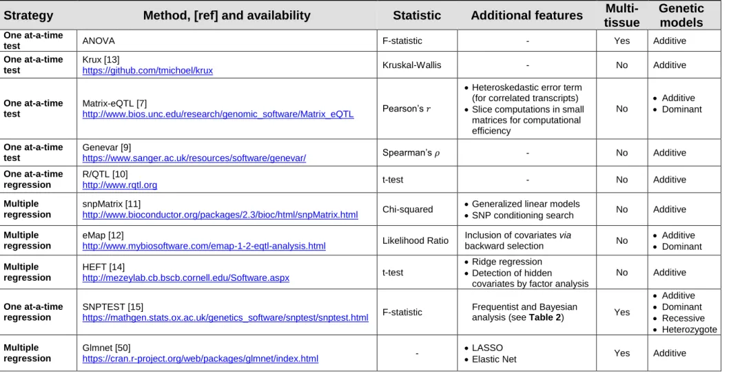
A concise list of the most commonly used frequentist eQTL mapping methods and their software implementation is reported in Table 1.
Table 1. Frequentist eQTL mapping approaches
Strategy Method, [ref] and availability Statistic Additional features
Multi-tissue
Genetic models One at-a-time
test ANOVA F-statistic - Yes Additive
One at-a-time test
Krux [13]
https://github.com/tmichoel/krux Kruskal-Wallis - No Additive
One at-a-time test
Matrix-eQTL [7]
http://www.bios.unc.edu/research/genomic_software/Matrix_eQTL Pearson’s 𝑟
Heteroskedastic error term (for correlated transcripts) Slice computations in small
matrices for computational efficiency No Additive Dominant One at-a-time test Genevar [9]
https://www.sanger.ac.uk/resources/software/genevar/ Spearman’s 𝜌 - No Additive
One at-a-time regression
R/QTL [10]
http://www.rqtl.org t-test - No Additive
Multiple regression
snpMatrix [11]
http://www.bioconductor.org/packages/2.3/bioc/html/snpMatrix.html Chi-squared
Generalized linear models
SNP conditioning search No Additive
Multiple regression
eMap [12]
http://www.mybiosoftware.com/emap-1-2-eqtl-analysis.html Likelihood Ratio
Inclusion of covariates via
backward selection No Additive Dominant Multiple regression HEFT [14] http://mezeylab.cb.bscb.cornell.edu/Software.aspx t-test Ridge regression Detection of hidden
covariates by factor analysis
No Additive
One at-a-time regression
SNPTEST [15]
https://mathgen.stats.ox.ac.uk/genetics_software/snptest/snptest.html F-statistic
Frequentist and Bayesian
analysis (see Table 2) Yes
Additive Dominant Recessive Heterozygote Multiple regression Glmnet [50] https://cran.r-project.org/web/packages/glmnet/index.html - LASSO
3. Bayesian eQTL mapping
Bayesian methods are becoming increasing popular in modern genetics [51], possibly as a consequence of recent more efficient algorithmic/computational implementations, cheaper high-performance computing solutions, and in general less computational constraints in their genome-wide applications. Unlike frequentist approaches, which try to infer the value of fixed models parameters from random data, in Bayesian inference the data are treated as a fixed quantity (since there is no randomness after observing the data) while the parameters are treated as random variables. This allows researchers to assign to parameters (and models) probabilities, making the inferential framework more intuitive and straightforward. Here we introduce a few general concepts that are at the core of the Bayesian paradigm. Denoting the parameters by 𝜃 and the observed data by 𝐷, the Bayes theorem allows to write:
𝜋(𝜃|𝐷) =ℓ(𝐷|𝜃)𝜋(𝜃)
ℓ(𝐷) =
ℓ(𝐷|𝜃)𝜋(𝜃)
∫ ℓ(𝐷|𝜃)𝜋(𝜃)𝑑 𝜋 ,
where 𝜋(𝜃|𝐷) is the posterior distribution, ℓ(𝐷|𝜃) is the likelihood
(conditionally on some parameters’ value), 𝜋(𝜃) is the prior distribution on the
parameters and ℓ(𝐷) the marginal likelihood. In a nutshell, the equation
above states that the Bayesian paradigm provides a distribution regarding what it has been learned about the parameter from the data. In contrast to the frequentist approach, where only a point estimate (Maximum Likelihood Estimation of MLE) and a standard error (SE) are obtained from the inferential process, in the Bayesian paradigm the whole distribution of the parameters is available.
Similarly, the Bayesian model selection is obtained by assigning a distribution of probability over alternative competing models and, after observing the data, selecting the most promising model as the one with the largest posterior probability. The assignment of probabilities to model parameters is made using both the information captured by the data 𝐷 and prior knowledge (or beliefs) about the structure of the model, which is encoded by the prior probability 𝜋(𝑀) of a model 𝑀. Then, a typical Bayesian experiment updates
the prior distribution 𝜋(𝑀) to the posterior 𝜋(𝑀|𝐷) by multiplying the
likelihood ℓ(𝐷|𝑀) with the prior probability of the model 𝜋(𝑀), using the Bayes theorem:
𝜋(𝑀|𝐷) =ℓ(𝐷|𝑀)𝜋(𝑀)
𝜋(𝐷) =
ℓ(𝐷|𝑀)𝜋(𝑀)
∑ ℓ(𝑖 𝐷|𝑀𝑖)𝜋(𝑀𝑖) ,
where ℓ(𝐷|𝑀) is the conditional probability of observing the data under the model and 𝜋(𝐷) is the probability of the data, which can be computed by summing over the conditionals of all possible models.
An alternative way to evaluate which model is most supported by the data 𝐷,
between two alternative models 𝑀1and 𝑀2, is to calculate the so-called Bayes
𝐵𝐹(𝑀1, 𝑀2) =ℓ(𝐷|𝑀1) ℓ(𝐷|𝑀2)= 𝜋(𝑀1|𝐷) 𝜋(𝑀1) 𝜋(𝑀2|𝐷) 𝜋(𝑀2) = 𝜋(𝑀1|𝐷) 𝜋(𝑀2|𝐷) 𝜋(𝑀1) 𝜋(𝑀2)
which is the ratio between posterior odds 𝜋(𝑀1|𝐷)/𝜋(𝑀2|𝐷) and prior odds
𝜋(𝑀1)/𝜋(𝑀2). The BF can also be interpreted as a Likelihood Ratio test
between two competing models 𝑀1and 𝑀2 when all the uncertainty about
nuisance parameters 𝜂 (i.e., parameters that are of no direct interest but are specified in the model) have been marginalised (integrated) out
ℓ(𝐷|𝑀1)
ℓ(𝐷|𝑀2)=
∫ ℓ(𝐷|𝑀1, 𝜂)𝜋(𝜂)𝑑𝜂
∫ ℓ(𝐷|𝑀2, 𝜂)𝜋(𝜂)𝑑𝜂
without conditioning as in frequentist approaches.
In Bayesian eQTL mapping the observed data typically include a 𝑛 × 1 vector of outcomes 𝑦 (i.e., gene expression levels) and a 𝑛 × 𝑝 matrix of predictor variables 𝑋 (i.e., genetic markers). The set of model parameters, their prior distribution and hence the joint posterior distribution may vary between approaches [53]. The Bayesian models presented here attempt to infer the
posterior distribution of the vector of regression coefficients 𝛽 = (𝛽1, … , 𝛽𝑝)𝛵,
which encodes the effect of markers to the gene expression level, i.e., the eQTLs.
(a) Univariate regression models
One class of Bayesian eQTL approaches associates the outcome with one
marker “at-a-time”, by computing the BF for each SNP (instead of the
frequentist p-value) [15, 19, 20, 54]. This approach is computationally efficient
since only two alternative models 𝑀1 and 𝑀2 are compared each time, i.e., 𝑀1
and 𝑀2, encoding for the inclusion/exclusion of the marker, respectively. In
this framework the BF is further simplified
𝐵𝐹(𝑀1, 𝑀2) = 𝜋(𝑀1|𝐷)
1 − 𝜋(𝑀1|𝐷)
1 − 𝜋(𝑀1)
𝜋(𝑀1) ,
where 𝜋(𝑀1) and 𝜋(𝑀1|𝐷) are the prior and posterior probability, respectively,
that the marker is an eQTL. Markers whose BF exceeds a certain threshold are therefore defined as eQTL (the general criteria for setting the optimal BF threshold based on number of predictors can be found in [15, 55]). Beyond setting the BF threshold, it has been shown that using the BF is superior to
conventional p-value since the Bayesian-inferred associations can benefit
from the elicitation of “biologically primed” informative priors [56, 57], which in some cases can improve power [58].
SNPTEST [59] performs a single-marker eQTL association analysis, i.e., implementing a “one at-a-time” strategy, which incorporates both frequentist and Bayesian association tests. In its Bayesian form, SNPTEST fits a linear
regression model that computes the posterior odds of including marker 𝑗 in
distributed 𝜀~𝛮(0, 𝜎2) , while the model parameters 𝛽, 𝜎2 are given a conjugate Normal-Inverse-Gamma prior set-up. This regression approach can be extended to map eQTL under dominant or recessive inheritance models: the prior distributions remain the same, but the genotype vector is modified and recoded to reflect dominant or recessive inheritance model. A normal
prior is used on 𝛽 with larger variance, reflecting the assumption that
dominant or recessive alleles contribute differently to the phenotypic (i.e., gene expression) variance.
(b) Bayesian Variable Selection methods
Initially, most “one at-a-time” Bayesian strategies were applied to GWAS of clinical traits or disease, in which the phenotype (disease trait) was analyzed against a genome-wide panel of genetic predictors (SNPs). When applied to these data and especially to data problem that is typical of eQTL mapping
(i.e., large number of both expression phenotypes and genetic markers),
these methods display similar problems as the simple frequentist models described in Section 2; namely, an inflated number of false positive associations and loss of power due to setting arbitrary study-wide significance thresholds [60].
Similarly to penalized-regression models, Bayesian Variable Selection (BVS) methods have been developed for eQTL mapping to analyze jointly the whole set of markers. However, differently from penalized-regression, BVS is able to perform model choice (select the markers that are likely to influence the expression of the gene) and provide parameters estimate (the regression coefficients of the active markers) at the same time [16–18, 61–65]. With both these quantities available, genome-wide significance can be obtained by controlling the FDR level [66]. Here, we describe the major components of BVS and introduce a few computational implementations of this class of approaches.
BVS - Prior set-up: similar to penalized-regression methods, BVS models try to choose few important markers with large effects. Unlike LASSO-type regressions, in BVS sparsity is not only controlled by the prior distribution on
the regression coefficients (i.e., the Lp-norm penalty in the frequentist
approach), but by specifying an a priori number of eQTLs encoded in a latent
binary vector 𝛾 = (𝛾1, … , 𝛾𝑝)𝑇, where 𝛾
𝑗 = 1 if 𝛽𝑗 ≠ 0 and 𝛾𝑗 = 0 if 𝛽𝑗 = 0. In a
nutshell, BVS can control both the level of shrinkage and the number of
non-zero eQTL effects that can be detected. These two tasks are tightly connected in BVS given the prior specification of the regression coefficients [67]:
𝛽|𝛾, 𝜎2~𝑁 (0, 𝑔𝜎2(𝑋
𝛾𝑇𝑋𝛾)
𝜆 ).
The equation above states that for the selected markers, i.e., for markers with
𝛾𝑗 = 1 since 𝛽𝑗 ≠ 0, the prior distribution on vector of regression coefficients is
normal distributed and centered in zero. The covariance matrix can be the unit diagonal matrix, giving rise to the so-called independent prior, if 𝜆 = 0 or the inverse of the covariance matrix which characterize the so-called g-prior if 𝜆 =
−1, multiplied by a constant 𝑔 and the residual variance 𝜎2. Under this
𝜀~𝛮(0, 𝜎2), where 𝛾, the vector of binary values indicating which markers are selected and therefore their number, receives a Binomial prior distribution
𝜋(𝛾) = 𝐵𝑖𝑛(𝑝, 𝜃)
where 𝜃 can be a fixed parameter or a further level of hierarchy can be
specified [1]. The prior distribution for the model parameters 𝛽, 𝜎2 usually
follows a Normal-Inverse-Gamma set-up [16, 17, 21] with a different
specification for the power-prior 𝜆. The choice of 𝜆 = −1 is particularly
appealing in eQTL studies since an a priori g-prior “discourages” highly
collinear predictors to enter the models simultaneously by inducing a negative correlation between the coefficients, therefore controlling LD structure automatically. On the opposite side with 𝜆 = 0, the regression coefficients are a priori mutually independent [59] although, given the influence of the likelihood, this does not hold a posteriori. It turns out that a priori independent prior is less capable in handling intricate correlations between markers, but its use is encouraged because it induces, like the ridge estimator, an absolute shrinkage to the regression coefficients, i.e., it shrinks greatly in directions of
small eigenvalues, whereas the g-prior proportional shrinkage retains much
more of the OLS estimator in ill-conditioned directions [68].
The specification of the prior distribution for the model parameters 𝛽, 𝜎2 is an
active area of research in Bayesian statistics, since different prior set-ups imply different levels of shrinkage. Sparsity-inducing prior set-ups include the Laplace prior [69], the spike-and-slab priors [62, 63], the horseshoe shrinkage prior [70] and local adaptation priors [17, 64] – analyzing the different features of these set-ups in detail goes beyond the scope of this review. However, here we mention that in the piMASS eQTL mapping method [17] a novel prior set-up is used on the expected genetic effect sizes linking them with the model size. In particular, the effect size prior demonstrates the biologically primed idea that if the model size is small, then the few associated markers will have large effect sizes – the opposite is expected when then model size is large. This exemplifies how the Bayesian setting can effectively leverage “biologically informed” priors to improve ad refine eQTL detection.
BVS - Model selection and posterior computation: in typical genomics and
eQTL mapping experiments the number of predictor variables is too large to
enumerate all possible combinations of latent binary vector 𝛾. Therefore
search algorithms are used to explore the model space. Most methods use Markov Chain Monte Carlo (MCMC) [17, 18, 62–64], a sampling technique in
which the posterior distribution 𝜋(𝛾|𝐷) is simulated using Markov Chain
algorithms. The idea behind is that not all the 2𝑝 possible models (i.e.,
combination of markers) need to be simulated, since the majority of them are unable to explain the data with 𝜋(𝛾|𝐷) ≈ 0. On the contrary, it is more efficient to concentrate the markers’ space exploration on important models with large 𝜋(𝛾|𝐷). In a post-processing analysis, 𝜋(𝛾|𝐷) can be used to rank the visited models and decide which one to report. The output provided by MCMC
algorithm is very rich since the sampled distribution of 𝜋(𝛾|𝐷) is available
(apart from non-interesting models with 𝜋(𝛾|𝐷) ≈ 0). However, this comes at a price since MCMC algorithms are computational intensive and, as for frequentist penalized-regression methods, rather time consuming. If the goal
of the analysis is to report only the top visited model, alternative faster sampling algorithms based on the expectation maximization (EM) algorithm [71] have been recently proposed [72].
There is a very large literature on the MCMC sampling schemes that can be used to sample realizations of 𝜋(𝛾|𝐷). The simplest MCMC algorithm that can be implemented is the Gibbs sampling [73], which is particular suitable when spike-and-slab priors are specified for the regression coefficients [18, 62, 63]. Since spike-and-slab priors can be seen as two-point mixture distribution,
once conditioning on value of jth binary latent variable 𝛾𝑗, the posterior
distribution of the jth “spike” or the “slab” is ready available and it is relatively simple to simulate from. The drawback of this approach is that it tends to mix slowly when there are correlated predictors (e.g., in the presence of LD between the markers), since the posterior distribution of regression coefficient
for the jth predictor depends on the neighbour predictors and if a marker has
been selected, 𝛾𝑗 = 1, markers in strong LD with it will be selected as well. It
turns out that the algorithm may be stuck in a particular configuration of 𝛾 for many iterations of the MCMC algorithm (slow mixing) without being able to detect the optimal combination of predictive markers. To overcome this problem, MCMC algorithms that explore more efficiently the model space
have been proposed. For instance, using a “shotgun” stochastic search [74]
one can explore the entire neighbour of the current model and randomly pick up with a non-uniform probability a model from that list. For instance in piMASS [17], once a model has been selected, the next active marker that can be included in the model is the one that shows the (residual) highest absolute correlation with the phenotype so that correlated predictors are less likely to be included in the model. The Evolutionary Stochastic Search method [16, 61, 75, 76], which we will discuss in detail below, has been designed for a more efficient and far-reaching exploration of the model space. It runs several parallel MCMC samplers that swap information about the different configurations of markers selected in each chain and therefore avoiding the slow mixing phenomenon described above.
BVS - Posterior summary and interpretation: a large number of MCMC
iterations are generally required in order to match the frequency a particular model has been sampled, 𝜋̂(𝛾|𝐷), with the theoretical posterior probability of
that model, 𝜋(𝛾|𝐷). In that case the algorithm is said to have reached
convergence. From a practical point of view, assessing convergence of MCMC is not easy and many diagnostic measures can be applied to detect any anomalous behavior of the algorithm. Moreover the initial draws of the algorithm (burn-in phase) are usually discarded because it may be possible that the models are sampled with the wrong frequency compared with the
correct theoretical probability with some models over-represented or vice
versa during the initial phase. All the models visited by the search algorithm after the burn-in are kept and summarized into a marginal posterior probability
of inclusion (MPPI) 𝜋̂(𝛾𝑗 = 1|𝐷, 𝛾\𝑗), which indicates the frequency the jth
marker has been selected in the models visited by the search algorithm. Despite its straightforward interpretation (MPPI = the probability that the
marker j explains the variation of the gene expression given all other
of it with respect to effect size or for controlling the FDR. However the classification of the MPPI into two groups will allow the assessment of their genome-wide significance. Specifically, one can employ the EM algorithm to fit a mixture of two beta distributions and then use the classification probabilities to derive the FDR, as described in [78]. Alternatively, versatile R packages that can estimate local (tail-area) FDR from the posterior distribution [79], are also available [80].
piMASS [17] is a BVS algorithm for eQTL mapping with a new regression
coefficients’ prior variance that allows either models with a large number of predictors with a small proportion of variance explained (PVE) or a small number of predictors with a large PVE. This prior set-up is in tune with what is
expected in typical eQTL mapping experiments, where few cis-eQTLs are
present with large effects and large PVE, whereas many trans-eQTLs have
relatively smaller effects and smaller PVE. Its implementation is based on a single MCMC chain with a sampling strategy that explores models made by faraway and/or uncorrelated genetic markers.
Another BVS algorithm is Evolutionary Stochastic Search (ESS) [16, 21, 61, 76] in which the level of sparsity can be controlled directly by the user
specifying the a priori expected number of predictors to be included in the
model and its variance. Moreover given the prior structure on the regression
coefficients that can be thought as a mixture of g-priors and an
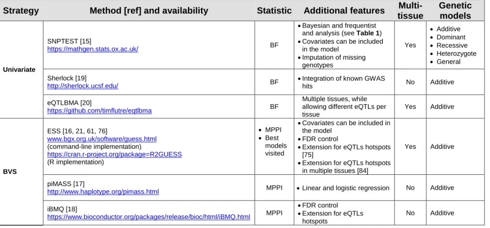
Inverse-Gamma prior [81], the level of proportional shrinkage automatically adapts to different real data scenarios. ESS uses an advanced stochastic search algorithm in which multiple models are explored by parallel MCMC samplers. Specifically, at each iteration, each chain locally selects a different model using local moves based on the Gibbs sampler [73] or a fast version of the Metropolis-Hasting algorithm [82]. Global moves, which allow the exchange of information between parallel chains about the models selected, are also implemented, using a MCMC version of genetic algorithms [83]. The combination of local and global moves allows the efficient exploration of the model space and prevents the algorithm from getting stuck to a sub-optimal model made by highly correlated predictors (i.e., genetic markers in high LD). A concise list of the most commonly used Bayesian eQTL mapping methods and their software implementation is reported in Table 2.
Table 2. Bayesian eQTL mapping approaches
Strategy Method [ref] and availability Statistic Additional features
Multi-tissue Genetic models Univariate SNPTEST [15] https://mathgen.stats.ox.ac.uk/ BF
Bayesian and frequentist and analysis (see Table 1) Covariates can be included
in the model Imputation of missing genotypes Yes Additive Dominant Recessive Heterozygote General Sherlock [19] http://sherlock.ucsf.edu/ BF
Integration of known GWAS
hits No Additive
eQTLBMA [20]
https://github.com/timflutre/eqtlbma BF
Multiple tissues, while allowing different eQTLs per tissue Yes Additive BVS ESS [16, 21, 61, 76] www.bgx.org.uk/software/guess.html (command-line implementation) https://cran.r-project.org/package=R2GUESS (R implementation) MPPI Best models visited
Covariates can be included in the model
FDR control
Extension for eQTLs hotspots [75]
Extension for eQTLs hotspots in multiple tissues [84]
Yes Additive
piMASS [17]
http://www.haplotype.org/pimass.html MPPI Linear and logistic regression No Additive iBMQ [18]
https://www.bioconductor.org/packages/release/bioc/html/iBMQ.html MPPI
FDR control
Extension for eQTLs hotspots
4. Multi-tissue extensions
Transcriptomic studies can assess gene expression levels in multiple tissues or cell-types in order to understand the mechanism of gene regulation at the systems-level, including mapping of eQTLs in multiple systems [85]. While expression of certain genes and pathways can be conserved across different tissues, intersecting results from several single-tissue eQTL analyses (for instance by imposing the same FDR threshold in each eQTL study) may be too conservative and can lead to inflated false negative rate [84]. In contrast, utilizing a cross-tissue analysis of eQTLs by jointly mapping gene expression profiles from multiple tissues, has been shown to increase power to detect small effect eQTLs (specifically, trans-eQTLs) [20–22].
Several eQTL mapping approaches, including some discussed above, have been extended to allow eQTL mapping of tissue-consistent QTLs (i.e., eQTLs that are detected across multiple tissues), by allowing BVS models to analyze
multivariate outcomes. Thus, assuming an experiment with 𝑛 samples, 𝑝
predictors and 𝑞 outcomes (tissues or cell-types), the multiple outcome linear regression model can be written as:
𝑌 = 𝐴 + 𝑥1𝐵1+ ⋯ + 𝑥𝑝𝐵𝑝+ 𝐸, 𝐸~𝑀𝑁(0, 𝐼𝑛, 𝛴),
where 𝑌 is a 𝑛 × 𝑞 matrix of outcomes, 𝐴 is a 𝑛 × 𝑞 matrix of intercepts, 𝑥𝑗 is
the jth predictor encoded in a 𝑛 × 1 vector and 𝐵𝑗 = (𝛽𝑗,1, … , 𝛽𝑗,𝑞) is the vector
of regression coefficients that links the jth predictor with the multiple outcomes 𝑌. Finally, 𝐸 is the 𝑛 × 𝑞 matrix of errors that is distributed as a matrix-variate
normal distribution centered in zeros, with the matrix 𝛴 that controls the
residual correlation between the 𝑞 outcomes.
The above equation can be seen as the multiple-outcome extension of the linear model and both SNPTEST [15] and ESS [21, 76] come with this multivariate outcome extensions. Both algorithms use a similar prior set-up,
modeling the matrix of regression coefficients 𝐵 = (𝐵1, … , 𝐵𝑝)
𝑇
by a
matrix-variate normal prior |𝛴~𝛭𝛮 (𝑔(𝑋𝛾𝑇𝑋𝛾)
𝜆
, 𝛴), where (𝑋𝛾𝑇𝑋𝛾)
𝜆
is the correlation matrix between the selected markers with 𝜆 = 0 in SNPTEST and 𝜆 = −1 in ESS and 𝛴 is the 𝑞 × 𝑞 matrix modelling the correlation between outcomes (i.e., gene expression levels in different tissues). The model is further
specified by placing an Inverse-Wishart prior on 𝛴, 𝛴~𝐼𝑊(𝑐, 𝑄), where 𝑐
indicates the degrees of freedom and 𝑄 is proportional to the expected
residual variance. eQTLBMA [20] is another eQTL mapping method that is designed to handle multi-tissue eQTLs, again using a matrix-variate normal
prior set-up – but it also uses a hierarchical model which permits
heterogeneity between tissues, to allow the estimate of genetic effects both between- and within-tissues.
Frequentist approaches for multiple-tissue eQTL analysis have also been implemented: for example the multivariate version of the ANOVA model (MANOVA) or the Wilks’ test statistic [86], a generalization of the F-statistic for multivariate random variables [87]. Multiple-outcome penalized-regression approaches have also been proposed [43, 88], while the R package glmnet [50] includes options that fit multiple-outcome Gaussian models. However,
controlling for FWER and FDR is more challenging than in the case of univariate penalized linear regression, and extensions of stability selection [47] for the multivariate problem are still in the stage of development. As a result, interpretation of the multi-tissue eQTL results from multivariate penalized-regression has to be based on the value of regression coefficients, and so thresholding can be a challenge.
5. Empirical comparison of frequentist and Bayesian eQTL mapping In this section we present an illustrative example of previously reported eQTL
mapping for the Hopx gene, which in the rat has been shown to be under
control by two loci on chromosome 14 (cis-eQTL) and chromosome 2
(trans-eQTL), respectively; where both cis- and trans-eQTLs have been
experimentally validated [21]. Rather than providing a comprehensive comparison of eQTL mapping methods (systematic simulation studies that compare methods in a variety of scenarios can be found in [76]), our purpose here is to use this empirical eQTL mapping example to facilitate discussion on the comparison between frequentist and Bayesian eQTL mapping approaches. In this eQTL mapping exercise, we have used microarray gene
expression data for the Hopx gene in two tissues (heart and fat) from 29
recombinant inbred (RI) rat strains (generated by sibling-mating the offspring of a genetic cross until the progenies are inbred), genotyped at 1,307 SNPs. Since rats within an RI strain have complete homozygosity at each locus in the genome, each genetic marker allows splitting the rat population in two
groups. We considered (i) a single-tissue example using gene expression
data from the heart only and (ii) a multi-tissue example using gene expression data from both tissues.
(i) Single-tissue example
We mapped genome-wide eQTLs for the heart gene expression data using three frequentist (Matrix-eQTL [7], Kruskal-Wallis test [8] and LASSO from the R package glmnet [50]) and three Bayesian methods (SNPTEST [15], ESS
[16, 61], piMASS [17]) - see Tables 1-2 for reference. The parameters and
eQTL analysis details are provided in the table below and the eQTL results from all methods are reported in Figure 1.
Method Genome-wide eQTL analysis details
Matrix-eQTL We used the linear additive model as the genotypes are binary. p-values were
adjusted using the Benjamini-Yekutieli FDR method [89]. We selected eQTL associations at 1% FDR.
Kruskal-Wallis test
The test is the non-parametric equivalent of a one-way ANOVA. We used the kruskal.test function in R to extract p-values, and selected eQTLs
at 1% FDR employing Benjamini-Yekutieli method.
Glmnet-LASSO
We performed 9-fold cross-validation using the function cv.glmnet, setting alpha = 1 and family = “gaussian”. After obtaining estimates on the regression coefficients, these were transformed in posterior probabilities by using stability selection method, implemented in the R package stabs [90]. We declared significance with a threshold of 0.2 on the posterior probabilities.
SNPTEST We ran the Bayesian version of SNPTEST-v.2.5.2 with 𝛽~𝛮(0,0.02𝜎2), 𝜎2~𝐼𝐺(3,2) as priors (prior_qt_mean_b 0 prior_qt_V_b 0.02 prior_qt_a 3
-prior_qt_b 2). We called eQTLs at log10𝐵𝐹 ≥ 0.25.
piMASS We ran piMASS-v.0.90 setting the prior probability that a SNP is truly
associated with the phenotype to range between 1 and 56 (-pmin 1 –pmax 56) and the model size to range from 1 to 100 (-smin 1 –smax 100). We did not impose constraints on the hyperparameter ℎ and to the minor allele frequency (-exclude_maf 0). The burn-in phase was set to 106 iterations, followed by 107
sampling iterations, while only one every 10 models considered by the sampling steps was recorded (-w 1,000,000 –s 10,000,000 –num 10). We computed the FDR on the marginal posterior probabilities of inclusion (MPPI) by fitting a mixture of beta distributions, as described in [91].
ESS We ran GUESS-v.1.1, setting the a priori expected model size to 𝐸 = 5, 𝑆 = 3
Egam 5 –Sgam 3) and ran 25,000 steps of which the first 5,000 as burn-in (-nsweep 25,000 –burn_in 5,000). We computed FDR on the MPPI provided by ESS in the same way as described above for piMASS algorithm.
All six approaches detected a clear cis-QTL signal on rat chromosome 14
(close to the location of Hopx gene), although for the ANOVA and SNPTEST the level of significance reached at the cis-eQTL is only a little higher than the rest of the genome. In this example, Glmnet-LASSO and ESS are the only
methods that unambiguously detect a trans-eQTL signal on chromosome 2.
However, Glmnet-LASSO is also picking an additional eQTL signal on chromosome 3. Therefore, in this example, the classic method that implements penalization (Glmnet-LASSO) and one of the Bayesian approaches that uses sparsity (ESS), show good performance in detecting both the cis- and trans-eQTL signals (however, Glmnet-LASSO is also picking an comparable eQTL signal on chromosome 3). The most striking observation that we can derive from this empirical analysis is that widely used frequentist methods (e.g., Matrix-eQTL) which employ a “one at-a-time” strategy were not able to detect the trans-eQTL signal on rat chromosome 2 (with both the cis-
and trans-eQTL signals experimentally validated, as previously reported in
[21]), therefore highlighting an important limitation of this approach. (ii) Multiple-tissue example
For the second illustrative example, we ran multivariate ANOVA,
Glmnet-LASSO and ESS to jointly map eQTLs for Hopx gene expression levels
across heart and fat tissues from the 29 rat RI strains used for single-tissue eQTL analysis. The parameters and eQTL analysis details are provided in the table below and the eQTL results in heart and fat tissues from all methods are reported in Figure 2.
Method Genome-wide eQTL analysis details
MANOVA We ran a Wilks’ test using the R function wilks.test setting method = “rank”,
and selected associations at 1% FDR employing Benjamini-Yekutieli method.
Glmnet-LASSO
We set parameters to cv.glmnet in the same way as in the single-tissue analysis, but specified family = “mgaussian” to perform multivariate analysis.
ESS The prior set-up was the same as in single-tissue analysis described in the table above, but we instead ran 110,000 sampling steps, of which 10,000 were burn-in. No further specification for multi-outcome analysis is required by ESS
that automatically recognises the multivariate nature of the matrix 𝑌.
Similarly to the results of eQTL analysis in the single tissue, all three methods
unambiguously identified a strong cis-effect on rat chromosome 14, which
therefore suggests the presence of a common cis-eQTL in heart and fat
tissues. However, only the Glmnet-LASSO and ESS methods were able to
identify an additional trans-eQTL on rat chromosome 2, suggestive of
common trans-regulation between the two tissues (as previously shown for
other trans-eQTL signals conserved across multiple tissues in this genetic
system [91]). Glmnet-LASSO identifies the two eQTLs without identifying
false-positives, although the signal from the trans-effect is much weaker than that of the cis-effect. One important issue with Glmnet-LASSO is in the output provided by the algorithm: although the regression coefficients of the selected markers for the two tissues are clearly reported there is not a simple way to combine them and to transform the tissue-specific effects into a posterior probability, for instance, by the stability selection procedure. In the same eQTL example ESS picks up with a very low MPPI an additional signal from chromosome 10, which is likely to be a false positive. A noteworthy observation that can be derived from the results of the ESS analysis is that the MPPI of the trans-effect is almost doubled in multiple-tissues compared to the single tissue analysis, highlighting the advantage of combining information from multiple sources (in this case tissues). From a biological viewpoint, when
compared the MPP of the same trans-eQTL detected in the single-tissue
analysis (Figure 1), the signal in the multi-tissue maybe reflects a potential pleiotropic nature of this eQTL.
6. Discussion and outlook
We discussed the challenges in eQTL mapping and reviewed several commonly used approaches, including their advantages and advantages. In particular, we emphasized the useful features provided by the Bayesian methods. Using a simple yet informative example of polygenic regulation of gene expression in the rat, we illustrated the major differences between frequentist and Bayesian eQTL mapping approaches. In this, we first focused
on single-tissue eQTL mapping (Figure 1), where both cis- and trans-signals
have been previously experimentally validated [21]. We used this demonstrative example to show that frequentist approaches based on a computational efficient strategy that tests for association all transcript-marker pairs (“one at-a-time”) were not suitable to detected polygenic control of gene expression. In contrast, methods based on multivariate models, either frequentist (LASSO) or Bayesian (ESS), were able to detect both eQTLs, although ESS performed marginally better as it eliminated possible false positive associations identified by the LASSO-based approach. We then extended this example to include gene expression data from two tissues for the same gene: the eQTL results were very similar to what observed in the two single tissue cases, with the Bayesian variable selection method detecting
unambiguously both cis- and trans-eQTLs (Figure 2). This example also
highlighted the benefits of using multiple tissues for simultaneous eQTL mapping since, by joint modelling the dependence between tissues, it further
single-tissue experiment [20–22].
For Bayesian approaches, the ability to handle the whole set of predictors (genome-wide genetic markers) and model their correlation (i.e., accounting for LD structure) as well as providing the whole posterior distribution of the parameters come at a price. The more traditional (frequentist) eQTL approaches (such as Matrix-eQTL [7]) have the attractive feature of computational efficiency compared to the more demanding BVS methods. This might account for the common application of frequentist eQTL mapping methods in biomedical research. However, as highlighted in our illustrative examples, the high computational efficiency of frequentist approaches might come at the expenses of missing polygenic control of gene expression. This
can have important implications when both cis- and trans-eQTLs are
investigated at the genome-wide level, usually resulting in a smaller fraction of
“replicable” trans-eQTLs as compared with cis-eQTLs, and advocating the
use of larger populations to boost detection of small trans-effects [92].
However, recent advancements in high-performance computing have rendered the application of MCMC methods feasible even for hundreds of
thousands of predictors in hundreds (if not thousands) of individuals [76] –
which now justifies the increasing popularity of the Bayesian eQTL mapping methods. In contrast, although recent advances in the computational aspects of the LASSO solution [93], frequentist penalized-regression methods still need time-consuming cross-validation procedure to estimate the penalty parameter 𝜆. In the case of Elastic Net a two-dimensional grid is required in
order to select the optimal 𝜆1, 𝜆2 penalties. Selecting the optimal parameters
however, necessitates a very fine-grained grid of penalties to be analyzed, which is even more computationally expensive.
Regarding interpretation of the eQTL results, in BVS approaches all the models visited by the search algorithm (after the burn-in) are kept and summarized into a marginal posterior probability of inclusion (MPPI). Penalized-regression models usually output estimates of regression coefficient values, which can vary largely between experiments and therefore are less safe for declaring eQTL associations consistently across studies. Moreover, estimation of the FDR from the regression coefficients is not possible, so one is limited to controlling family-wise error rates, a more conservative approach that can lead to false negatives. In contrast, several techniques that control the FDR from the MPPI are now available, making the genome-wide control of the significance level less of a problem for Bayesian eQTL methods. In addition, although not directly investigated in our illustrative examples, the Bayesian prior set-up offers more flexibility to consider (and explore) different eQTL models, for example by specifying the number of expected eQTLs and their effect size or by using genomic locations of the transcripts to improve the accuracy of the posterior distribution for the location of the eQTL [94].
In summary, we advocate that Bayesian approaches are in general more flexible to analyze complex genetic regulation of expression than frequentist methods. In particular, Bayesian eQTL mapping strategies can adapt naturally to a wider range of applications, such as (i) detection of polygenic effects on gene expression [21], (ii) epistatic eQTL interactions [63], (iii) eQTLs hotspots
[75] and (iv) eQTLs and eQTLs hotspots across multiple-tissues [21, 75, 84]. We also argue that using Bayes Factors might provide a more objective way to call statistically significant eQTLs [55, 95] and compare them across
studies. Conversely, using computationally inexpensive p-values generated
by frequentist approaches to call significant eQTLs requires a threshold for genome-wide significance that can varies largely with sample size as well as with other study-specific factors. While this issue is well known and yet often
ignored, it is likely to be highly relevant to the development of reference eQTL
databases and resources. Since eQTL analyses have been proved useful in the identification of molecular pathways affecting disease susceptibility, e.g., [6, 91, 96, 97], it is generally advisable to use truly multivariate eQTL mapping strategies that can provide more flexibility in modeling complex data structures and can have enhanced interpretability of the results. In this respect, Bayesian mapping approaches now provide a valid alternative to traditional “one at-a-time” frequentist methods and a richer and easy to interpret output than penalized-regression methods.
Figure legends
Figure 1. For each SNP genotyped in the rat genome (x-axis), for each
method we report the evidence in support of genetic regulation of Hopx gene
expression in the heart tissue (y-axis). The input consisted of 𝑛 × 1
expression values and a 𝑛 × 𝑝 matrix of predictors (genome-wide SNPs),
where 𝑛 = 29 and 𝑝 = 1,307. Black dots, associations called at 1% FDR.
Boxes highlight the chromosomal locations where the cis- and trans-eQTLs
are located, respectively.
Figure 2. For each SNP genotyped in the rat genome (x-axis), for each
method we report the evidence in support of genetic regulation of Hopx gene
expression simultaneously in the heart and fat tissues (y-axis). The input consisted of 𝑛 × 2 expression values (fat and heart, respectively) and a 𝑛 × 𝑝
matrix of predictor variables (genome-wide SNPs), where 𝑛 = 29 and 𝑝 =
1,307. Black dots, associations called at 1% FDR. For the Glmnet-LASSO,
the blue and black dots indicate the absolute values of β-coefficients
estimated in fat and heart tissues, respectively. Boxes highlight the
chromosomal locations where the cis- and trans-eQTLs are located,
Acknowledgments
We acknowledge funding from Medical Research Council Grant G 1002319 (L.B.), MR/M013138/1 (L.B.), MR/M004716/1 (M.I. and E.P.) and Duke-NUS Graduate Medical School Singapore (E.P.).
References
1. Guo H, Fortune MD, Burren OS, et al. (2015) Integration of disease
association and eQTL data using a Bayesian colocalisation approach highlights six candidate causal genes in immune-mediated diseases. Hum Mol Genet 24:3305–13. doi: 10.1093/hmg/ddv077
2. Pierce BL, Tong L, Chen LS, et al. (2014) Mediation analysis
demonstrates that trans-eQTLs are often explained by cis-mediation: a genome-wide analysis among 1,800 South Asians. PLoS Genet
10:e1004818. doi: 10.1371/journal.pgen.1004818
3. Kang H, Kerloc’h A, Rotival M, et al. (2014) Kcnn4 is a regulator of
macrophage multinucleation in bone homeostasis and inflammatory disease. Cell Rep 8:1210–24. doi: 10.1016/j.celrep.2014.07.032
4. Rotival M, Zeller T, Wild PS, et al. (2011) Integrating genome-wide
genetic variations and monocyte expression data reveals trans-regulated gene modules in humans. PLoS Genet 7:e1002367. doi: 10.1371/journal.pgen.1002367
5. Fehrmann RSN, Jansen RC, Veldink JH, et al. (2011) Trans-eQTLs
reveal that independent genetic variants associated with a complex phenotype converge on intermediate genes, with a major role for the HLA. PLoS Genet 7:e1002197. doi: 10.1371/journal.pgen.1002197
6. Small KS, Hedman AK, Grundberg E, et al. (2011) Identification of an
imprinted master trans regulator at the KLF14 locus related to multiple metabolic phenotypes. Nat Genet 43:561–4. doi: 10.1038/ng.833
7. Shabalin A a (2012) Matrix eQTL: ultra fast eQTL analysis via large
matrix operations. Bioinformatics 28:1353–8. doi: 10.1093/bioinformatics/bts163
8. MacDonald JH (2009) Kruskal-Wallis Test. Biol Handb Stat 165–172.
doi: 10.1002/9780470479216.corpsy0491
9. Yang T-P, Beazley C, Montgomery SB, et al. (2010) Genevar: a
database and Java application for the analysis and visualization of SNP-gene associations in eQTL studies. Bioinformatics 26:2474–2476. doi: 10.1093/bioinformatics/btq452
10. Broman KW, Wu H, Sen S, Churchill GA (2003) R/qtl: QTL mapping in experimental crosses. Bioinformatics 19:889–90.
11. Clayton D, Leung H-T (2007) An R Package for Analysis of Whole-Genome Association Studies. Hum Hered 64:45–51. doi:
12. Sun W (2009) eQTL Analysis by Linear Model. In: http://www.bios.unc.edu/~weisun/software/eMap.pdf.
http://www.bios.unc.edu/~weisun/software/eMap.pdf. Accessed 20 Oct 2015
13. Qi J, Asl HF, Björkegren J, Michoel T (2014) kruX: matrix-based non-parametric eQTL discovery. BMC Bioinformatics 15:11. doi:
10.1186/1471-2105-15-11
14. Gao C, Tignor NL, Salit J, et al. (2014) HEFT: eQTL analysis of many thousands of expressed genes while simultaneously controlling for hidden factors. Bioinformatics 30:369–76. doi:
10.1093/bioinformatics/btt690
15. Marchini J, Howie B, Myers S, et al. (2007) A new multipoint method for genome-wide association studies by imputation of genotypes. Nat Genet 39:906–13. doi: 10.1038/ng2088
16. Bottolo L, Chadeau-hyam M, Hastie DI, et al. (2011) ESS++: A C++ objected-oriented algorithm for Bayesian stochastic search model exploration. Bioinformatics 27:587–588. doi:
10.1093/bioinformatics/btq684
17. Guan Y, Stephens M (2011) Bayesian variable selection regression for genome-wide association studies and other large-scale problems. Ann Appl Stat 5:1780–1815.
18. Scott-Boyer MP, Imholte GC, Tayeb A, et al. (2012) An integrated hierarchical Bayesian model for multivariate eQTL mapping. Stat Appl Genet Mol Biol. doi: 10.1515/1544-6115.1760
19. He X, Fuller CK, Song Y, et al. (2013) Sherlock: detecting gene-disease associations by matching patterns of expression QTL and GWAS. Am J Hum Genet 92:667–80. doi: 10.1016/j.ajhg.2013.03.022
20. Flutre T, Wen X, Pritchard J, Stephens M (2013) A Statistical
Framework for Joint eQTL Analysis in Multiple Tissues. PLoS Genet. doi: 10.1371/journal.pgen.1003486
21. Petretto E, Bottolo L, Langley SR, et al. (2010) New insights into the genetic control of gene expression using a Bayesian multi-tissue approach. PLoS Comput Biol 6:e1000737. doi:
10.1371/journal.pcbi.1000737
22. Sul JH, Han B, Ye C, et al. (2013) Effectively Identifying eQTLs from Multiple Tissues by Combining Mixed Model and Meta-analytic Approaches. PLoS Genet 9:e1003491. doi:
transcriptional regulation in budding yeast. Science 296:752–5. doi: 10.1126/science.1069516
24. Dudoit S, Yang YH, Callow MJ, Speed TP (2002) Statistical methods for identifying differentially expressed genes in replicated cDNA microarray experiments. Stat Sin 12:111–139. doi:
10.1146/annurev.psych.53.100901.135153
25. Gerrits A, Li Y, Tesson BM, et al. (2009) Expression quantitative trait loci are highly sensitive to cellular differentiation state. PLoS Genet 5:e1000692. doi: 10.1371/journal.pgen.1000692
26. Zhou X, Stephens M (2014) Efficient multivariate linear mixed model algorithms for genome-wide association studies. Nat Methods 11:407– 9. doi: 10.1038/nmeth.2848
27. Narahara M, Higasa K, Nakamura S, et al. (2014) Large-Scale East-Asian eQTL Mapping Reveals Novel Candidate Genes for LD Mapping and the Genomic Landscape of Transcriptional Effects of Sequence Variants. PLoS One 9:e100924. doi: 10.1371/journal.pone.0100924 28. Duggal G, Wang H, Kingsford C (2014) Higher-order chromatin
domains link eQTLs with the expression of far-away genes. Nucleic Acids Res 42:87–96. doi: 10.1093/nar/gkt857
29. Gatti DM, Shabalin AA, Lam T-C, et al. (2009) FastMap: fast eQTL mapping in homozygous populations. Bioinformatics 25:482–9. doi: 10.1093/bioinformatics/btn648
30. Benjamini Y, Hochberg Y (1995) Controlling the false discovery rate: a practical and powerful approach to multiple testing. J R Stat Soc Ser B Methodol 57:289–300. doi: 10.2307/2346101
31. (2013) The Genotype-Tissue Expression (GTEx) project. Nat Genet 45:580–5. doi: 10.1038/ng.2653
32. Hoerl AE, Kennard RW (1970) Ridge Regression: Biased Estimation for Nonorthogonal Problems. Technometrics 12:55–67. doi:
10.1080/00401706.1970.10488634
33. Tibshirani R (2011) Regression shrinkage and selection via the lasso: A retrospective. J R Stat Soc Ser B Stat Methodol 73:273–282. doi:
10.1111/j.1467-9868.2011.00771.x
34. Wu TT, Chen YF, Hastie T, et al. (2009) Genome-wide association analysis by lasso penalized logistic regression. Bioinformatics 25:714– 721. doi: 10.1093/bioinformatics/btp041
35. Zou H (2006) The Adaptive Lasso and Its Oracle Properties. J Am Stat Assoc 101:1418–1429. doi: 10.1198/016214506000000735