Multidimensional Scaling
P.J.F. Groenen1 and S. Winsberg2 1 Econometric Institute, Erasmus University Rotterdam,P.O. Box 1738, 3000 DR Rotterdam, The Netherlands email: [email protected]
2 Predisoft, San Pedro, Costa Rica email: [email protected]
Econometric Institute Report EI 2006-49
Abstract. Multidimensional scaling aims at reconstructing dissimilarities between pairs of objects by distances in a low dimensional space. However, in some cases the dissimilarity itself is not known, but the range, or a histogram of the dissimilarities is given. This type of data fall in the wider class of symbolic data (see Bock and Diday (2000)). We model three-way two-mode data consisting of an interval of dissimilarities for each object pair from each of K sources by a set of intervals of the distances defined as the minimum and maximum distance between two sets of embedded rectangles representing the objects. In this paper, we provide a new algorithm called3WaySym-Scalusing iterative majorization, that is based on an algorithm,I-Scaldeveloped for the two-way case where the dissimilarities are given by a range of values ie an interval (see Groenen et al. (2006)). The advantage of iterative majorization is that each iteration is guaranteed to improve the solution until no improvement is possible. We present the results on an empirical data set on synthetic musical tones.
Keywords: Multidimensional scaling, Three-way data, Interval data, Sym-bolic data analysis,3WaySym-Scal.
1
Introduction
Classical multidimensional scaling (MDS) models the dissimilarities among a set of objects as distances between points in a low dimensional space. The aim of MDS is to represent and recover the relationships among the objects and to reveal the dimensions giving rise to the space. To illustrate: the goal in many MDS studies, for example, in psychoacoustics or marketing is to visualize the objects and the distances among them and to discover and reveal the dimensions underlying the dissimilarity ratings, that is, the most important perceptual attributes of the objects.
Often, the proximity data available for the n objects consist of a single numerical value for the dissimilarityδij between each object pair. Then, the
data may be presented in a single dissimilarity matrix with the entry for the i-th row and the j-th column being a single numerical value represent-ing the dissimilarity between thei-th and j-th object (withi= 1, . . . , n and j = 1, . . . , n). Techniques for analyzing this two-way, one-mode data have been developed (see, e.g., Kruskal (1964), Winsberg and Carroll (1989), or Borg and Groenen (2005)). Sometimes proximity data are collected from K sources, for example, a panel of K judges or under K different conditions, yielding three-way two-mode data and ann×n×Karray of single numerical values. Techniques have been developed to deal with this form of data permit-ting the study of individual or group differences underlying the dissimilarity ratings (see, e.g., Carroll and Chang (1972), Winsberg and DeSoete (1993)). All of these above mentioned MDS techniques require that each entry of the dissimilarity matrix, or matrices be a single numerical value. However, the objects in the set under consideration may be of such a complex nature that the dissimilarity between each pair of them is better represented by a range, that is, an interval of values, or a histogram of values rather than a single value. For example, if the number of objects under study becomes very large, it may be unreasonable to collect pairwise dissimilarities from each judge and one may wish to aggregate the ratings from many judges where each judge has rated the dissimilarities from a subset of all the pairs. Then, rather than using an average value of dissimilarity for each object pair one would wish to retain the information contained in the interval or histogram of dissimilarities obtained for each pair of objects. Or, it might be useful to collect data reflecting the imprecision or fuzziness of the dissimilarity between each object pair. Then, theij-th entry in then×ndata matrix, that is, the dissimilarity between objects i and j, is either an interval or an empirical distribution of values (a histogram). In these cases, the data matrix consists of symbolic data.
By now, MDS of symbolic data can be analyzed by several techniques. The case where the dissimilarity between each object pair is represented by a range or interval of values has been treated by Denœux and Masson (2000) and Masson and Denœux (2002). They model each object as alternatively a hyperbox (hypercube) or a hypersphere in a low dimensional space and use a gradient descent algorithm. Groenen et al. (2006) have developed an MDS technique for interval data which yields a representation of the objects as hyperboxes in a low-dimensional Euclidean space rather than hyperspheres because the hyperbox representation is reflected as a conjunction ofp prop-erties wherepis the dimensionality of the space. We shall follow this latter approach here.
The hyperbox representation is interesting for two reasons. First a hyper-box is more appealing because it allows a strict separation between the units of the dimensions it uses. For example, the top speed of a certain type of car might be between 170 and 190 km/h and its fuel consumption between 8 and 10 liters per 100 km. These aspects can be easily described alternatively as
an average top speed of 180 km/h plus or minus 10 km/h and an average fuel consumption of 9 liters per 100 km plus or minus 1. Both formulations are in line with the hyperbox approach. However, the hypersphere interpretation would be to state that the car is centered around a top speed of 180 km/h and a fuel consumption of 9 liters per 100 km and give a radius. The units of this radius cannot be easily expressed anymore. A second reason for using hyperboxes is that we would like to discover relationships in terms of the underlying dimensions. The use of hyperboxes leads to unique dimensions, whereas the the use of hyperspheres introduces the freedom of rotation so that dimensions are not unique anymore.
Groenen and Winsberg (2006) have extended the method developed by Groenen et al. (2006) to deal with the case in which the dissimilarity between objectiand objectjis an empirical distribution of values or, equivalently, a histogram.
All of the methods described above for MDS of symbolic data treat the two-way one-mode case. That is, they deal with a single data matrix. Here, we extend that approach to deal with the two-mode three-way case. We consider the case where each ofKjudges denote the dissimilarity between thei-th and j-th object pair as an interval, or a histogram thereby giving a range of values or a fuzzy dissimilarity. So, the accent here will be on individual differences. Of course, the method also applies to the case where data is collected forK conditions, where for each condition the dissimilarity between the i-th and j-th pair is an interval, or a histogram.
In the next section, we review briefly theI-Scalalgorithm developed by Groenen et al. (2006) for MDS of interval dissimilarities based on iterative majorization. Then, we present an extension of the method to the three-way two-mode case and analyze an empirical data sets dealing with dissimilar-ities of sounds. The paper ends with some conclusions and suggestions for continued research.
2
MDS of Interval Dissimilarities
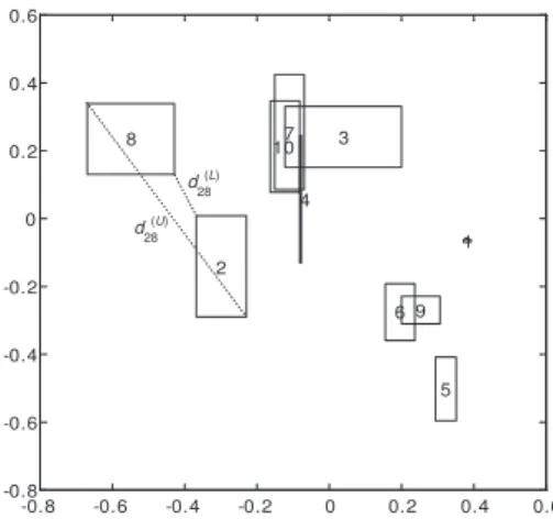
We now review briefly the case of two-way one-mode MDS of interval dissim-ilarities. In this case, an interval of a dissimilarity will be represented by a range of distances between the two hyperboxes of objects i andj. This ob-jective is achieved by representing the objects by rectangles and approximate the upper bound of the dissimilarity by the maximum distance between the rectangles and the lower bound by the minimum distance between the rect-angles. An example of rectangle representation is shown in Figure 1. It also indicates how the minimum and maximum distance between two rectangles is defined.
By using hyperboxes, both the distances and the coordinates are ranges. Let the coordinates of the centers of the rectangles be given by the rows of the n×p matrix X, where n is the number of objects and p the
dimen--0.8 -0.6 -0.4 -0.2 0 0.2 0.4 0.6 -0.8 -0.6 -0.4 -0.2 0 0.2 0.4 0.6 1 2 3 4 5 6 7 8 9 10 d 28 (L) d 28 (U)
Fig. 1.Example of distances in MDS for interval dissimilarities where the objects are represented by rectangles.
sionality. The distance from the center of rectangle i along axis s, denoted by the spread, is represented byris which is by definition nonnegative. The
maximum Euclidean distance between rectanglesiandj is given by d(U)ij (X,R) = Ã p X s=1 [|xis−xjs|+ (ris+rjs)]2 !1/2 (1) and the minimum Euclidean distance by
d(L)ij (X,R) = Ã p X s=1 max[0,|xis−xjs| −(ris+rjs)]2 !1/2 . (2)
This definition implies that rotation of the axes changes the distances be-tween the hyperboxes because they are always parallel to the rotated axes. This sensitivity for rotation can be seen as an asset because it makes a so-lution rotational unique, which is not true for ordinary MDS. In the special case ofR=0, the hyperboxes become points and the rotational uniqueness disappears as in ordinary MDS.
Symbolic MDS for interval dissimilarities aims at approximating the lower and upper bounds of the dissimilarities by minimum and maximum distances between rectangles. This objective is formalized by the I-Stress loss function
σ2 I(X,R) = n X i<j wij h δ(U)ij −d(U)ij (X,R) i2 + n X i<j wij h δ(L)ij −d(L)ij (X,R) i2 , whereδij(U)is the upper bound of the dissimilarity of objectsi andj,δ(L)ij is the lower bound , and wij is a given nonnegative weight. σI2(X,R) can be
Iterative majorization has the advantage that I-Stress is guaranteed to reduce in each iteration from any starting configuration until a stationary point is obtained. In practice, the algorithm stops at a stationary point that is a local minimum. Another important property for the purpose of this paper is that, in each iteration, the algorithm operates on a quadratic function inX
andR. Groenen et al. (2006) have derived the quadratic majorizing function forσ2
I(X,R) as the one at the right hand side of
σ2I(X,R)≤ p X s=1 (x0sA(1)s xs−2x0sB(1)s ys) + p X s=1 (r0 sA(2)s rs−2r0sb(2)s ) + p X s=1 X i<j (γijs(1)+γijs(2)), (3) wherexsis columnsofX,rsis columnsofR,ysis columnsofY(the
pre-vious estimate ofX). The matricesA(1)s ,Bs(1),A(2)s , vectorsb(2)s , and scalars
γijs(1), γijs(2) all depend dependent on previous estimates of X and R, hence they are known at the present iteration. Their exact definition can be found in Groenen et al. (2006). For our purposes, it is important to realize that the majorizing function at the right of (3) is quadratic inX andR, so that an update can be readily derived by setting the derivatives equal to zero.
Another important feature of the majorizing function being quadratic is that it becomes easy to impose the constraints that we will need for the extension to two-mode three-way symbolic MDS proposed in this paper. For more details on iterative majorization and its use in three-way MDS, see, for example, De Leeuw and Heiser (1980) and Borg and Groenen (2005).
3
Two-Mode Three-Way MDS of Interval Data
The I-Scal algorithm developed by Groenen et al. (2006) can be extended quite easily to two-mode three-way interval data. In this case, we have an interval available of the dissimilarities available for replication `= 1, . . . , L. Then,δ(L)ij` andδ(U)ij` are the lower and upper boundary of the interval ofδijfor
replication`. Of course, a normal I-Scal solution could be computed for every replication separately. However, here we impose restrictions of the weighted Euclidean model similar to the Indscal approach of Carroll and Chang (1972). The main idea is to have a single common space of hyperboxes and allow each replication ` to stretch or shrink the dimensions to fit its ranges of dissimilarities as good as possible. Let X and R denote here the centers and spreads of the hyperboxes in the common space. Then, the weighted Euclidean model restrictions imply that the hyperboxes for the individual replication`are modelled as
X` =XV` (4)
whereV`is ap×pdiagonal matrix with dimension weights for replication`.
This objective can be obtained by minimizing the 3Way-IStress loss function σ23Way(X,R,V1, . . . ,VL) = X ` n X i<j wij h
δij`(U)−d(U)ij (XV`,RV`) i2 +X ` n X i<j wij h δij`(L)−d(L)ij (XV`,RV`) i2 . (6) Note that without loss of generality, we may require that all diagonal weights inV`are nonnegative. The reason is that a negative element only reflects an
individual axis, but it does not change the distances between the hyperboxes. As theXandRare both multiplied byV`, there is nonuniqueness between
the scale of the s-th column ofX andRand the s-th diagonal value of the
V`s denoted byvss`. To identify them, we impose the restriction P
`v2ss`=L
to (6), although it is sufficient to impose these restrictions after the algorithm has converged.
To find an algorithm for minimizing 3Way-IStress, we use the majoriza-tion results obtained for I-Stress. The first step is to apply the majorizing inequality of (3) to (6). LetY` andY be the previous estimates ofX` and X. Then, σ2 3Way(X,R,V1, . . . ,VL)≤ p X s=1 Ã X ` x0 s`A(1)s`xs`−2 X ` x0 s`B(1)s`ys` ! +X ` p X s=1 ³ r0s`A(2)s`rs`−2r0s`b(2)s` ´ +X ` p X s=1 X i<j (γijs`(1) +γijs`(2)). (7) To find updates it is convenient to substitute X` =XV`, R` = RV`, and
γ=P`Pps=1Pi<j(γ(1)ijs`+γijs`(2)) in (7), that is,
σ3Way2 (X,R,V1, . . . ,V`)≤ p X s=1 Ã X ` vss`2 x0sA(1)s`xs−2 X ` vss`x0sB(1)s`ys` ! +X ` p X s=1 ³ vss`2 r0sA(2)s`rs−2vss`r0sb(2)s` ´ +γ. (8) The latter majorizing inequality shows that for fixed V`, the updates of X
andRare independent because there is no cross product of elements ofXand
Rin the quadratic majorizing function (8). The3WaySym-Scalalgorithm defined later updatesXandRfor fixedV`followed by updatingV`for fixed XandRboth using the majorizing function at the right of (8).
We start with deriving the update forX. Rewriting the terms of (8) that are dependent onXgives
p X s=1 Ã x0 s " X ` v2 ss`A (1) s` # xs−2x0s " X ` vss`B(1)s` # ys ! . (9)
Setting the derivatives equal to zero yields the linear system
" X ` vss`2 A(1)s` # xs= " X ` vss`B(1)s` # ys Axs=b
for allswhere the second line is used for notational simplicity. As each matrix
A(1)s` (andB(1)s`) has the matrix110 in its null-space, it follows thatAis not of full rank andbis column centered. Therefore, solvingAxs=bis the same
as solving
(A+110)x+s =borx+s = (A+110)−1b, (10)
for each dimensions, where x+
s denotes the update.
For the update forR, we rewrite the terms of (8) that are dependent on
Ras p X s=1 Ã r0s " X ` vss`2 A(2)s` # rs−2r0s " X ` vss`b(2)s` #! . (11)
Setting the derivatives of (11) equal to zero yields the update
r+ s = " X ` v2 ss`A(2)s` #−1" X ` vss`b(2)s` # (12) for each dimensionsthat is easily computed as each A(2)s` is diagonal.
For an update ofV` for fixed Xand R, consider rewriting the terms of
(8) as p X s=1 X ` ³ vss`2 h x0sA(1)s`xs+r0sA(2)s`rs i −2vss` h x0sB(1)s`ys`+r0sb(2)s` i´
for which the update becomes v+ ss` = h x0 sA (1) s`xs+r0sA (2) s`rs i−1h x0 sB (1) s`ys`+r0sb (2) s` i (13) for all`ands.
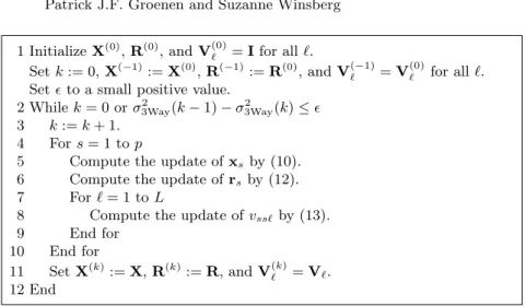
The3WaySym-Scalalgorithm for minimizingσ2
3Way(X,R,V1, . . . ,VL)
1 InitializeX(0),R(0), andV(0) ` =Ifor all`. Setk:= 0,X(−1):=X(0),R(−1):=R(0), andV(−1) ` =V (0) ` for all`. Set²to a small positive value.
2 Whilek= 0 orσ2
3Way(k−1)−σ23Way(k)≤² 3 k:=k+ 1.
4 Fors= 1 top
5 Compute the update ofxsby (10). 6 Compute the update ofrs by (12). 7 For`= 1 toL
8 Compute the update ofvss`by (13).
9 End for
10 End for
11 SetX(k):=X,R(k):=R, andV(k)
` =V`.
12 End
Fig. 2.The3WaySym-Scalalgorithm.
Instead of reportingσ2
3Way, we shall reportσ3Way2 /η2 with
η2=X ` X i<j wij([δij`(U)]2+ [δ(L)ij`]2) because σ2
3Way/η2 will be between 0 and 1 at a local minimum and is
in-dependent of the number of objects, the size of the dissimilarities, or the weights.
4
Synthesized Musical Instruments
To illustrate our method, we consider an empirical data set where the entries in each of two dissimilarity matrices are an interval of values. These two dissimilarity matrices represent dissimilarities among the same set of objects, given by the same expert on two different occasions; thus combined these two dissimilarity matrices to form a three-way two-mode array. The objects in the study are ten sounds differing with respect to only two physical parameters: the spectral center of gravity and the log attack time. Many previous studies of musical timbre have demonstrated that these two physical parameters are highly correlated with the perceptual axes uncovered when dissimilarity judgments are collected for sounds from different musical instruments playing the same note with the same loudness for the same duration of time.
Until some 35 years ago timbre was considered to be a perceptual param-eter of sound that was complex and multidimensional, defined primarily by what it was not, that is what distinguishes two sounds presented in the same manner equal in pitch, subjective duration and loudness (see Plomp, 1970). MDS studies have shown that these two attributes of sound, namely spectral
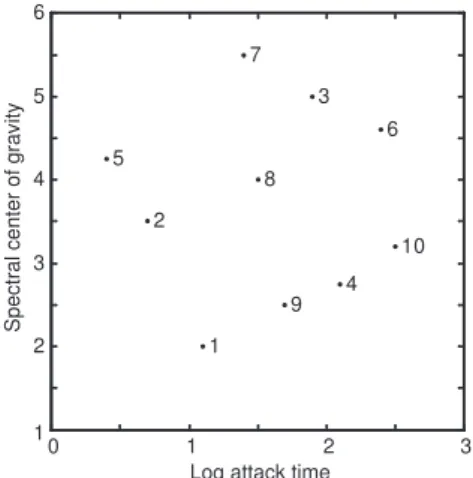
center of gravity and log attack time explain the factors we use to distinguish, say, middle C on the piano from middle C on some other instrument when they are played at the same loudness and the same duration of time (see, for example, McAdams, Winsberg, Donnadieu, DeSoete & Krimphoff, 1995; McAdams & Winsberg, 1999). So, when middle C is played on the piano the sound has some unidimensional attributes such as pitch, corresponding to the fequency of the fundamental, loudness, and duration. In addition, it is characterized by its timbre, that is, a note played by a piano and not some other musical instrument. This last attribute, timbre, is perceptually multidi-mensional with two important underlying perceptual dimensions relating to spectral center of gravity and log attack time. The spectral center of gravity is the weighted average of the harmonics generated when a note is sounded averaged over the duration of the tone with a running time window of, say, 12ms, and is higher for the harpsichord than for the piano, for example. The log attack time is the logarithm of the rise time measured from the time the amplitude envelope reaches a threshold of 2% of the maximum amplitude to the time it takes to reach the maximum amplitude, and is longer for a wind instrument like the trumpet than for a string instrument like the harp. The ten sounds in this study were generated artificially to represent the range of values found in natural instruments according to the design in Figure 3. The data represents dissimilarity judgments from the same expert listener taken on two occasions. The data are given in Table 2 of Groenen et al. (2006). On each occasion the expert listened to each pair of sounds and indicated a range of dissimilarity for each pair on a calibrated slider scale going from very similar to very different.
0 1 2 3 1 2 3 4 5 6 1 2 3 4 5 6 7 8 9 10
Log attack time
Spectral center of gravity
Fig. 3. Design of the ten sounds according to spectral center of gravity (vertical axis) and log attack time (horizontal axes).
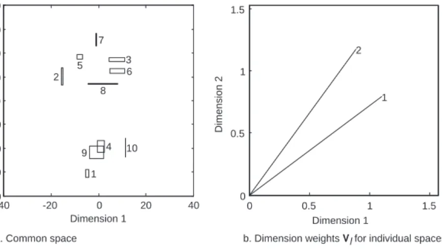
The data were analyzed by 3WaySym-Scal for both occasions simul-taneously. To reduce the probability of a bad local minimum we have used 100 random starts and chose the best one. The resulting solution with Stress 0.05194421 is shown in Figure 4. Here, the common space withX andR is shown in the left panel. The right panel shows the weights for the two oc-casions. We see that at Occasion 1, the first dimension is emphasized more than the second, whereas this situation is reversed at Occasion 2. Another representation of this very same solution can be obtained by showing the individual spaces for each of the occasions, thus using theXV1 andRV1 for
the first occasion andXV2andRV2 for the second occasion. This
represen-tion of the individual spaces is shown in Figure 5. We also present the results obtained analyzing the data from occasion one and occasion two separately using theI-Scalalgorithm that is two separate two-way analyses in Figure 6. -40 -20 0 20 40 -40 -30 -20 -10 0 10 20 30 40 1 2 3 4 5 6 7 8 9 10 Dimension 1 Di m en sion 2 0 0.5 1 1.5 0 0.5 1 1.5 Dimension 1 Dim en sion 2 1 2
a. Common space b. Dimension weights Vl for individual spaces
Fig. 4.Common space and dimension weights for the3WaySym-Scalsolution for judgements on synthesized musical instruments for judgements on two occasions by a single professional judge.
It is informative to examine and compare the three-way solution treating the two data matrices simultaneously obtained with 3WaySym-Scal with the solutions obtained for each occasion separately using the two-wayI-Scal algorithm. In each case, the horizontal axis represents log attack time and the vertical axes the spectral center of gravity. Without imposing any restric-tions, each version of SymScal seems to be able to reconstruct the physical space. The results for the 3WaySym-Scal in Figure 4 indeed reflect the physical space. Notice the groupings 10, 9, 4, 1 and 2, 5, 7 and 3, 6, 8 reflect how these stimuli are grouped in the physical space. Moreover, the relation of these groups to one another approximates their disposition in the physical space reasonably well. The results for the second occasion analyzed alone
a. Occasion 1 b. Occasion 2 -40 -20 0 20 40 -40 -30 -20 -10 0 10 20 30 40 1 2 3 4 5 6 7 8 9 10 Dimension 1 D im ension2 -40 -20 0 20 40 -40 -30 -20 -10 0 10 20 30 40 1 2 3 4 5 6 7 8 9 10 Dimension 1 Di m en sion 2
Fig. 5. Three-way interval MDS solution for judgements on synthesized musical instruments for judgements on two occasions by a single professional judge.
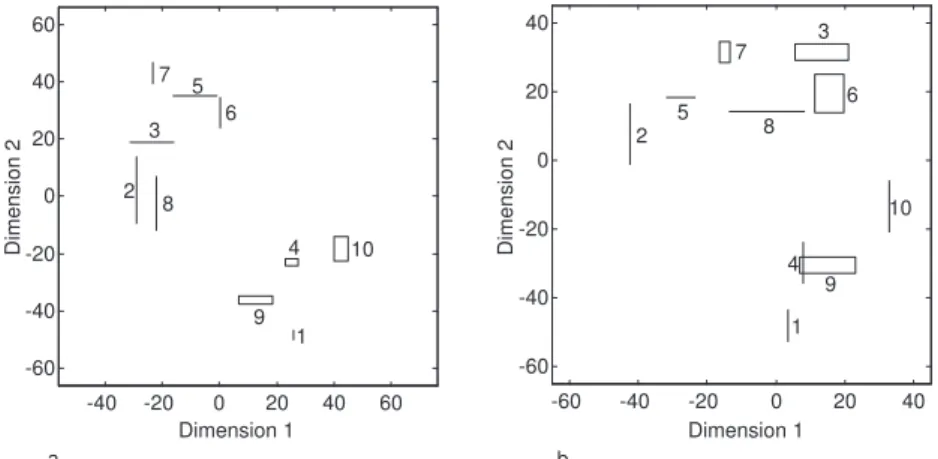
-40 -20 0 20 40 60 -60 -40 -20 0 20 40 60 -60 -40 -20 0 20 40 -60 -40 -20 0 20 40 Dimension 1 Dimension 1 b. a. Dimension 2 Dimension 2 1 2 3 4 5 6 7 8 9 10 1 2 3 4 5 6 7 8 9 10
Fig. 6.UnconstrainedI-Scalsolutions for the sound data obtained by Groenen et al. (2006). Panel (a) gives the results for Occasion 1 with I-Stress .02861128 and Panel (b) for Occasion 2 with I-Stress .04893295.
reflect the physical space the best, and the solution from the first occasion alone shows the most deviations from the physical space: 8, 3, 6 are too far to the left, 3 is too low, 7 is too far to the left, and 1 is too far to the right. Note that these differences from one occasion to another are greater than the range of uncertainty reflected in the solutions. Analyzed alone without look-ing at the three-way solution one might want to conclude that the improved results on the second occasion indicate that the task is better performed with some practice and with greater familiarity with the group of sounds. How-ever, the expert spent much time familiarizing himself with the sounds before undertaking the task. The results of the three-way analysis combined with
the two-way solutions point to the much more interesting idea that greater attention to the spectral center of gravity was necessary to better reproduce the physical space. This additional most interesting information about sound perception could only be teased out by examining all the results. Of course, it also appears from the figures that sounds with long attack times are more difficult to localize, than those with short attack times (with exception to sound number 10).
5
Discussion and Conclusions
We have presented an MDS technique for symbolic data that deals with three-way two-mode fuzzy dissimilarities consisting of a interval of values observed for each pair of objects, for each source. In this technique, each object is rep-resented as a series of hyperboxes in apdimensional space. By representing the objects as hypercubes, we are able to convey information contained when the dissimilarity between the objects or for any object pair needs to be ex-pressed as a interval of values not a single value, and when one has data from more than one source. It may be so, moreover, that the precision inherent in the dissimilarities is such that the precision in one recovered dimension is worse than that for the other dimensions. Our technique is able to tease out and highlight this kind of information.
The 3WaySym-Scal algorithm for MDS of interval dissimilarities is based on iterative majorization, and the I-Scal algorithm created to deal with the case when dissimilarities are two-way, one-mode data and are given by a range or interval of values. The advantage is that each iteration yields better 3Way-IStress until no improvement is possible. Simulation studies have shown thatI-ScalandHist-Scalupon which this algorithm is based, com-bined with multiple random start and a rational start yields good quality solutions.
Denœux and Masson (2000) discuss an extension for interval data that allows the upper and lower bounds to be transformed. Although it is techni-cally feasible to do so in our case, we do not believe that transformations are useful for symbolic MDS with interval or histogram data. The reason is that by having the available information of a given interval for each dissimilarity, it seems unnatural to destroy this information. Therefore, we recommend applying symbolic MDS without any transformation.
The present model can be extended along at least two lines. First, one could allow for individual rotations of the common space. It remains to be studied how this could be implemented. For example, one could only rotate
Xand notRor one could do both. A second line of extensions could study the use of intervals forV`as well. The consequences also rquire further study.
References
BORG, I. and GROENEN, P.J.F. (2005):Modern Multidimensional Scaling: Theory
and Applicatons, Second Edition Springer, New York.
CARROLL, J.D. and CHANG, J.J. (1972): Analysis of individual differences in multidimensinal scaling via an N-way generalization of Eckart-Young decom-position.Psyhometika, 35, 283-319.
DE LEEUW, J. and HEISER, W.J. (1980): Multidimensional scaling with restric-tions on the confguration. In P. R. Krishnaiah (Ed.), Multivariate analysis
(Vol. V)(pp. 501-522). Amsterdam, The Netherlands: North-Holland.
DENŒUX, T. and MASSON, M. (2000): Multidimensinal scaling of interval-valued dissimilarity data.Pattern Recognition Letters, 21, 83-92.
GROENEN, P.J.F., WINSBERG, S., RODRIGUEZ, O. and DIDAY, E. (2006): I-Scal: Multidimensionl scaling of interval dissimilarities.Computational Statis-tics and Data Analysis, 51, 360-378.
GROENEN, P.J.F., and WINSBERG, S. (2006): Multidimensional scaling of his-togram dissimilarities. In V. Batagelj, H.-H. Bock, A. Ferligoj, and A. Ziberna (Eds.), Proceedings of the ICFS Llubjana, Slovenia (pp. 161-170). Springer, Berlin.
KRUSKAL, J.B. (1964): Multidimensional scaling by optimizing goodnes of fit to a nonmetric hypothesis.Psychometrika, 29, 1-27.
MASSON, M. and DENŒUX, T. (2002): Multidimensional scaling of fuzzy dissim-ilarity data;Fuzzy Sets and Systems, 128, 339-352.
MCADAMS,S. and WINSBERG,S. [1999]: Multidimensional scaling of musical tim-bre constrained by physical parameters. The Journal of the Acoustical Society of America, 105, 1273.
MCADAMS,S., WINSBERG,S., DONNADIEU, S., DESOETE,G., and KRIM-PHOFF,J. (1995) Perceptual scaling of synthesized musical timbres: Common dimensions, specificities, and latent subject classes. Psychological Research, 58, 177-192.
PLOMP, R. (1970) : Timbre as a multidimensional attribute of complex tones. In R. Plomp & G.F. Smoorenburg (Eds.) Frequency analysis and periodicity
dectection in hearing (pp 397-414. Leiden: Sijthoff
WINSBERG, S. and CARROLL, J.D. (1989): A quasi-nonmetric method for mul-tidimenional scaling via an extended Euclidean model.Psychomtrika, 54, 217-229.
WINSBERG, S. and DESOETE, G. (1993): A latent class approach to fitting the weighted Euclidean model, CLASCAL.Psychometika, 58, 31-330.