Bayesian Near-Boundary Analysis in Basic
Macroeconomic Time Series Models
∗Michiel De Pooter1 Francesco Ravazzolo2 Rene Segers3 Herman K. Van Dijk3,† 1Federal Reserve Board
2Norges Bank
3Tinbergen Institute and Econometric Institute
Erasmus University Rotterdam
Econometric Institute Report EI 2008-13
August 21, 2008
Abstract
Several lessons learnt from a Bayesian analysis of basic macroeconomic time series models are presented for the situation where some model parameters have substantial posterior probability near the boundary of the parameter region. This feature refers to near-instability within dynamic models, to forecasting with near-random walk models and to clustering of several economic series in a small number of groups within a data panel. Two canonical models are used: a linear regression model with autocorrelation and a simple variance components model. Several well-known time series models like unit root and error correction models and further state space and panel data models are shown to be simple generalizations of these two canonical models for the purpose of posterior inference. A Bayesian model averaging procedure is presented in order to deal with models with substantial probability both near and at the boundary of the parameter region. Analytical, graphical and empirical results using U.S. macroeco-nomic data, in particular on GDP growth, are presented.
Keywords: Gibbs sampler, MCMC, autocorrelation, nonstationarity, reduced rank models, state space models, error correction models, random effects panel data models, Bayesian model averaging
JEL Classification Codes: C11, C15, C22, C23, C30 ∗This paper is a substantial revision and extension of De Pooter
et al.(2006). We are very grateful to participants of the 3rdWorld Conference on Computational Statistics & Data Analysis (Cyprus, 2005), the International Conference on Computing in Economics and Finance (Geneva, 2007), and the Advances in Econometrics Conference (Louisiana, 2007), for their helpful comments on earlier versions of the paper and we are in particular indebted to William Griffiths, Lennart Hoogerheide and Arnold Zellner for many useful comments. Herman Van Dijk gratefully acknowledges financial support from the Netherlands Organization for Scientific Research (NWO). The views expressed in this paper are solely the responsibility of the authors and should not be interpreted as reflecting the views of the Board of Governors of the Federal Reserve System or of any other employee of the Federal Reserve System nor the views of Norges Bank (the Central Bank of Norway).
This paper contains a number of references to Appendices. These appendices contain sampling schemes, conditional and marginal density results, probability density functions and an overview of models used in the paper. They are available on http://people.few.eur.nl/hkvandijk/research.htm. Also given on this website is the computer code and data which was used in the empirical applications in the paper.
†Corresponding author. Tinbergen Institute, Erasmus University Rotterdam, P.O. Box 1738, NL-3000 DR Rotterdam, The Netherlands. Tel.: +31-10-4088900, fax: +31-10-4089031. E-mail addresses:
[email protected] (M. De Pooter), [email protected] (F. Ravazzolo),
1
Introduction
Stable economic growth with possibly temporary periodic deviations - better known as business cycles - is one of the most important economic issues for any country. A widely used macroeconomic time series to measure these characteristics of growth and cycles is real Gross Domestic Product. A commonly used model in this context is the linear autoregressive model with deterministic trend terms. Using such time series and model classes, econometric analysis -Bayesian and Non-Bayesian- leads for most industrialized nations to substantial evidence that economic growth evolves according to a trend process that is largely determined by stochastic shocks. Otherwise stated, in the autoregressive models one finds substantial empirical evidence of a characteristic root that is near the boundary of unity or at this boundary in the parameter region. There exists an enormous literature on this topic; here we only mention the well-known study of Nelson and Plosser (1982) and for empirical evidence on industrialized nations over the past century we refer to Van Dijk (2004).
There are several other examples in macro economics of the existence of substantial posterior probability near the boundary of a parameter region. In business cycle analysis one may be interested to know how much of the variation in an economic time series is due to the cycle and how much is due to the trend. This issue is relevant in the context of an adequate policy mix for stimulating long term economic growth and short term business cycle control. Using a structural time series model one may find substantial posterior probability of the cyclical component near zero and the relative weights of the trend and cyclical components are then very uncertain. Another example occurs with typical characteristics of financial time series in stock markets. These series behave close to a random walk model or, otherwise stated, close to a model with a characteristic root close to the boundary of unity. The economic issue of such a process is whether financial markets are efficient in the sense that the optimal forecast for future stock market prices is the current price. A fourth example is the club or cluster behavior in panel data models for economic growth in industrialized nations. In this context, convergence of economic growth is studied and the number of clusters may be relatively small. Substantial probability may occur at the boundary of the parameter region of the number of clubs and, as a consequence, large uncertainty exists with respect to the correct number of clubs.
To explore the issue of Bayesian near-boundary analysis in basic economic time se-ries models, one derives their likelihoods and specifies prior information. Our approach with respect to specifying prior information is to start with uniform priors on a large region. The use of such noninformative priors means that we concentrate on the infor-mation content in and the shape of the likelihood function. Given our diffuse priors, the posterior distributions of parameters of interest may or may not exist. The latter occurs, in particular, at the boundary of the parameter region, due to nonidentifiability of some parameters of interest. We discuss how Information matrix priors or training sample priors may regularize or smooth the shape of irregular posterior distributions. In our analysis we make use of an interplay of analytical techniques, simulation methods and graphics. As a simulation technique we use the Gibbs sampling method. A brief introduction is given in Section 2. We note that graphs in the context of Bayesian analysis are becoming more and more important see, for example, Murrell (2005). In our analysis we therefore also place emphasis on presenting results in a graphical way.
In this paper we make use of two classes of canonical models. The first class of models is known as the class of single equation dynamic regression models. A first contribution
of this paper is to show that, for our purpose of a Bayesian near-boundary analysis in the parameter region, basic members of this class of models like unit root models, distributed lag models and error correction models are special cases of the well-known linear regression model with first-order autocorrelation in the disturbances. We also indicate that an error correction model with near unit root behavior is - for posterior analysis - equivalent to an instrumental variable regression model with possibly weak instruments; see also Hooger-heide and Van Dijk (2001) and HoogerHooger-heide and Van Dijk (2008). Interpretation of the models, their posteriors and the effect of smoothness priors like the Information matrix and training sample priors is one aim. A second aim is to illustrate a Bayesian analysis of economic growth in U.S. Gross Domestic Product using different model specifications.
The second class of models deals with variance parameters as parameters of interest. We discuss how the simple regression model with heteroscedasticity can be used as an introduction to the class of Hierarchical Linear Mixed Models (HLMM). As a second contribution, we show that the latter model serves as a parent class for time-varying parameter models such as state space models and panel data models. We investigate what happens when the density of one of the variance parameters is located near the zero bound and what happens when the number of components/groups in a panel is very small. We show that the latter case also leads to a boundary issue. We note that a combination of the first and second class of basic models has recently become important in empirical analysis.
A third contribution of this paper is to show how Bayesian model averaging over models with substantial posterior probability near and at the boundary leads to better forecasting. That is to say, we do not consider the case where substantial posterior probability is near and/or at the boundary as an econometric inferential problem where model selection is appropriate in order to determine or test whether the economic process is stationary or nonstationary but as a case where model averaging is to be preferred. This may lead to improved forecasting.
The results of our analysis may be summarized as ‘lessons learnt from models used’ and the start of a road map for learning Bayesian near-boundary analysis. A summary is presented in Section 7. Some key lessons are: investigate the shape of the likelihood of the parameters of interest; investigate the influence of smoothness priors in case of substantial near-boundary posterior probability; learn which simulation technique may be used efficiently in which situation; apply Bayesian model averaging over models with posterior probability near a boundary and models with substantial probability at the boundary. The topic of this paper should be of interest to Bayesians who make use of basic regression models for economic time series when the focus is on the information content of the likelihood. The topic should interest non-Bayesians who are very knowledgeable about basic econometric models and want to learn how the information in the likelihood function of such models is summarized according to Bayes’ rule.
There exists an excellent literature of Bayesian analysis of regression models with auto-correlation, unit root models, distributed lag models, unobserved component models and panel data models. An incomplete list of references is given as Chib (1991), Chib and Greenberg (1994, 1995) and Chib and Carlin (1999), Schotman and Van Dijk (1991a,b) and Harvey (1989). The purpose of the present paper is to extend this analysis to situa-tions where substantial posterior probability is near or at the boundary of the parameter region. We emphasize that this paper does not result and is not intended to result in a simple message with respect to using one model, one particular prior and one simulation techniques. We do not believe in such simplistic claims but rather in a situation where
different priors, different models and simulation algorithms are suitable depending on the problem studied, the data, and the shape of the posterior of the model considered. Our purpose is to investigate a set of models and, next, to explore Bayesian model averaging.
The content of this paper is structured as follows. In Section 2 we briefly review some (artificial) examples of shapes of posterior densities that the researcher may encounter in econometric practice. We also give an introduction to Gibbs sampling. This method is very natural given our derivations of joint, conditional and marginal posteriors for the linear regression model and this model with possibly autocorrelated disturbances. In Section 3 we present some basic results for the linear regression model that will be used in subsequent sections. In Sections 4 and 5 we present our empirical analysis and present some theoretical results of near-boundary posterior probability for a number of models for economic time series. Section 6 deals with forecasting U.S. Gross Domestic Product (GDP) using Bayesian model averaging. Section 7 contains a summary of models used and lessons learnt. The Appendices contain some technical details. We note that the technical level of the paper is like that of an introductory graduate econometrics course. Matrix notation is used in order to indicate the common, linear (sub-)structure of several models.
2
Preliminaries I: Basics of Gibbs Sampling and Typical
Shapes of Posterior Densities
2.1 Basics of Gibbs sampling
As discussed in, for instance, Van Dijk (1999) and Hamilton (2006), the ‘simulation revolu-tion in Bayesian econometric inference’ is to a large extent due to the advent of computers with ever-increasing computational power. This allows researchers to apply alternative Bayesian simulation techniques for estimation in which extensive use is made of pseudo-random number generators. One of the most important and widely used simulation meth-ods is Gibbs sampling, developed by Geman and Geman (1984), Tanner and Wong (1987) and Gelfand and Smith (1990). This method has become a popular tool in economet-rics for analyzing a wide variety of problems; see for instance Chib and Greenberg (1996) and Geweke (1999). Judging from numerous recent articles in the literature, Gibbs sam-pling is still gaining more and more momentum. Recent textbooks such as Bauwenset al.
(1999), Koop (2003), Lancaster (2004), and Geweke (2005) discuss how Gibbs sampling is used in a wide range of econometric models, in particular in models with latent variables. Mixture processes are an important class of latent variable models in econometrics; the most well-known due to Hamilton (1989). In recent papers by, for instance, Celeux et al.
(2000), Fr¨uhwirth-Schnatter (2001), Jasra et al. (2005) and Geweke (2007), the issue of convergence of the Gibbs sampler in this class of models is discussed. The posterior dis-tribution in mixture processes may be multimodal and may exhibit ridges often due to near nonidentification of parameters. A detailed analysis of this topic is beyond the scope of the present paper but we note and will make use of the distinction by Geweke (2007) between the interpretation of a model and its posterior densities on the one hand and the numerical efficiency and convergence of a simulation algorithm on the other hand.
One may characterize the Gibbs sampling algorithm as an application of the divide-and-conquer principle1. First, a K-dimensional parameter vector θ is divided into m
1We are necessarily brief in our explanation of the Gibbs sampler. See e.g. Casella and George (1992), or Hoogerheideet al.(2008), for a more elaborate discussion.
componentsθ1, θ2, ..., θm, where m ≤K. Second, for many posterior distributions which
are intractable in terms of simulation the lower-dimensionalconditional distributions turn out to be remarkably simple and tractable. The Gibbs sampler exploits this feature, as it samples precisely from these conditional distributions. Its usefulness is, for example, demonstrated by Chib and Greenberg (1996) and Smith and Roberts (1993).
Since Gibbs sampling is based on the characterization of the joint posterior distribution by means of the complete set of conditional distributions, it follows that a requirement for application of the Gibbs sampler is that the conditional distributions, described by the densities
p(θi|θ−i), fori= 1, ..., m (1)
whereθ−i denotes the parameter component vector θ without theith component, can all
be sampled from. The Gibbs sampling algorithm starts with the specification of an initial set of values: (θ1(0), ..., θm(0)) and then generates a sequence
(θ(1)1 , ..., θ(1)m ),(θ (2)
1 , ..., θm(2)), ...,(θ (J)
1 , ..., θ(mJ)) (2)
following a process such that θ(ij) is obtained from p(θi|θ(−ji−1)). Thus, θ (j)
i is obtained
conditional on the most recent values of the other components. We may summarize the Gibbs sampling algorithm as follows:
1: Specify starting valuesθ(0)= (θ(0)1 , . . . , θm(0))
and setj= 1. 2: Generate (the jth Gibbs step) : θ1(j) fromp(θ1|θ(2j−1), . . . , θm(j−1)) θ2(j) fromp(θ2|θ(1j), θ (j−1) 3 , . . . , θ (j−1) m ) θ3(j) fromp(θ3|θ(1j), θ (j) 2 , θ (j−1) 4 , . . . , θ (j−1) m ) .. . θm(j) fromp(θm|θ( j) 1 , . . . , θ (j) m−1)
3: Ifj < J, set j=j+ 1, and go back to Step2.
The above algorithm yields a sequence of J realizations θ(j) = (θ1(j), ..., θ(mj)), for j =
1,2, ..., J, from a Markov chain, converging to the target distribution. We will refer to Step2 of the algorithm as ‘the Gibbs step’ and for each of the models that we discuss in the subsequent sections we will always indicate what the Gibbs step looks like. Note that the components ofθdo not necessarily need to be one-dimensional. Generating draws for blocks of parameters where some of theθi components denote a block of parameters is also
possible.
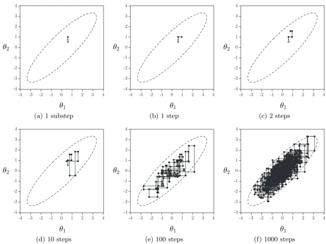
The Gibbs algorithm is illustrated in Figure 1 where we show an example path of Gibbs sampled points, when the conditional densities ofθ1|θ2andθ2|θ1are both standard Normal
and assuming a correlation coefficient of 0.75. The sample path is shown at different stages of the algorithm.
The key feature of Gibbs sampling is:
For large enough J the sequence of Gibbs draws, generated from the conditional distri-butions, is distributed according to the joint and marginal posterior distributions.2
Figure 1: Gibbs sampling: Example steps
(a) 1 substep (b) 1 step (c) 2 steps
(d) 10 steps (e) 100 steps (f) 1000 steps
Notes: Panels (a) through (f) show consecutive steps of the Gibbs sampler using two conditional posterior densities,p(θ1|θ2) andp(θ2|θ1) which are both standard normal with a correlation coefficient of 0.75. The open circles in Panels (a)-(f) indicate the starting vector (θ1(0), θ2(0)).
A simple argument for the general case is as follows. Supposeθi and θ−i have ajoint
posterior distribution with densityp(θi,θ−i). Thus this posterior should exist, which must
be carefully verified, compare also Sections 3 and 4. Then θ−i has themarginal posterior
distribution with density p(θ−i). Denote by θ−i and θj−1 the drawing generated in the
(j−1)thstep from the marginal posterior with densityp(θ−i). In the jth step of the Gibbs
sampling algorithm,θ(ij)is drawn fromp(θi|θ(−ji−1)), which is the density of the conditional
distribution of θi given θ(−ji−1). The joint density of θ (j) i and θ
(j−1) −i is
p(θi(j)|θ(−ji−1))p(θ−(j−1)i ) =p(θ(ij),θ(−j−1)i ). (3)
2Strictly speaking, sensitivity to initial conditions persists, but it becomes negligible if the sequence of Gibbs draws mixes sufficiently well.
Therefore, (θi(j),θ(−ji−1)) is distributed according to the joint posterior distribution. So the posterior is an invariant distribution of the Gibbs Markov chain, which is the invariant limiting distribution under the standard assumption of ergodicity. For a more detailed analysis on theoretical properties of the Gibbs sampler we refer to Smith and Roberts (1993), Tierney (1994) and Geweke (1999).
Because in practice it may take some time for the Markov chain to converge, it is common to discard the firstB draws, where typically B << J. These draws are referred to as the burn-in draws. Consequently, posterior results will be based only on draws
θ(B+1), . . . ,θ(J) of the generated chain. Furthermore, the sequence of draws sometimes displays some degree of autocorrelation. When autocorrelations are significant up to the (h−1)th lag, one can consider using only every hth draw and to discard the intermediate
draws (h is known as the thinning value)3. An altogether different approach is to generate
multiple Markov chains instead of just one chain and to use only the final draw from each sequence. Doing so implies that the Gibbs algorithm has to be executed a substantial number of times. When opting for this approach the researcher does not have to worry about which value to choose for h. Although the drawback of this method is that it can be very computationally intensive, it can alternatively help prevent posterior results from being (partially) determined by a particular set of starting values. We show in the next section that randomizing overθ(0) can be a worthwhile endeavor when the likelihood displays signs of multimodality.
2.2 Three typical shapes of posterior densities
To illustrate the kinds of shapes that may occur in posterior densities we work through a number of examples which are based on the model in Gelman and Meng (1991). Suppose that we have a joint posterior density of (θ1, θ2), which has the following form
p(θ1, θ2)∝exp
−12 aθ21θ22+θ21+θ22−2bθ1θ2−2c1θ1−2c2θ2
(4) where a, b, c1 and c2 are constants under the restrictions that a ≥ 0 and if a = 0 then
|b| <1 4. This Gelman and Meng (1991) class of bivariate distributions has the feature
that the random variables θ1 and θ2 are conditionally Normally distributed. In fact, the
conditional densitiesp(θ1|θ2) and p(θ2|θ1) can be derived (picked) directly from the right
hand side of (4) and can be recognized as Normal densities: p(θ1|θ2, a, b, c1, c2)∼ N bθ2+c1 aθ22+ 1, 1 aθ22+ 1 (5) p(θ2|θ1, a, b, c1, c2)∼ N bθ1+c2 aθ12+ 1, 1 aθ21+ 1 (6) Note that, typically, the joint density of (θ1, θ2) is not Normal. By choosing different
parameter configurations fora, b, c1 andc2 we can construct joint posterior densities with
rather different shapes, while the conditional densities remain Normal. In the remainder of this section we consider three types of shapes and we apply the Gibbs sampler to each
3The current consensus in the literature, however, seems to be to always include the information of all draws, even when these are correlated.
4These restrictions are to insure that the joint density in (4) is integrable and therefore a proper probability density function.
of these. Although the shapes are all in a way artificial since they are not based directly on a model and data, doing so will give us some early insights into different shapes of (joint) posterior densities and boundary issues which we discuss in detail in the remainder of this paper.
For each of the examples below thejthGibbs step consists of sequentially drawing from
(5) and (6):
jth Gibbs step for the Gelman-Meng model:
- generate θ(1j)|θ(2j−1) from p(θ1|θ2, a, b, c1, c2)∼ N bθ (j−1) 2 +c1 a θ(j−1) 2 2 +1, 1 a θ(j−1) 2 2 +1 ! - generate θ(2j)|θ (j) 1 from p(θ2|θ1, a, b, c1, c2)∼ N bθ (j) 1 +c2 a θ(1j) 2 +1, 1 a θ(1j) 2 +1 ! (i) Bell-shape
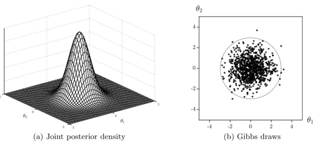
The first parameter configuration that we consider for the joint density in (4) is the fol-lowing; [a=b=c1 =c2 = 0] in which case the joint density is given by
p(θ1, θ2)∝exp−12(θ12+θ22)
(7) Both the conditional densities and the joint density are standard Normal. The latter is depicted in Figure 2(a). Gibbs sampling simply comes down to obtaining draws by iteratively drawing from standard Normal densities5. A scatterplot of one thousand of such draws is shown in Figure 2(b).
The estimated conditional means and variances are equal to 0 and 1 for both para-meters. These are exactly the parameters of the marginal densities which, in this case, we know to be standard Normal. In fact, for the chosen parameter configuration, the conditional and marginal densities coincide since the conditional density for θ1 does not
depend on θ2 and vice versa. In this particular example it would therefore obviously not
be necessary to use Gibbs sampling.
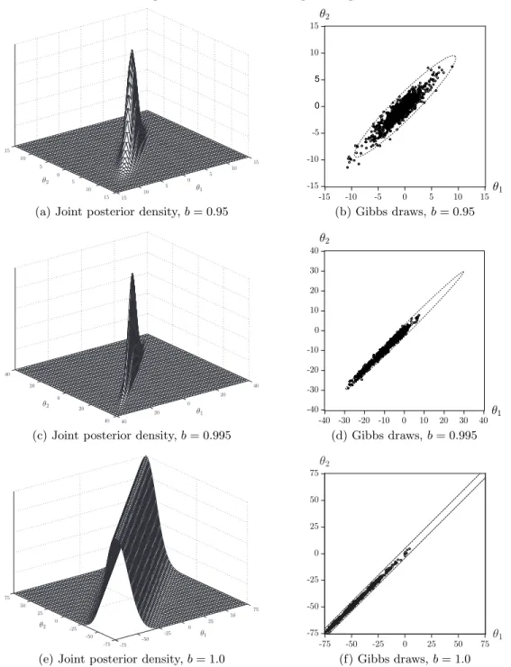
(ii) Ridges
The second parameter configuration that we examine is [a = c1 = c2 = 0]6. The joint
density is now given by
p(θ1, θ2) ∝ exp −12(θ 2 1−2bθ1θ2+θ22) (8) ∝ exp −12 θ1 θ2 1 b b 1 θ1 θ2
It is apparent from Figure 3 that the shape of this density depends on the value of b. When b tends to 1 a ridge along the line θ1 = θ2 appears in the shape of the posterior.
The scatterplots of Gibbs draws for this example in Figure 3 reveal that Gibbs sampling tends to become less efficient in such a case. Ridges may occur in econometric models where the Information matrix tends to become singular, that is whenb→1; see the next section for examples. We emphasize that the posterior in Figures 3(e) and 3(f) is defined on a bounded region with bounds -75 and +75. This posterior is constant along the diagonal and it is a continuous function defined on a bounded region and thus a proper density.
5For all three examples in this section we used a burn-in period ofB = 10,000 draws and we set the thinning valuehequal to 10.
Figure 2: Gelman-Meng: Bell-shape
(a) Joint posterior density (b) Gibbs draws
Notes: Panel (a) shows the Gelman-Meng joint posterior density forθ1 andθ2 given in (4) for parameter values [a = b = c1 = c2 = 0] whereas Panel (b) shows the scatterplot of 1,000 draws from the Gibbs sampler together with the 99% highest probability density region.
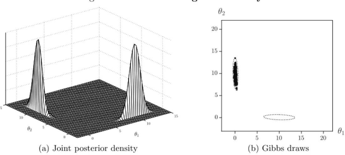
(iii) Bimodality
The third and final configuration we consider is [a= 1, b= 0] and large, but not necessarily equal, values forc1 and c2.7 Here we selectc1 =c2 = 10 which gives
p(θ1, θ2) ∝ exp −12[θ12θ22+θ12+θ22−20θ1−20θ2] (9) ∝ exp −12 θ1−10 θ2−10 1 0 0 1 θ1−10 θ2−10 +θ21θ22
At first sight the scatterplot of one thousand Gibbs draws, shown in Figure 4(b), seems perfectly reasonable and posterior means and variances can easily be computed. However, when inspecting the joint density as depicted in Figure 4(a) we immediately see that the joint density p(θ1, θ2) is bimodal and that the Gibbs sampler has sampled from one
mode but not from the other. Apparently it tends to get stuck in one of the two modes8. This is because the modes are too far apart with an insufficient amount of probability mass in between the two modes for the sampler to regularly jump from one to the other. Admittedly, substantially increasing the number of draws substantially will eventually lead to a switch. However, one cannot be certain when this will occur. The scatterplot shows that with a single run, one thousand draws is clearly not enough. However, although not shown here, also one million draws is still an insufficient number to witness a switch. Therefore, the Gibbs output only provides the researcher with information about a subset of the full domain ofp(θ1, θ2) and posterior results are thus incomplete. One option to try
and at least signal the bimodality of the likelihood is to execute the Gibbs sampler several times with widely dispersed initial values. However, we do note that even when doing so the issue of determining how much probability mass is located in each of the modes remains nontrivial. Although the example we discuss here is a rather extreme case, it
7See also Hoogerheideet al.(2007) for a further analysis of the three types of shapes (elliptical shapes, bimodality, ridges) for posterior densities in the IV model.
8Which of the two modes the Gibbs sampler gets stuck in depends on the initial values (θ(0) 1 , θ
(0) 2 ).
Figure 3: Gelman-Meng: Ridges
(a) Joint posterior density,b= 0.95 (b) Gibbs draws,b= 0.95
(c) Joint posterior density,b= 0.995 (d) Gibbs draws,b= 0.995
(e) Joint posterior density,b= 1.0 (f) Gibbs draws,b= 1.0
Notes: Panel (a) shows the Gelman-Meng joint posterior density forθ1 andθ2 given in (4) for parameter values [a =c1 =c2 = 0 andb = 0.95] whereas panel (b) shows the scatterplot of 1,000 draws from the Gibbs sampler together with the 99% highest probability density region. Panels (c) and (d) show the same figures forb= 0.995 and (e) and (f) forb= 1.0.
should be clear that multimodality can result in very slow converge for the Gibbs sampler. Multimodality may occur in reduced rank models when one is close to the boundary of the parameter region.
bimodal-Figure 4: Gelman-Meng: Bimodality
(a) Joint posterior density (b) Gibbs draws
Notes: Panel (a) shows the Gelman-Meng joint posterior density forθ1andθ2 given in (4) with parameter values [a = 1, b= 0 andc1 =c2 = 10] whereas panel (b) shows the scatterplot of 1,000 draws from the Gibbs sampler together with the 99% highest probability density region.
shaped density, indicate that it is essential to scrutinize a proposed model and the shape of its posterior distribution before moving on to drawing posterior inference on its parameters through a simulation method. Doing so may not always be straightforward, however, especially in large dimensional spaces.
3
Preliminaries II: Joint, Conditional and Marginal
Poste-rior and Predictive Densities for the Linear Regression
Model
3.1 Linear regression model
We start our model analysis by considering the basic linear regression model where the variation of a dependent variable yt is explained by a set of explanatory variables, as
summarized in the (1×K) (row-)vector xt where K is the number of variables in xt
(including a constant):
yt=xtβ+εt, t= 1, ..., T with εt∼i.i.dN(0, σε2) (10)
The goal is to draw inference on the (K×1) vector of regression parametersβ = (β1 β2. . . βK)′9
and the scalar variance parameter σ2
ε. In matrix notation, this model is given by
y=Xβ+ε with ε∼ N(0, σ2εIT) (11)
where y denotes the vector of T time-series observations or cross-sectional observations on the dependent variable, y = (y1 y2. . . yT)
′. X = (x′
1 x′2. . . x′T)′ denotes the matrix
of observations on the explanatory variables and IT is an identity matrix of dimension
(T ×T).
In the following we provide basic results for the joint, conditional and marginal posterior densities of the linear regression model in (11) which are useful for simulation purposes.
More details can be found in, e.g., Zellner (1971), Koop (2003) and Geweke (2005). For an expert reader we suggest to consider only the summary tables and diagrams in Appendix B.
Joint density
We start by specifying the likelihood for the linear regression model in (11) as: p(y|X, β, σ2ε) = (2πσ2ε)−T2 exp −21σ2 ε (y−Xβ)′(y−Xβ) (12) Combining the likelihood with a noninformative or Jeffreys’ prior10
p(β, σ2ε)∝(σε2)−1 (13)
gives the joint posterior density p(β, σε2|D)∝(σε2)− (T+2) 2 exp − 1 2σ2 ε (y−Xβ)′(y−Xβ) (14) where we defineD as the data information set, i.e. D≡(y, X).
A useful result to facilitate the derivation of the conditional and marginal posterior densities is to rewrite (14) by completing the squares onβ as
(y−Xβ)′(y−Xβ) = (y−Xβˆ)′(y−Xβˆ) + (β−βˆ)′X′X(β−βˆ) (15) with ˆβ = (X′X)−1X′y, the OLS estimator ofβ. One can now rewrite (14) as
p(β, σ2ε|D)∝(σ2ε)−(T+2)2 exp −21σ2 ε (y−Xβˆ)′(y−Xβˆ) + (β−βˆ)′X′X(β−βˆ) (16) The density (16) is known as the Normal Inverted-Gamma density of (β, σ2
ε), see Raiffa
and Schlaifer (1961, p. 310) and Zellner (1971, Chapter 3).
Conditional densities
The only part of the posterior in (16) which is relevant for determining the posterior density of β conditional on a value for σε2 is the part that depends on β. The first part,
(y−Xβˆ)′(y−Xβˆ), only depends on the dataDand does therefore not enter the conditional density ofβ. From the probability density functions given in Appendix C, we can recognize, for a given value ofσε2, a multivariate Normal density forβ which has mean vector M = ˆβ
and variance matrixS=σε2[X′X]−1, see equation (C-4). Similarly, the conditional density ofσ2
ε, for a given parameter vectorβ, follows from equation (C-3) and is Inverted Gamma 10A noninformative prior for the regression parameters can simply be specified as p(β) ∝ 1. For a variance parameter a noninformative prior comes down top(σ2)∝(σ2)−1 which follows from specifying a uniform prior for thelogarithm ofσ2, see Box and Tiao (1973), Chapter 1 for more details. If one has prior information it is strictly advisable to include this in the analysis (see the discussion in Lancaster, 2004 and Geweke, 2005). Specifying conjugate priors is, however, not always an easy task, especially when one is faced with a large dimensional parameter region. Here we focus on noninformative priors since we are concerned with what we can learn about the model parameters through the data likelihood.
with location parameter m = 12(y −Xβ)′(y −Xβ) and ν = 12T degrees of freedom. Summarizing, the conditional posterior densities are
p(β|D, σε2) ∼ Nβ, σˆ ε2[X′X]−1 (17) p(σ2ε|D, β) ∼ IG 1 2(y−Xβ) ′(y−Xβ),1 2T (18) Gibbs sampling for the basic linear regression model consists of iteratively drawing from the conditional densities p(β|D, σ2
ε) and p(σε2|D, β). A scheme of derivations for
Gibbs sampler results is presented in the top part of Figure 5. Thejth Gibbs step consists of
jth
Gibbs step for the linear regression model: - generate β(j)|σ2 ε (j−1) from p(β|D, σ2 ε)∼ N ˆ β, σ2 ε (j−1) [X′X]−1 - generate σ2 ε (j) |β(j) from p(σ2 ε|D, β)∼ IG 12(y−Xβ (j))′(y−Xβ(j)),1 2T Marginal densities
Ultimately, we are interested in learning about the properties of the marginal densities of βandσε2. In this model it is straightforward to derive these. Using the results of Appendix
C, the marginal posterior densities are given as
p(β|D) ∼ tβ,ˆ sˆ2[X′X]−1, T −K (19) p(σε2|D) ∼ IG 1 2(y−Xβˆ) ′(y−Xβˆ),1 2(T −K) (20) where ˆs2 = (y−Xβˆ)′(y−Xβˆ)/(T −K). A scheme for the derivations for the joint and marginal posterior densities of the linear regression model is given in Appendix B, Figure B-1. Since in this case one can directly simulate from the marginal densities without having to rely on the Gibbs sampler to obtain posterior results, we present direct sampling results in Appendix B, Figure B-2.
We emphasize that the derivation of conditional and marginal densities does not change if we were to replace xtβ by ρyt−1 in (10) using a uniform prior. That is, within a
noninformative Bayesian analysis one can go from a static analysis withxtβ to a dynamic
model: the posterior of regression parameters remains Student-t while in the frequentist world one cannot go from a static analysis to a simple dynamic analysis without a change in the properties of the OLS estimators. The same argument also hold for predictive densities which we discuss next.
Predictive densities
Suppose one is interested in constructing forecasts of future values of yt in the linear
regression model. A vector of Q future values, ye= [yT+1 yT+2 ... yT+Q]
′, is then assumed
to be generated by the following model:
e
y=Xβe +εe (21)
whereXe is aQ×K matrix of given values for the independent variables in the Qfuture periods andεeis aQ×1 vector of future errors which are assumed to be i.i.d. Normal with
zero mean and variance-covariance matrixσε2IQ. The marginal predictive density foreycan
be derived by integrating the joint densityp(ey, β, σ2
ε|X, De ) with respect toβ and σ2ε:
p(ye|X, De ) = Z σ2 ε Z β p(y, β, σe 2ε|X, De )dβ dσ2ε (22)
The joint density is specified as follows:
p(y, β, σe ε2|X, De ) =p(ey|β, σε2,Xe)p(β, σ2ε|D) (23) wherep(β, σ2
ε|D) is the posterior density in (14) and p(ye|β, σ2ε,Xe) is the conditional
pre-dictive density of ey in (21) which is given as: p(ye|β, σ2ε,Xe)∝(σ2ε)−12Qexp −2σ12 ε (ye−Xβe )′(ey−Xβe ) (24) which is a kernel of a multivariate Normal variable with meanXβe and covariance matrix σε2IQ. Scheme 1 shows a Gibbs sampling scheme for predictive analysis.
For each draw of (β, σ2
ε) one can draw ey from (24). The draws that are obtained in
this way are draws from the predictive density in (22). The joint density in (23) is a combination of (14) and (24) and becomes:
p(y, β, σe ε2|X, De )∝(σε2)−12(T+Q+2)exp h − 1 2σ2 ε (ye−Xβe )′(ye−Xβe )+(y−Xβ)′(y−Xβ)i (25) The first step toanalytically obtain the marginal predictive density follows from integrating with respect toσε2 which results in:
p(ey, β|X, De )∝[(ye−Xβe )′(ye−Xβe ) + (y−Xβ)′(y−Xβ)]−12(T+Q)
The second step is to complete the squares on β and to integrate with respect to the K elements ofβ which gives:
p(ey|X, De )∝[(T −K) + (ey−Xeβb)′H(ye−Xeβb)]−12(T+Q−K) (26)
where H = (I +Xe(X′X)−1Xe′)/sˆ2. Equation (26) indicates that ye has a multivariate Student-tdistribution with mean Xeβb, scale matrixH−1 and (T−K) degrees of freedom. By means of (26) one can draw directly from the predictive density. Schemes 2 and 3, both listed in Appendix B, summarize the derivations of distributions that are needed in a direct sampling and Gibbs sampling scheme.
We emphasize again that in a Bayesian noninformative framework all these derivations carry over directly to a dynamic model with lagged endogenous variables.
4
Single Equation Dynamic Regression Models
For this class of models the near-boundary issue refers to near-instability of dynamic mod-els. This is an important boundary issue in the sense that it has substantial implications for efficient forecasting. The purpose of this section is three-fold. We start with deriva-tions of posteriors of parameters of interest for different dynamic model specificaderiva-tions (and the construction of corresponding Gibbs samplers). We show here the uniformity of the
Figure 5: Sampling scheme: posterior and predictive results for Gibbs sampling
Posterior densities
prior density likelihood
p(β, σ2ε) L(β, σ2ε|D)
ց ւ
posterior density p(β, σε2|D)
ւ ց
conditional posterior ofβ conditional posterior ofσ2ε p(β|σε2, D)∼ Nβ, σb ε2(X′X)−1 p(σε2|β, D)∼ IG 1
2(y−Xβ)′(y−Xβ),12T
-Predictive densities
conditional posteriors ofβandσε2 p(β|σ2ε, D) p(σε2|β, D)
↓ (Normal - Inverted Gamma simulation)
conditional predictive density ofey p(ey|β, σ2
ε,X, De )∼ N(Xβ, σe ε2IQ)
↓ (Normal simulation)
marginal predictive density ofye
p(ye|X, De )
Notes: The figure presents results for Gibbs sampling schemes to obtain posterior and predictive results.
derivations for different model structures. We also discuss interpretation of the determinis-tic terms in autoregressive models with a focus on the issue of near-boundary analysis. The key feature in this context is: under what conditions do the dynamic economic processes under consideration return to a deterministic mean or trend and/or when does there exist a random walk or stochastic trend? Is there a substantial probability mass in the station-ary region and/or on the boundstation-ary of a random walk or stochastic trend model? These are boundary issues which have important implications for forecasting. Finally, we present empirical illustrations using some major U.S. macroeconomic and financial series.
4.1 Posterior analysis and Gibbs samplers
4.1.1 Linear regression with autocorrelation
We are now ready to analyze the extension of the model in (10) by allowing the error terms to have first-order autocorrelation11. That is:
yt = xtβ+νt, t= 1, ..., T (27)
νt = ρνt−1+εt, with εt∼i.i.dN(0, σ2ε) (28)
where ρ is the parameter that determines the strength of the autocorrelation. For ex-pository purposes with respect to the derivation of the conditional and marginal posterior densities we distinguish between two cases: one where the domain ofρis not restricted and one where it is. We emphasize that for economic purposes the domain of this parameter is in most cases restricted to the interval−1≤ρ≤1. We note that later we will distinguish between the cases whereρis 1 and whereρis in the bounded interval of (0,1). The domain for the remaining parameters is given by−∞< β <∞and 0< σ2
ε <∞. Whenρ= 0, the
autocorrelation model coincides with the basic linear regression model sinceνtreduces to a
white noise series. As we will see later, difficulties occur when there is a constant term and ρ has substantial posterior probability mass at the edges of its domain. By substituting (28) in (27) and rewriting the resulting expression in matrix notation, we obtain
y−ρy−1=Xβ−X−1βρ+ε, with ε∼i.i.dN(0, σ2εIT) (29)
where y−1 and X−1 denote the one-period lagged values of y and X. This reformulation
shows that the autocorrelation model is nonlinear in its parametersβ andρ. This problem of inference on a product (or ratio) of parameters is a classic issue. A detailed analysis is, however, beyond the scope of the present paper. For an early example see Press (1969) and we refer to Fieller (1954) and Van Dijk (2003) for more references. Although this issue of nonlinearity hampers parameter estimation and inference when using frequentist estimation approaches, obtaining posterior results using Gibbs sampling is straightforward as we will show below, in the case whereρ is unrestricted and no such deterministic terms as a constant or trend occur in the equation. We first turn to deriving the joint, conditional and marginal densities. It will become apparent that the autocorrelation model serves as a template for several other well-known econometric models.
Joint, posterior and marginal densities
The combination of the likelihood of the autocorrelation model with the noninformative prior in (13) and a uniform prior on ρ on a large region, and, further, assuming that the initial observations are fixed nonrandom quantities, gives the following joint posterior density, p(β, ρ, σ2ε|D)∝(σ2ε)−12(T+2)exp −21σ2 ε y−ρy−1−Xβ+X−1βρ ′ y−ρy−1−Xβ+X−1βρ (30) whereDonce again represents the known data (y, X). In case the domain of the parameter ρ is bounded, we make use of an indicator function I(β, ρ) which is 1 on the domain
11For a more general discussion on Bayesian inference in dynamic econometric models, we refer to Chib (1993) and Chib and Greenberg (1994).
specified (which is usually (−∞ < β < ∞),(−1 ≤ ρ ≤ 1) and 0 elsewhere). Thus, we obtain a truncated posterior density defined on the region indicated. We now derive the expression for the conditional densities p(β|ρ, σ2ε, D), p(ρ|β, σε2, D) and p(σ2ε|β, ρ, D) and
the marginal densitiesp(β|D) andp(ρ|D). For analytical convenience, we start with the derivations for the case whereρ is not restricted.
To facilitate the derivation of the conditional densities it is useful to rewrite the model in (29) in two different ways. In each case we condition on one of the two types of regression coefficients. First, we rewrite (29) conditional on values ofρ,
y∗=X∗β+ε where
y∗=y∗(ρ)≡y−ρy −1
X∗ =X∗(ρ)≡X−ρX−1 (31)
Second, we rewrite (29)conditional on values of β which then becomes ˜ y =ρy˜−1+ε where ˜ y= ˜y(β)≡y−Xβ ˜ y−1= ˜y−1(β)≡y−1−X−1β (32)
To derive the conditional density for β we use (31) to rewrite the joint posterior density. Doing so gives us the joint density of the basic linear regression model again so we can re-use all our earlier derivations. It therefore follows immediately that the conditional density forβ is multivariate Normal with mean m =βb∗ ≡(X∗′X∗)−1X∗′y∗ and variance matrix S = Sβ ≡ σ2ε(X∗′X∗)−1. Similarly, using (32) we obtain the result that the conditional
density for the unrestricted parameterρ is Normal with meanm= ˆρ≡(˜y−1′y˜−1)−1y˜−1′y˜
and variance s2 =σ2ρ ≡ σε2(˜y−1′y˜−1)−1. The conditional density forσ2ε is again Inverted
Gamma with parameter m= 12ε′ε≡ 12 y−ρy−1−Xβ+X−1βρ
′
y−ρy−1−Xβ+X−1βρ
and ν= 12T degrees of freedom. Summarizing, we have p(β|ρ, σ2ε, D) ∼ Nβ, Sb β p(ρ|β, σ2ε, D) ∼ N ρ, σb 2ρ p(σε2|β, ρ, D) ∼ IG 1 2ε ′ε,1 2T
Whereas in the basic regression model Gibbs sampling was unnecessary because the marginal densities could be derived analytically, here we do not have analytical results and therefore we need Gibbs sampling. This is due to the fact that the marginal densities of β, ρ and σ2
ε are not a member of any known class of densities. We show this as follows.
After integrating outσε2 from the joint density we get
p(β, ρ|D)∝h y−ρy−1−Xβ+X−1βρ′ y−ρy−1−Xβ+X−1βρi −T2
(33) We can rewrite this joint density in two different ways
p(β, ρ|D) ∝ y˜′My−˜ 1y˜+ (ρ−ρˆ) ′y˜ −1′y˜−1(ρ−ρˆ) −T 2 (34) p(β, ρ|D) ∝ y∗′MX∗y∗+ (β−β∗)′X∗′X∗(β−β∗) −T 2 (35)
whereMy−˜ 1 andMX∗ are idempotent residual maker matrices of ˜y−1andX
∗respectively12.
12The general residual maker matrix is given asMA= I
Integrating outρ from (34) andβ from (35) gives the marginal densities p(β|D) ∝ h(y−Xβ)′My −1−X−1β(y−Xβ) i−T−1 2 (y−1−X−1β)′(y−1−X−1β) −1 2 (36) p(ρ|D) ∝ h(y−ρy−1)′MX−ρX−1(y−ρy−1) i−T−K 2 (X−ρX−1)′(X−ρX−1) −12 (37) In case the parameter ρ is restricted to the interval [−1,1] we proceed as follows. Equations (30), (34) and (35) are now changed with inclusion of the indicator function I(β, ρ). The right hand side of equation (36) now contains the function c(β) given as c(β) = Φ1−ˆσρ ρ −Φ−1−ˆσ ρ ρ
where Φ stands for the standard Normal distribution function. The conditional normal density of ρgiven β,σ2ε and Dis in this case a truncated normal
density and the right hand side of equation (37) is now changed with the inclusion of the indicator function I(ρ) which is defined as 1 on the interval [−1,1] and 0 elsewhere.
Both densities in (36) and (37) - and their truncated variants - do not belong to a known class of density functions which means that we need Gibbs sampling to obtain posterior results. Despite the fact that the marginal densities of β and ρ can not be de-termined analytically, applying the Gibbs sampler is, however, a straightforward exercise, conditional upon the fact that all variables in the data matrix X have some nontrivial data variability.
Fisher Information matrix
The Fisher Information matrix can provide information as to whether problems are likely to occur when ρ approaches the edges of its domain, in the sense that the joint poste-rior density becomes improper. The Fisher Information matrix is defined as minus the expectation of the matrix of second order derivatives of the log likelihood with respect to the parameter vector θ = (β, ρ, σε2), i.e. I =−E[
δ2lnL(θ|D)
δθδθ′ ]. For the linear model with
autocorrelation the Information matrix is given by13
I=−E δ2lnL δρ2 δ 2lnL δρδβ′ δ 2lnL δρδσ2 ε δ2lnL δβδρ δ2lnL δβδβ′ δ 2lnL δβδσ2 ε δ2lnL σ2 εδρ δ2lnL δσ2 εδβ′ δ2lnL δσ4 ε = T 1−ρ2 0 0 0 (X−ρX−1)′(X−ρX−1) σ2 ε 0 0 0 2Tσ4 ε (38)
The inverse of the Information matrix shows that even when|ρ|= 1 none of the variances ‘explode’. In the next sections we will see that this not always needs to be the case. More general, under the condition that all variables in X have some variability, there are no issues in terms of impropriety of the joint posterior density when ρ reaches the edges of its domain.
13We note here that we focus on long term expectations which implies that E[y] = E[y
−l] = Xβ for l > 0. In reality,T is finite and therefore (small) sample means should be considered. For expositional purposes, however, we focus solely on long term expectations; see Kleibergen and Van Dijk (1994) for a finite sample analysis.
Gibbs sampling for the unrestricted case of ρ jth
Gibbs step for the linear regression model with autocorrelation:
- generate β(j)|ρ(j−1), σ2 ε (j−1) from p(β|ρ, σ2ε, D)∼ N c β∗(j−1), S(j−1) β - generate ρ(j)|β(j), σ2 ε (j−1) from p(ρ|β, σ2ε, D)∼ Nρˆ(j), σ2 ρ (j−1) - generate σε2(j)|β(j), ρ(j) from p(σ2 ε|β, ρ, D)∼ IG 1 2ε(j) ′ ε(j),1 2T
We can see from the conditional densities given earlier that the Gibbs sampler has no dif-ficulties with the nonlinearities in the likelihood. This is due to the fact thatconditionally
on one regression parameter, the model for the other regression parameter is the basic linear regression model as shown in (31) and (32). In fact, the joint posterior density of ρ and any element of β, or the other way around, resembles the density shown in Figure 2(a). Therefore, the Gibbs sampler is a very convenient tool for drawing inference on the parameters in these types of models.
We distinguish between a Gibbs step when there is no truncation forρ(then all draws are accepted) and the case of a truncated domain forρ. In the latter case, a simple solution for the Gibbs step is to ignore drawings outside the bounded region (−1< ρ <1). A more efficient algorithm has been developed by Geweke (1991, 1996).
4.1.2 Distributed lag models: Koyck model
A further extension of the basic linear regression model is the univariate distributed lag model14. This model has proven to be one of the workhorses of econometric modelling practice since it offers the econometrician a straightforward tool to investigate the depen-dence of a variable on its own history or on the history of exogenous explanatory variables. Here we focus in particular on the well-known Koyck model which is popular in for example marketing econometrics to investigate the dynamic link between sales and advertising. The general distributed lag model has, in principle, an infinite number of parameters. Koyck (1954) proposed a model specification in which the lag parameters are a geometric series, governed by a single unknown parameter. The resulting model is known as the geometric distributed lag model or simply as the Koyck model. Below, we discuss the boundary issue that can occur in this model which results in a parameter (near) nonidentification issue.
The Koyck model is given by
yt = βwt+νt, t= 1, ..., T (39) wt = (1−ρ) ∞ X i=0 ρixt−i (40) νt = ρνt−1+εt, with εt∼i.i.dN(0, σ2ε) (41)
where we allow for first-order autocorrelation in the error term. It is assumed that 0 ≤ ρ≤1, −∞< β <∞ and 0< σ2
ε <∞. Note that the effect of lagged values of the (here
single) explanatory variablextis determined solely byρand that this parameter is assumed
to be equal to the first-order autocorrelation parameter. In marketing econometrics the parameterρ is usually referred to as the ‘retention’ parameter.
We assume that νt is serially correlated. One may also assume that νt is i.i.d. Then
the transformed model has an MA(1) error. Another closely related model that also gives a boundary problem is the so called partial adjustment model15. This model is given as
y∗t = βwt+νt (42)
yt−yt−1 = (1−ρ)(y∗t −yt−1) +εt (43)
whereyt is observed buty∗t unobserved.
For the Koyck model, substituting (41) in (39) gives a similar type of expression as we found for the linear model with autocorrelation. In particular, with matrix notation one obtains
y−ρy−1=β(w−ρw−1) +ε
Equation (40) puts additional structure on the term w−ρw−1. More specifically, it holds
thatw−ρw−1 = (1−ρ)x which gives
y=ρy−1+β(1−ρ)x+ε, with ε∼ N(0, σε2IT) (44)
The result in (44) shows that the Koyck model is nested in the autocorrelation model and that therefore all earlier derivations hold here as well. The main difference, however, is that contrary to the autocorrelation model, the specific structure that is placed on the exogenous variable will result in a boundary issue whenρ is near 1. We can understand why this is the case by realizing thatβ will be near nonidentification for values of ρclose to 1. This means thaty effectively becomes a random walk and that exogenous variables no longer have any influence on y. When ρ = 1, then β is not identified and the model reduces to a random walk. We will analyze the joint, conditional and marginal densities to give insights in the consequences of the nonidentification ofβ when applying the Gibbs sampler.
Joint, posterior and marginal densities
Derivations for the joint and conditional densities are very similar to before. Therefore we only report the joint and conditional densities for the case of the bounded domain of ρ. The joint density, after integrating outσ2ε, is specified as
p(β, ρ|D) ∝h y−ρy−1−β(1−ρ)x ′ y−ρy−1−β(1−ρ)x i−T 2 I(β, ρ)
where I(β, ρ) is an indicator function which is 1 on the region bounded by 0 ≤ ρ ≤
1,−∞< β <∞and 0 elsewhere. The conditional densities - given thatρ is an element of the interval (0,1) - are given as
p(β|ρ, σ2ε, D) ∼ N β∗, σ2β p(ρ|β, σ2ε, D) ∼ T N ρ, σb 2ρ p(σε2|β, ρ, D) ∼ IG 1 2ε ′ε,1 2T
where T N indicates a Truncated Normal density. The parameters in the conditional densities are specified as
β∗ = (x∗′x∗)−1x∗′y∗=(1−ρ)2x′x−1x′(y−ρy−1) (45) σ2β = σε2(x∗′x∗)−1=σ2ε(1−ρ)2x′x−1 (46) and ˆ ρ = (˜y−1′y˜−1)−1y˜−1′y˜= (y−1−βx)′(y−1−βx) −1 (y−1−βx)′(y−βx) (47) σ2ρ = σε2(˜y−1′y˜−1)−1=σ2ε (y−1−βx)′(y−1−βx)−1 (48) andε′ε= y−ρy−1−β(1−ρ)x ′ y−ρy−1−β(1−ρ)x
. The density for ρis truncated to the unit interval which is indicated by the density notation T N.
At first sight, it may seem straightforward to apply the Gibbs sampler to the Koyck model. However, upon closer inspection of the conditional density parameters it becomes clear that a problem can occur for values of ρ close to 1. Suppose that a value near 1 is drawn for ρ. The conditional variance of β given this draw will be close to infinity, see (46), which means that any large value is likely to be drawn forβ. If the next draw forβis indeed large then the conditional variance ofρgoes to zero, see (48). As a result the next draw for ρ is again going to be close to 1, see (47). This means that the Gibbs Markov chain will converge very slowly. Convergence is not achieved for the case ρ= 1 since this is an absorbing state of the Markov chain. The extent of this problem depends on how much probability mass there actually exists close toρ= 1 and at ρ= 1.
When ρ = 1, it follows directly from the joint posterior p(β, ρ|D) that p(β|ρ = 1, D) is constant. Thus when ρ = 1 the conditional density of β is uniform on the interval (−∞< β <∞) and as a consequence it is improper. The conditional density of ρ is just the value of the truncated normal in the pointρ= 1. The economic issue is that we cannot learn (draw inference) on the parameter whenρ= 1, which is basically very natural for a random walk model.
To understand the behavior of the Gibbs sampler further we examine the marginal densities in detail. Given 0< ρ <1, the marginal densities forβ andρ are as follows:
p(β|D) ∝ h(y−βx)′My −1−βx(y−βx) i−T−1 2 (y−1−βx)′(y−1−βx) −1 2 c(β) (49) p(ρ|D) ∝ h(y−ρy−1)′M(1−ρ)x(y−ρy−1) i−T−1 2 x′x−12(1−ρ)−1 (50)
where c(β) is similar as in the previous section but now such that ρ is defined on the bounded interval (0,1).
Focusing on the density for ρ, we can recognize it to be a Student-t type density, but with an additional factor (1−ρ)−1. It is exactly this factor that is causing the behavior of the Gibbs sampler. The reason is that the joint densityp(β, ρ|D) is improper atρ = 1 for−∞ < β <∞. Graphically, this means that the joint density has a ‘wall’, similar to the ridge that was depicted in Figure 3(e). The marginal density forρwill tend to infinity whenρ tends to 1.
To reiterate what we said before, the extent of the problem - given the specification of the model - depends on the data at hand. If the likelihood assigns virtually no probability mass to the region close toρ= 1 then the marginal forβwill be virtually indistinguishable from a Student-tdensity. Furthermore, the marginal density forρwill still tend to infinitely close to ρ= 1, but if this event happens to be far out in the tail of the distribution then
this should not pose a serious problem. We shall show an example of this data feature in the empirical analysis relating to U.S. inflation and growth of real GDP. If, on the other hand, substantial probability mass is nearρ= 1 then measures should be taken to prevent the Gibbs sampler from reaching that part of the domain ofρ or, alternatively, to try and regularize the likelihood. Choosing an appropriate prior density can do the trick.
Fisher Information matrix
Analyzing the Information matrix gives similar insights in the irregularity in the joint density close to and equal toρ = 1 and furthermore, it provides us with a direction for a possible solution to tackle this irregularity. The Information matrix follows directly from (38) by substituting inX−ρX−1= (1−ρ)x. Therefore I= T 1−ρ2 0 0 0 (1−ρσ)22x′x ε 0 0 0 T 2σ4 ε (51)
The Information matrix again shows that when ρ is close to 1, the variance of ρ is zero (the inverse of the first diagonal element) whereas the variance of β goes to infinity (the inverse of the second diagonal element). Whenρ= 1, then the determinant of Information matrix is zero.
Gibbs sampling when 0< ρ <1
The Gibbsjth step is given by jth
Gibbs step for the distributed lag model:
- generate β(j)|ρ(j−1), σ2ε (j−1) from p(β|y, x, ρ, σ2ε)∼ N β∗(j−1), σ2β(j−1) - generate ρ(j)|β(j), σ2ε (j−1) from p(ρ|y, x, β, σ2ε)∼ T N ˆ ρ(j), σ2ρ (j−1) - generate σ2 ε (j) |β(j), ρ(j) from p(σ2 ε|y, x, β, ρ)∼ IG 1 2ε( j)′ε(j),1 2T
Whenρ is 1 it follows that Gibbs sampling is inappropriate.
Potential solutions: truncation of parameter region, Information matrix prior or training sample prior
In order to apply the Gibbs sampler without serious converge problems something should be done about the irregularity in the joint density close toρ = 1. A number of potential solutions have been proposed in the literature to circumvent this problem, see e.g. Schot-man and Van Dijk (1991a) and Kleibergen and Van Dijk (1994, 1998). Here we only briefly touch upon the several options in order to just give a flavor of how to tackle the impropri-ety of the likelihood. One can distinguish three solution approaches: (i) truncation of the parameter space, (ii) regularization by choosing a prior that sufficiently smoothes out the posterior, (iii) use of a training sample to specify a weakly informative prior forβ.
In terms of applying the first solution, one can truncate the domain of ρ and check whether there is probability mass near 1. Imposing an upper bound can be achieved by selecting for example a local uniform prior. The goal would be to only allow draws for ρ that are at leastη away from 1 withη >0 to prevent a wall in the joint posterior density.
Choosing a specific value forη would necessarily be a subjective choice. However, once a value forη is agreed upon one can apply the Gibbs sampler. Alternatively, one can use a Metropolis-Hastings type step in which only draws that fall below 1−η are accepted. For an example of this method, see e.g. Geman and Reynolds (1992).
As for the second solution, one can try and regularize the likelihood in the neighborhood ofρ= 1 such that it becomes a proper density. This can be achieved by using a prior that is chosen in such the way that it eliminates the factor (1−ρ)−1. From the Information matrix in (51) we can construct the following Jeffreys’ type prior forβ givenρ and σ2
ε,16 p(β|ρ, σ2ε)∝ (1−ρ) 2 σ2 ε for 0< ρ <1 (52)
Deriving the joint and marginal densities with this prior will show that it eliminates the factor (1−ρ)−1 from the marginal density ofρ. What happens is that the marginal density forρ is now integrable everywhere except for ρ = 1 which in turn has a zero probability of occurring.
The third solution is an alternative way of regularizing the posterior density. One can use a training sample17 to specify a weakly informative prior for β. Schotman and Van Dijk (1991a) specify the following prior
p(β|ρ, σε2)∝ Ny0, σ 2 ε (1−ρ)2 for 0< ρ <1 (53)
wherey0 is the initial value of the time-series fory. The intuition behind this prior is that
asρapproaches 1 it becomes increasingly difficult to learn aboutβ from the data since the unconditional mean ofy, given as (1−ρ)β, does not exist forρ at 1. The prior is stronger for smaller values of ρ but approaches an uninformative prior for ρ → 1. It is derived from the unconditional distribution ofy0 under the assumption of normality. The effect of
this Normal prior on the joint posterior density is that it eliminates the pronounced wall feature in the joint density. We will see an example of this approach when we discuss the Unit Root model.
We conclude that for solutions (ii) and (iii) one has to - in most cases - replace the simple Gibbs procedures by other Monte Carlo integration methods. This is a topic outside the scope of the present paper. Further solutions, which we do not discuss here in the detail, are to reparameterize the model in such a way that the Gibbs sampler can be used without any problems for the reformulated model. However, one still has to translate the posterior results back to the original model. Without imposing some sort of prior, similar problems will still occur only now at a different stage in the analysis. For examples of reparametrization see for instance Gilks et al.(2000). Finally, modified versions of the Gibbs sampler such as the Collapsed Gibbs sampler (see Liu, 1994), where some parameters can be temporarily ignored when running the Gibbs sampler (in this caseρ) can be useful in this context as well. In the empirical application in Section 5 we only use the truncation prior approach.
16In general the Jeffreys’ Information matrix prior is proportional to the square root of the determinant of the Information matrix of the considered model. For our purposes, however, we use a somewhat stronger prior because we need (1−ρ)2 instead of (1−ρ)1 to regularize the likelihood. For more details and an advanced analysis on similar Jeffreys’ priors we refer to Kleibergen and Van Dijk (1994, 1998).
4.1.3 Autoregressive models and error correction models with deterministic components
We present the issue of near-boundary analysis in the context of an autoregressive model with deterministic components. The simplest example is a first-order autoregressive model with an additive constant, given as
yt=c+ρyt−1+εt (54)
This model can be respecified as an error correction model (ECM) around a constant mean using a restriction onc. We start with rewriting (54) as
yt=µ(1−ρ) +ρyt−1+εt (55)
where c is now restricted as c =µ(1−ρ). We can rewrite the latter equation as a mean reversion model, see Schotman and Van Dijk (1991a,b),
∆yt= (ρ−1)(yt−1−µ) +εt (56)
Here one can see the expected ‘return to the long-term unconditional mean (µ) of the series’ when 0 < ρ < 1. That is, when yt−1 is greater than µ and 0 < ρ < 1, then the
conditional expected change in yt, given previous observations, is negative while in the
opposite case the expected change in positive. Furthermore, whenρtends to 1 then in the ECM specification (55) one has a smooth transition from stationarity to a random walk model. In other words one approaches the boundary in a continuous way. On the contrary in equation (54) one has a transition from stationarity to a random walk with drift: one hits the boundary with a ‘jump’. The models are much farther apart then the ones in the ECM setup. Note that the constant termc in (54) does not have a direct interpretation in terms of being the mean of the process while in (55) the constant µ is the long term unconditional mean of the series given 0< ρ <1.
Similar as for the Koyck model, imposing this particular ECM structure introduces a boundary issue when there is substantial posterior probability near ρ = 1. In the ECM model foryt, the interpretation ofµdepends on whether the series yis stationary (ρ <1)
or whether it has a unit root (i.e. ρ= 1). In the latter case, the mean of y does not exist and µ is thus nonidentified. Therefore, even when y is a weakly stationary process, any value forµalong the real line is likely to be drawn in the Gibbs sampler whenρis sampled close to 1. This will not only make it very difficult to pinpoint the posterior mean of µ but it also causes the sequence of draws forρ to have difficulties moving away fromρ= 1. Of course, ρ close to 1 can be an indication that one should model first differences of y instead of y itself which will circumvent the entire issue altogether. However, for series such as interest rate levels there is no clear economic interpretation why these should be I(1) processes and one is left with dealing with the boundary issue nonetheless.
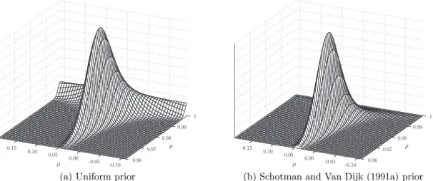
For series that are near unit root, substantial probability mass will lie close to ρ = 1 and at ρ = 1 so that the impropriety of the joint posterior poses a serious issue. As an example we depicted the joint density for the unit root model for a series of monthly data on the 10-year U.S. Treasury Bond yield in Figure 6(a). A time-series plot of this series is given in Figure 7(b). Figure 6(a) clearly shows the pronounced wall feature close to and at ρ = 1. In order to resolve the impropriety of the joint density a local uniform prior or truncation of the domain for ρ could be used. Another possibility would be to use a regularizing prior like the Schotman and Van Dijk (1991a) prior. The joint density that results from
Figure 6: Joint posterior density in the unit root model
(a) Uniform prior (b) Schotman and Van Dijk (1991a) prior
Notes: Panel (a) shows the joint posterior density p(ρ, µ|y) when we use a uniform prior as in (13) whereas panel (b) shows the same posterior density however now with the prior proposed by Schotman and Van Dijk (1991a) as given in (53). In both panels we use the end-of-month 10-year U.S. Treasury Bond constant maturity yield for the period January 1960-July 2007 as the data vectory.
combining the data likelihood with this particular prior is shown in Figure 6(b). The joint density no longer has a wall feature close toρ= 1 although it still flattens out somewhat near the edge of the domain. We note that this posterior may also be interpreted as the exact likelihood including the initial observation. For details see Schotman and Van Dijk (1991a).
We emphasize that the autoregressive model with an additive constant, equation (54), can be treated like the linear regression model of Section 3. Direct sampling or a simple Gibbs procedure is possible. The model with the ECM interpretation can be written as in the autoregressive form of Sections 4.1.1 and 4.1.2 and deriving the corresponding Gibbs sampling formulas is left to the interested reader. We also refer to that subsection for the convergence issues of the Gibbs sampler.
Next, we treat the autoregressive model with additive linear trend. We start with a distributed lag model of order two,
yt=c+βt+ρ1yt−1+ρ2yt−2+εt with εt∼i.i.dN(0, σ2ε) (57)
wheretcaptures a linear increasing trend. We can rewrite this model as an error correction model as follows. Consider
1−ρ1L−ρ2L2
(yt−µ−δt) =εt with εt∼i.i.dN(0, σε2) (58)
using c = µ(1−ρ1−ρ2) +δ(ρ1 + 2ρ2) and β = (1−ρ1 −ρ2)δ and where L is the lag
operator;Lyt=yt−1. Applying this operator to equation (58) we obtain
yt= (1−ρ1−ρ2)µ+δ(t−ρ1(t−1)−ρ2(t−2)) +ρ1yt−1+ρ2yt−2+εt (59)
This equation can be rewritten further as