DISSERTATION
submitted to the
Combined Faculty for the Natural Sciences and
Mathematics
of
Heidelberg University, Germany
for the degree of
Doctor of Natural Sciences
put forward by
M.Sc. Vera Trajkovska
born in Kumanovo
Learning Probabilistic Graphical Models
for
Image Segmentation
Advisors: Prof. Dr. Christoph Schnörr
Prof. Dr. Björn Ommer
Zusammenfassung
Probabilistische grafische Modelle bieten ein mächtiges Framework für die Darstellung von Strukturen in Bildern. Auf diesem Konzept basierend wurden viele Inferenz-und Lernalgorithmen entwickelt. Jedoch, sowohl Lernen als auch Inferenz sind im allgemeinen Fall kombinatorische NP-harte Probleme. Infolgedessen wurden Relax-ierungsmethoden entwickelt um die Originalprobleme zu approximieren aber mit dem Vorteil, dass sie vom Rechenaufwandt effizient sind. In dieser Arbeit betrachten wir das Lernproblem von binären graphischen Modellen und deren Relaxierungen. Zwei neuartige Methoden zum Bestimmen der Modellparameter von diskreten Energiefunk-tionen aus Trainingsdaten werden vorgeschlagen. Das Lernen der Modellparameter löst elegant das Problem, diese heuristisch zu bestimmen.
Motiviert durch gängige Lernmethoden, die auf die Minimierung des Trainings-fehlers oder einer Verlustfunktion aufbauen, entwickeln wir eine neue Lernmethode ähnlich zu structural SVM. Jedoch von dem Gesichtspunkt der Optimierung ist diese einfacher. Wir benennen diese Methode als linearisierten Ansatz (LA), da er auf linear abhängige Potentiale beschränkt ist. Die Linearität von LA ist entscheidend um eine feste konvexe Relaxierung zu erhalten, die den Einsatz von Standard-Inferenz-Lösern zum behandeln der Teilprobleme ermöglicht die beim Lösen des Gesamtproblems auftreten.
Allerdings wird diese Art von Lernmethoden fast nie die optimale Lösung liefern oder perfekte Performance auf der ganzen Trainingsmenge. Was würde also passieren, wenn das gelernte grafische Modell auf den ganzen Trainingsdaten die exakte Ground-Truth-Segmentierung wiedergeben würde? Würde das einen Vorteil für die Vorhersage versprechen?
Inspiriert von inverser Optimierung nutzen wir die inversen linearen Program-mierung um eine weitere Lernmethode zu entwickeln, bezeichnet als inversen linearen Programmierungsansatz (invLPA). Dieser Ansatz verbessert die trainierten graphis-chen Modelle weiter unter Verwendung der zuvor eingeführten Methoden und ist fähig die exakten Ground-Truth-Daten auf der Trainingsmenge vorherzusagen. Die empirischen Ergebnisse aus der Umsetzung von invLPA geben Antworten auf unsere zuvor gestellte Frage.
LA ist in der Lage gleichzeitig die unären und paarweisen Potentiale zu lernen während dies mit invLPA wegen der gewählten Repräsentierung nicht möglich ist. Auf der anderen Seite jedoch ist invLPA bezüglich der verwendeten Fittingmethode sehr flexibel, da die Potentiale nicht auf eine feste Gestalt beschränkt sind.
Auch wenn die korrigierten Potentiale mit invLPA immer zu Ground-Truth- Seg-mentierung der Trainingsdaten führen, kann invLPA nur Korrekturen der Vorder-grundsegmente vornehmen. Wegen der relaxierten Problemformulierung beeinflußt dies jedoch nicht das endgültige Ergebnis der Segmentierung. Vielmehr, solange
wir mit vorberechneten Modellparametern einer hinreichend guten Lernmethode initialisieren, wird diese Schwäche von invLPA das endgültige Vorhersageergebnis nicht signifikant beeinflussen.
Die Performance von unseren vorgeschlagenen Lernmethoden wird sowohl auf synthetischen als auch auf realen Datensätzen evaluiert. Wir zeigen das LA konkur-renzfähig ist im Vergleich zu anderen Lernmethoden, die Verlustfunktionen verwenden basierend auf Maximum a Posteriori Marginal (MPM) und Maximum Likelihood Estimation (MLE). Darüber hinaus veranschaulichen wir die Vorteile des Lernens mit Hilfe von inverser linearer Programmierung. In einem weiteren Experiment demon-strieren wir die Vielseitigkeit von unseren Lernansätzen indem wir LA anwenden zum Lernen von Bewegungssegmentierung in Videosequenzen und vergleichen dies gegenüber state-of-the-art Segmentierungsalgorithmen.
Abstract
Probabilistic graphical models provide a powerful framework for representing image structures. Based on this concept, many inference and learning algorithms have been developed. However, both algorithm classes are NP-hard combinatorial problems in the general case. As a consequence, relaxation methods were developed to approximate the original problems but with the benefit of being computationally efficient. In this work we consider the learning problem on binary graphical models and their relaxations. Two novel methods for determining the model parameters in discrete energy functions from training data are proposed. Learning the model parameters overcomes the problem of heuristically determining them.
Motivated by common learning methods which aim at minimizing the training error measured by a loss function we develop a new learning method similar in fashion to structured SVM. However, computationally more efficient. We term this method as linearized approach (LA) as it is restricted to linearly dependent potentials. The linearity of LA is crucial to come up with a tight convex relaxation, which allows to use off-the-shelf inference solvers to approach subproblems which emerge from solving the overall problem.
However, this type of learning methods almost never yield optimal solutions or perfect performance on the training data set. So what happens if the learned graphical model on the training data would lead to exact ground segmentation? Will this give a benefit when predicting?
Motivated by the idea of inverse optimization, we take advantage of inverse linear programming to develop a learning approach, referred to as inverse linear programming approach (invLPA). It further refines the graphical models trained, using the previously introduced methods and is capable to perfectly predict ground truth on training data. The empirical results from implementing invLPA give answers to our questions posed before.
LA is able to learn both unary and pairwise potentials jointly while with invLPA this is not possible due to the representation we use. On the other hand, invLPA does not rely on a certain form for the potentials and thus is flexible in the choice of the fitting method.
Although the corrected potentials with invLPA always result in ground truth segmentation of the training data, invLPA is able to find corrections on the foreground segments only. Due to the relaxed problem formulation this does not affect the final segmentation result. Moreover, as long as we initialize invLPA with model parameters of a learning method performing sufficiently well, this drawback of invLPA does not significantly affect the final prediction result.
The performance of the proposed learning methods is evaluated on both synthetic and real world datasets. We demonstrate that LA is competitive in comparison
to other parameter learning methods using loss functions based on Maximum a Posteriori Marginal (MPM) and Maximum Likelihood Estimation (MLE). Moreover, we illustrate the benefits of learning with inverse linear programming. In a further experiment we demonstrate the versatility of our learning methods by applying LA to learning motion segmentation in video sequences and comparing it to state-of-the-art segmentation algorithms.
Acknowledgments
I would like to thank many people without which this thesis would not have been possible.
First of all I am very grateful to my supervisor Professor Christoph Schnörr for giving me the opportunity to join the RTG at the Faculty of Mathematics and Computer Science. Under his supervision I was able to benefit from his guidance, support, help and understanding. I am very fortunate, that I had the oppprtunity to have him as a supervisor and all my knowledge during my PhD studies I owe to him.
I would like to thank a lot Stefania without whom as well a lot of this work would not have happened. And of course Bogdan who guided me at the beginning of my PhD work. Many many thanks to Florian, first of all for proofreading this thesis. And for all the discussions, all the help not only for my work but also for my bike repair etc. For letting me share the office with him (and Stefania) for some time and for standing the “warmth” in our office. I am very thankful to Arati and Eva for being my first friends in Heidelberg. Special thanks goes to Barbara for our lunches together, all the time spent together and for always being able to listen to my complaints and problems. Thanks to Evelyn for all the administrative help. I would like to thank Freddie for all the help and discussions. I am thankful to Fabian for helping me optimize my code, swimming together etc. I would also like to thank all my colleagues which were also part of my PhD years: Ecaterina, Artjom, Tabea, Andreas, Francesco, Mattia, Robert, Jan, Leonid, Lucas, Ruben, Fabrizio, Judit, Alexander.
And I would like to express my deepest gratitude to Matthias for all the love, help and support I had from him the last two years. Who always encouraged me and belived in me. Thank you as well for proofreading my thesis. And finally I would like to thank my whole family my father Chedomir, my mother Frosina, my sister Violeta and my brother Simon. Even far away I always had your love and support. And I would have never been where I am today if it would not have been you encouraging me in all my goals.
Funding by the Deutsche Forschungsgemeinschaft via the research training group 1653 Spatio / Temporal Graphical Models and Applications in Image Analysis is gratefully acknowledged.
List of Publications
Part of this thesis has been published at a conference.
V. Trajkovska, P. Swoboda, F. Åström, and S. Petra, Graphical Model Parame-ter Learning by Inverse Linear Programming, LNCS 10302, pp. 323–334, Springer, 2017
Contents
Zusammenfassung v Abstract vii Acknowledgments ix List of Publications xi 1. Introduction 11.1. Overview and Motivation . . . 1
1.2. Related Work . . . 3 1.3. Contribution . . . 4 1.4. Organization . . . 5 1.5. Notation . . . 6 2. Background 11 2.1. Graphical Models . . . 11
2.1.1. Graph Theory Used in Image Processing and Analysis . . . . 11
2.1.2. Probabilistic Graphical Models . . . 13
2.1.3. Directed Graphical Models: Bayesian Networks . . . 14
2.1.4. Undirected Graphical Models: Markov Random Fields (MRF) 14 2.2. Basic Concepts in Convex Analysis and Optimization . . . 16
2.2.1. Convex Sets . . . 16
2.2.2. Convex Functions . . . 17
2.2.3. Gradient Descent Method . . . 20
2.2.4. Subgradient Method . . . 22
2.2.5. Newton Method . . . 23
2.3. Exponential Families . . . 24
2.3.1. Basic Definitions and Notions of Exponential Families . . . . 24
2.3.2. Properties of the Space of Mean Parameters M. . . 27
2.3.3. Properties of the Forward Mapping ∇A . . . 27
2.3.4. Properties of the Inverse Mapping ∇A∗ . . . 28
2.3.5. Exponential Families for Discrete Graphical Models . . . 30
2.4. Inference . . . 31
2.4.1. Approximate MAP Inference . . . 33
2.4.2. Variational Formulation . . . 35
2.4.3. Image Labeling Problem . . . 36
2.4.4. Graph Cuts . . . 36
2.5. Learning . . . 42
2.5.1. Probabilistic Parameter Learning . . . 42
2.5.2. Loss Minimizing Parameter Learning . . . 45
2.6. Inverse Linear Programming . . . 46
3. Metric Learning for Segmentation 49 3.1. Introduction . . . 49
3.2. Mahalanobis Distance Metric Learning . . . 50
3.3. Representative Existing Approaches . . . 52
3.3.1. Mahalanobis Metric Learning for Clustering . . . 52
3.3.2. Large-Margin Nearest Neighbors (LMNN) Method . . . 53
3.3.3. Metric Learning as Eigenvalue Optimization . . . 54
3.3.4. Online Metric Learning . . . 57
3.4. Numerical Optimization Techniques . . . 59
3.4.1. Gradient Descent and Projected Gradient Descent . . . 59
3.4.2. Minimizing the Maximal Eigenvalue of a Symmetric Matrix . 60 3.4.3. Stochastic Gradient . . . 61
3.5. Proposed Approach . . . 62
3.5.1. Objective Functions . . . 62
3.5.2. Optimization . . . 66
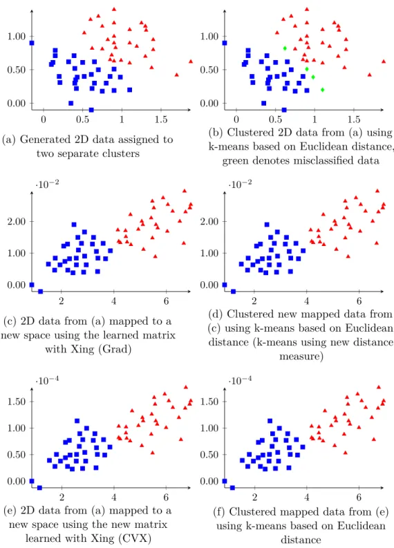
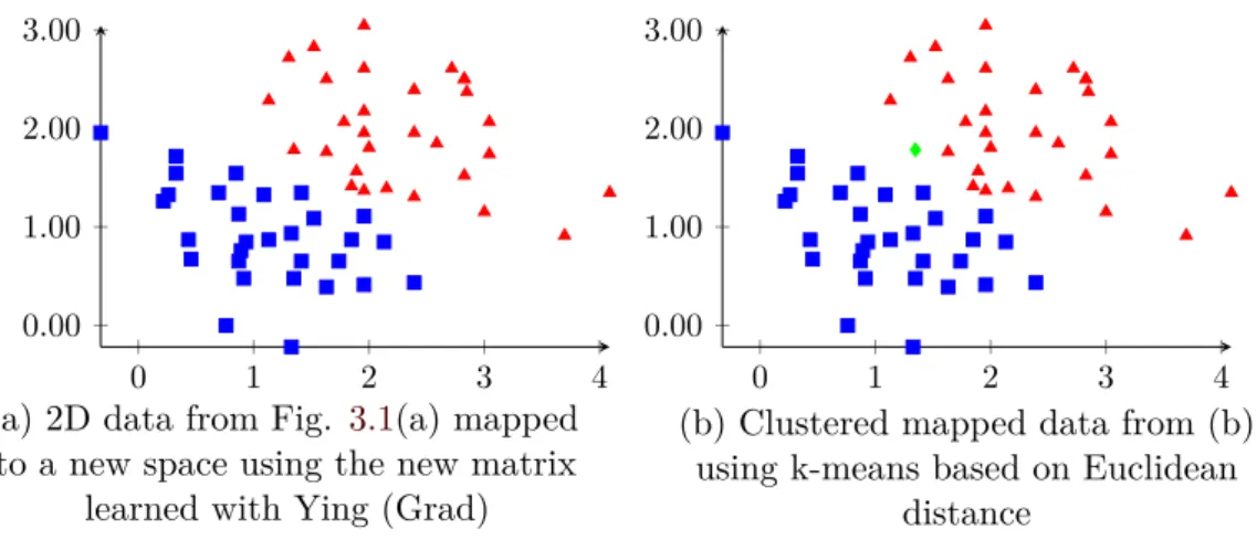
3.5.3. Experiments and Discussion . . . 71
4. Model Parameter Perturbation and Learning 77 4.1. Overview . . . 77
4.2. invLPA: Inverse Linear Programming Approach . . . 80
4.2.1. Model Parameter Perturbation . . . 80
4.2.2. Model Parameter Prediction . . . 83
4.3. LA: Linearly Parametrized Joint Learning Approach . . . 85
4.3.1. Model Parameter Perturbation . . . 85
4.3.2. Model Parameter Prediction . . . 87
4.3.3. Optimization . . . 89
4.3.4. Convergence Analysis of the Deflected Subgradient Method with a Modified Polayk Step Size . . . 92
4.3.5. Comparison of the Linearized Approach to Structured SVM . 99 4.4. Difference Between the Two Approaches . . . 100
4.5. Experiments and Discussion . . . 101
4.5.1. Ground Truth Experimental Evaluation of invLPA . . . 102
4.5.2. Learning Unary Potentials . . . 106
4.5.3. Learning Pairwise Potentials . . . 111
4.5.4. Experiments on the Weizmann Horse Dataset [BU08] . . . . 119
4.5.5. Comparison Between the Two Approaches: invLPA and LA . 130 4.6. Semi-Supervised Online Learning in Video Sequences . . . 131 4.6.1. Experimental Results on the DAVIS Video Dataset [PPTM+16]134
Contents
A. Appendix 147
A.1. Binary Problems . . . 147 A.1.1. Conversion: Overcomplete to Minimal . . . 149 A.1.2. Conversion: Minimal to Overcomplete . . . 149
1. Introduction
1.1. Overview and Motivation
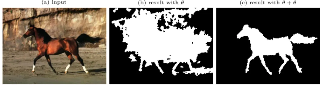
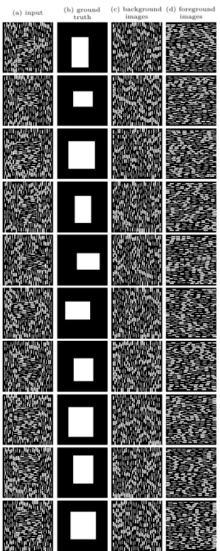
Probabilistic graphical models are nowadays widely used tool in computer vision. Representing an image with the help of a graph together with its neighborhood structure allows us to use graphical models and solve a task related to the image, such as segmentation, labeling or denoising. A common way is to formulate an energy function which describes the fitness of a variable configuration, and then to apply numerical optimization to determine an optimal or at least good solution. For instance let us consider the binary image labeling problem: the aim is to assign each pixel either to a foreground or a background set. Fig.1.1 provides an example where the horse is marked as foreground segment and the remaining pixels as background.
Representing the image labeling problem using graphical models, requires to define a graphG = (V,E) with nodes V representing the image pixels or superpixels and edges E representing neighborhood structures. On this a discrete energy function,
Eθ(x) = X i∈V θi(xi) + X e∈E θe(xe). (1.1)
is defined and solved using a suitable optimization algorithm.
For (1.1) we need to choose parametersθwhich depend on some data feature vectors in the image, which should capture sufficient information of the image structure. However, it is not always straight-forward to choose suitable parameters. Moreover, different choices lead to different results depending on the application at hand. One way is to define the model parameters based on some heuristic. Often this is not a straight-forward task, for instance, when the data has high variances in shape and color as in the Weizmann horse dataset [BU08] visualized in Fig.1.1. While in the first image the horse can be easily segmented from the background with some segmentation algorithm like a minimum cut, this is not the case for the other two images. The second image is quite difficult to be segmented as the head of the horse is not easy to be distinguished from the background behind it, and the same holds for the horse tail. In addition the whole horse region is not homogeneous with respect to color. In contrast, the third image has a homogeneous color in the horse area, but part of the background shares the same color. In particular this part is connected to the horse region. A simple segmentation algorithm would tend to segment this image as horse together with the white background part or merge the horse head and tail with the background for the second image. Hand tunning of the model parameters for each image separately could lead to some reasonable segmentation results. This is, however, time consuming and is not an appropriate solution especially in the case
(a) input
(b) ground truth segmentation
Figure 1.1. -(a) Three images of horses from the Weizmann horse dataset [BU08] with (b) their ground truth segmentation. While the first image can be segmented with some segmentation algorithm, for instance max-flow algorithms which find the minimum cut, the two other images would certainly fail even when powerful features are used. The reason is variances in the foreground class and the similarity of the foreground and background class for the last two images respectively.
1.2. Related Work
when the data to be processed is huge.
A more appropriate way, is tolearn the model parameters, given a set of training data with available ground truth segmentation, e.g. obtained by hand-annotating images. For the case when part of our dataset consists from the three images from Fig.1.1learning model parameters results in model parameters which equally represent the whole dataset. The data on which the model parameters are trained should be representative for the data on which they are tested. Otherwise the segmentation performance will deteriorate.
Based on the learned parameters new model parameters corresponding to the testing data are predicted using some prediction model, e.g. least-squares, Gaussian regression.
Common approach for learning is to define an objective function, or loss function, which depends on the model parameters and measures the prediction error on the training data. After minimizing the function, e.g. using gradient descent-based methods, the learned model parameters are obtained. Computing the prediction error involves minimizing (1.1). As in general (1.1) is NP-hard a relaxed version is considered. Due to this the loss function minimizes error based on approximations. Or in other words by computing “approximate” gradients. Loss functions of this type collect all the training data and learn set of model parameters that best match all data at once. In this fashion the learned set of model parameters might not be able to always reconstruct ground truth for each of the training data.
Part of our work is motivated by the idea of inverse linear programming which corrects a given feasible sub-optimal solution to an optimal one. Our first learning method based on this concept, first corrects the learned approximate gradients computed by a learning method such that it leads to the exact ground truth solution for each of the data in the training set. We will refer to this method as inverse linear programming approach (invLPA). Subsequently any existing model parameter prediction method can be applied to compute a prediction on the testing data.
A further part of this work is dedicated to our second novel objective function for learning, referred as linearly parametrized joint learning approach (LA), which has an objective which is a loss function of the common type as explained above.
1.2. Related Work
The literature of learning in general is vast and and we refer the reader to [NL11] for an excellent overview. Important related work on learning using relaxed inference is the work of Wainwright et al. [Wai06] where it was proven that learning can even benefit from approximations as long as the same approximate inference method is used while learning and predicting. In practice the error introduced while learning approximate parameters is partly compensated by the error of the inexact inference.
The literature on inverse linear programming [ZL96, ZL99, AO01] are the basis for the main novel learning method we present in this work. The authors in [ZL96] apply inverse optimization to the minimum cost flow problem and the assignment problem, which result in a linear program. We follow the same idea and develop
an inverse linear program for the relaxed discrete binary energy function for image labeling.
Most learning methods require the definition of a loss function which steers optimization towards a very small training error. A well known learning method based on such a loss function is structured Support Vector Machine (SVM) [FJ08,
THJA04, TJHA05], a generalization of the classification SVM, and can be applied to different type of data such as lattices, sets and strings. The basic idea is to minimize a problem specific loss function while maximizing the minimal prediction error on the training data.
One of our proposed learning methods leads to a similar objective as the structured SVM. However, our objective is easier to optimize as we fix one of the variables which has a similar role in the structured SVM learning. In addition we use a different optimization method as compared to structured SVM. We use an enhanced subgradient method which involves simpler numerics than a cutting plane method, as used for structured SVM.
Our subgradient method is also known by the name deflected subgradient method. This subgradient method was first proposed in [CFM75] with the aim speeding up the usually slow subgradient method. The PhD work of [Gut03] more thoroughly analyzes the deflected subgradient method proposed in [CFM75]. The authors in [dF09] discuss two approaches for speeding up the subgradient method which tends to advance in zig zag curves. The deflected subgradient method usually comes with a (modified) Polyak step size first proposed by Polyak in [Pol69]. The Polyak step size acquires knowledge of the optimal objective value which is in general not known. Due to this Polyak proposed a modification of this step size when an upper or lower bound of the function is available.
In order to show competitiveness of learning methods we compare our learning method LA based on loss minimizing to two methods from [Dom13], which compares learning methods with different loss functions. Domke compares loss functions based on Maximum a Posteriori Marginal (MPM) to those based on Maximum Likelihood Estimates (MLE) for the learning problem. However, he uses only inference methods based on MPM. Along with a new (heuristic) optimization method he concludes that MPM loss functions lead to better performance than those based on MLE.
Concerning the real world data we use for evaluation of our learning methods we use the challenging Weizmann horse dataset [BU08]. In addition we use the densely annotated video sequence dataset introduced in [PPTM+16].
1.3. Contribution
The main contribution of this work is two novel methods for learning parameters in graphical models.
In addition we propose a new optimization method and apply it to two metric learning approaches which arise from learning suitable distances with aim improving k-means clustering. Metric learning on the other hand can be considered as learning the unary part of the graphical model. We illustrate the proposed method on few
1.4. Organization
small datasets and demonstrate its efficiency with comparison to established solvers for semi-definite programming.
The first proposed learning method, inverse linear programming approach (invLPA), we develop, is using the concept of inverse linear programming. This method corrects the “approximate” gradients of another learning method. We show that the corrected potentials correspond to exact ground truth segmentation.
The second proposed method we develop, the linearized approach (LA) shares some common ideas with structured SVM [FJ08,THJA04, TJHA05] but requires less complex numerics procedure for minimizing the loss function during training. We show how to choose a parameter set by hand which enforces uniqueness. Furthermore, we prove convergence of the deflected subgradient method with modified Polyak step size we use for optimizing the objective of LA.
We evaluate our two learning methods both on synthetic and real world datasets and compare to state-of-the-art classification methods. Furthermore, we illustrate the benefit of learning using an objective function where both a regularizer is present as opposed to training a classifier and adding a regularizer in a post processing step. We extend our methods to learn pairwise potentials and demonstrate that they outperform standard regularizers, e.g. the Ising regularizer, when difficult structures have to be learned. Furthermore, jointly learning unary and pairwise potentials with LA is compared to two other learning methods for parameters in graphical models from [Dom13]. In addition to single images we also consider videos and extend LA to motion segmentation learning and provide experiments on the real world dataset [PPTM+16].
Finally, we discuss the benefits as well as the drawbacks from both learning approaches and propose some possible extensions.
1.4. Organization
We organize this work as follows.
In Chapter 2we introduce all the basic background we use throughout this thesis. We start with definitions from graph theory used in image analysis and proceed with probabilistic graphical models. Next, we present the basic tools from convex optimization in order to proceed with exponential families. The following two sections are dedicated to inference and learning, which are the central tools for solving graphical models. The last section addresses inverse linear programming which is the basis of one of our learning methods presented in Chapter 4.
In Chapter 3we introduce metric learning methods. We give an overview on the most popular approaches and the utilized numerical techniques. In addition, we propose a new optimization procedure which we also apply to two metric learning objectives. We implement our proposed optimization method to few small datasets and compare it to established semi-definite solvers used for metric learning.
In Chapter 4 we develop our two novel methods which can learn both unary and pairwise potentials in a graphical model. We discuss the proposed methods from a theoretical point of view. Also the optimization methods used in LA are
addressed including proofs for convergence. The differences and similarities of LA and structured SVM are discussed. In our experiments we apply invLPA and LA to synthetic and real-world data sets for image segmentation and quantitatively evaluate invLPA with respect to ground truth. Furthermore, we extend the evaluation of LA to semi-supervised online learning in video sequences.
In our last Chapter5we conclude and propose possible extensions of our contribu-tion as further work.
1.5. Notation
The following table provides an overview on the notation used throughout the thesis. Each is introduced in detail in the respective chapter.
Background
G a graphG:= (V,E) which is a pair of a set of nodes (vertices) V, and a set of edges E
X a random variable, a random vector x a value taken by a random variableX
X all possible events of a random variable X, domain of the random variableX
p(x) a probability distribution of the random variable X
(X,G) a probabilistic graphical model, a pair of a random variable X and a graph G
Xi a random variable corresponding to the nodei∈ V from the set of nodesV in the graph G= (V,E) and taking values in Xi
XA := (Xi)i∈A a random sub-vector of X consisting of the ran-dom variablesXicorresponding to the nodes of the setA⊂ V
ij an edge from the edge set E, such thati, j∈ V
C a clique of the graphG= (V,E) which is a subset of the set of vertices V
C(G) set of maximal cliques of the graphG P(V) set of all subsets ofV
fC local function defined on the setC
ϕC(xC) factor or potential indexed with a maximal clique C ∈ C, such thatϕC depends onx only through xC
Z :=R
X
Q
C∈C(G)ϕC(xC)dxpartition function, normalizing con-stant
π(i) the set of all parents of a node i N(i) the set of all neighbors of a node i
1.5. Notation
R :R∪ {∞} the extended set of real numbers
w :E →Rweighting function from the set of the edges E of a graph G= (V,E) to the set of real numbersR
A∪B union of the sets Aand B A∩B intersection of the sets A and B
A\B difference of the sets A and B, elements in the setA which do not belong to the set B
A |=GB|C set C is separating the disjoint sets A and B, for which A, B ⊂ V \C, in the case when the sets are random variables, the relation is for conditional independence ofAandB, given C
φα :X →Rd function called sufficient statistics
θα canonical parameter forφα Θ space of canonical parameters A(θ) :Rd→Rlog-partition function
A∗(µ) :Rd→Rconjugate dual to the log-partition function A
E[f(x)] expected value of a function f(x)
M mean parameter space µα mean parameter
Mo interior of (the mean parameter) space
rint(M) relative interior of (the mean parameter) space M closure of (the mean parameter) space
H :Rd→RShannon entropy
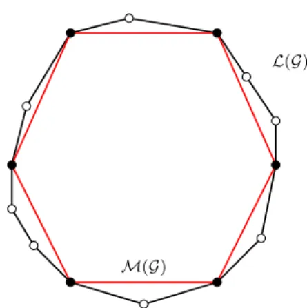
M(G) marginal polytope corresponding to the graph G L(G) local polytope corresponding to the graphG
T a tree-like graph L set of labels
Eθ energy function corresponding to a distribution with canoni-cal parameters θ
[n] ={1,2, ..., n}set of all natural numbersisuch that 1≤i≤n [.] Iverson bracket, 1 if the value in the bracket is true and 0
otherwise IA(x) =
(
0 ifx∈A
+∞ ifx6∈A , indicator set function on a setA KL Kullback-Leibler divergence
N set of natural numbers
||x|| =p
hx, xi Euclidean norm forx∈Rn hx, yi =Pn
i=1xiyi inner product in the Euclidean space,x, y,∈Rn Sd+ cone of symmetric positive semi-definite matrices
conv(A) convex hull of a set A⊂Rn aff(A) affine hull of a set A⊂Rn
B(x, ε) open Euclidean ball
epi(f) epigraf of a function f
∇f gradient of a functionf ∇2f Hessian of a functionf
S−(f, c) sublevel set of a function f S+(f, c) superlevel set of a function f
Metric Learning
G a graphG:= (V,E) which is a pair of a set of nodes (vertices) V, and a set of edges E
S indices of similar pairs of points D indices of dissimilar pairs of points
R :={(i, j, k)|xi is more similar to xj than toxk}
M an arbitrary matrix in Rn×n
l(M,D,S,R) a loss function r(M) a regularizer function
Sn+ cone of symmetric PSD n×n real-valued matrices
I identity matrix tr(M) trace of a matrixM
dM(xi, xj) :=h(xi−xj), M(xi−xj)i1/2 distance metric with respect to a matrix M Xij := (xi−xj)(xi−xj)T XS :=P(xi,xj)∈SXij XD :=P(xi,xj)∈DXij 4|D|−1 :={u∈R|D| ui ≥0, Pn i=1ui= 1}the (|D| −1) dimensional probability simplex ˜ M :=XS1/2M XS1/2 ˜ Xij :=X −1/2 S XijX −1/2 S P :={M|M 0 and tr(M)≤1} C :={M˜ 0 : tr( ˜M) = 1} ⊗ Kronecker product
I :R→R an indicator function defined byI(x) :=
(
0 ifx≥0 ∞ ifx <0 Model Parameter Perturbation and Learning
Eθ(x) discrete energy function with potentialsθ(x)
G a graphG:= (V,E) which is a pair of a set of nodes (vertices) V, and a set of edges E
L the set of labels µ vector of assignments
µ∗ vector of assignments corresponding to groundtruth segmen-tation
1.5. Notation
LM
G local polytope defined on a graphGcorresponding to minimal representation
ˆ
θ intial potentials ˜
θ := ˆθ+θ corrected potentials
w := (wu, wp)> parameter vector, where wu is the part corre-sponding to the unary potentials andwp the part correspond-ing to the pairwise potentials
Θ(µ∗) :={θ˜∈Rm+n|minµ∈LM G h
˜
θ, µi=hθ, µ˜ ∗i}set of model param-eters that correspond to ground truth assignments
fi feature vector corresponding to unary term fij feature vector corresponding to a pairwise term k(fi, fj) :=σ2mexp−2σ12 f kfi−fjk2, withσ2 f,σm2 parameters K(F) := k(fi, fj) i,j∈[N]
θφ :=θ−A>φ, whereAis the matrix corresponding to the local polytope equations and φis a dual variable vector
L(w) := maxµ∈LG
h−θ˜w, µi+hθ˜w, µ∗i loss function for the LA method, in the case when there is one training image L upper bound on the loss function L
gkk≥0 sequence of subgradients
fkk≥0 sequence of deflected subgradients PS projection on a set S
αk step size in subgradient method % mis 100
P
p(I(p)6=Igt(p))
|p| percentage of all mislabeled pixels, I is the obtained segmented images, Igt is the ground truth seg-mentation and |p|is the number of pixels
% mis fg 100Area(F∩Fgt)
Area(F∪Fgt) percentage of mislabeled foreground pixels,
Fgt is the ground truth foreground mask and F is the fore-ground mask of the obtained segmented image
2. Background
This chapter will introduce all necessary tools which are required in the remainder of this thesis.
We organize the chapter as follows: in Sect. 2.1 we start with the fundamental concepts and definitions of graphs and probabilistic graphical models. Next, in Sect. 2.2 we include brief overview on some basic concepts in convex analysis and optimization. In Sect. 2.3 we consider the concept of exponential families which provide a theoretical basis for probabilistic graphical models when interpreted as exponential family models. Considering a graphical model as an exponential family member allows us to use convex analysis when exploring graphical models. We apply these concepts to two of the most important basic problems in computer vision, inference in Sect.2.4and learning in Sect.2.5, while exploiting the theory of exponential models. In Sect.2.6we address inverse linear programming which is the most important concept used in this thesis.
2.1. Graphical Models
Graphical models or probabilistic graphical models are tools for modeling probabilistic relations between random variables using a graph-like structure. Graphical models are a widely used tool in computer vision, statistics, machine learning and many other fields in science.
We first introduce the basic concepts and definitions in graph theory, most of which we use throughout this work. Next we continue with probability theory which provides the basis for learning probabilistic graphical models.
2.1.1. Graph Theory Used in Image Processing and Analysis Let us first define what a graph is, [Die12].
Definition 2.1.1. A graph is an ordered pair G = (V,E) consisting of a set of objects represented as nodes (vertices)V, together with binary subsets of distinct nodes, represented by a set of edges,E ⊂ {ij∈ V × V |i6=j}.
Each edge in the graph represents some relation between two nodes. The edge ij is referred to as directed edge ifij 6=ji. A graph with undirected edges is referred to asundirected graph and as directed graph otherwise.
A path is a sequence of distinct nodes, in which the sequent nodes are adjacent in the graph G. A path from a node to itself which contains each node and edge not more than once, is called a cycle. A graph is either a cyclic graph if it containts at least one cycle or an acyclic graph otherwise. An edge between two nodes of
one cycle, which is not part of the cycle is called a chord of the cycle. A chordal graph or triangulated graph is an undirected graph G= (V,E), for which every cycle with length greater than three has a chord. A directed graph with no directed cycles is calleddirected acyclic graph (DAG).
Aclique C in an undirected graph G = (V,E) is a subset of the set of vertices C ⊂ V, such that there is an edge between each of the vertices in C, that is ∀i, j∈C, i6=j :ij ∈ E. A maximal clique is a clique which can not be extended by adding a further node. We denote the set of maximal cliques of a graphG with C(G).
Node iis called a child of a nodej, and a nodej is a parent of a node i, if there exists a directed edge fromj toi. We denote the set of all parents of a node iwith π(i). Neighbors of a node iare all nodes which are connected to the nodeiby an edge, that is,N(i) :={j∈ V |ij∈ E}.
In a connected graph for each node there exists a path to all other nodes. A
tree is an acyclic undirected connected graph. If an acyclic undirected graph is not connected then the graph is called aforest or union of trees. A spanning tree of an undirected graph is a subgraph forming a tree which includes all vertices and a minimum number of edges ofG.
Any acyclic directed graph can be transformed into an undirected graph. This transformed undirected graph is calledmoral graph.
Definition 2.1.2. An undirected graph G = (V,E) in which all parents of each child are linked, and all directed edges are converted into undirected ones is called a
moral graph.
With assigning a weight function w :E →R to the graph, so that each edge ij gets a weightwij, the graph G= (V,E, w) is called weighted graph.
A graphG is said to beconnected if there is a path between every pair of vertices inG. A graph which is not connected is said to bedisconnected.
Definition 2.1.3. In an undirected connected graph G= (V,E),C ⊂V is said to be acut orseparating set of G if removing it renders the graph disconnected. C separating two disjoint setsA, B⊂ V \C, inG is denoted withA |=GB|C.
Definition 2.1.4. (A, B, C) is a proper decomposition of an undirected graph G= (V,E) into three disjoint subsets A, B, C⊂ V,A∪B∪C=V such that C is a clique ofG which separatesA and B.
A decomposable graph is one for which there exists a sequence of proper decomposi-tions such that all subsetsAandB are cliques inG. An undirected graphG = (V,E) is decomposable if and only ifG is triangulated, see [CDLS07, Theorem 4.4].
Aclique tree is an acyclic undirected graph whose nodes are formed from the maximal cliques of an undirected graphG, which can be cyclic. For an undirected graphG which is decomposable there always exists a junction tree which is a clique tree with a special property.
Definition 2.1.5. A junction tree of an undirected graph G is a clique tree, so that for any two cliques Ca and Cb, their intersectionCa∩ Cb is contained in every clique on the unique path joining them.
2.1. Graphical Models
2.1.2. Probabilistic Graphical Models
A probabilistic graphical model is a graphical model G = (V,E) with a random variable X vector, composed of variables Xi taking values xi ∈ Xi, ∀i ∈ V. The edge set E is used to imply conditional independences on X and to factorize the underlying probability distribution p(x) with respect to some measure. We will use the same notation p(x) for the density function and the probability distribution of a random variable X, having a valuex, that is we denote P(X=x) =p(x), which is in fact the case for the discrete setting.
For a continuous random variable, the integral of the probabilities of all events have to be one, that is R
Xp(x)dx = 1, while for a discrete random variable the probabilities of all events have to sum up to one, that isP
x∈Xp(x) = 1. Theexpected
value of a functionf(x) for a continuous random variable is defined asEp[f(x)] :=
R
x∈Xp(x)f(x)dxand for a discrete random variable asEp[f(x)] :=Px∈Xp(x)f(x). For some subsetA⊂ V, themarginal distributionof the corresponding continuous variables isp(xA) =RXV\Ap(x)dxV\A and in the case of discrete variables,p(xA) =
P
xV\A∈XV\Ap(x). For two disjoint subsets A, B⊂ V the conditional distribution
of a random vector XA, given the observed random vector XB, with p(xB)>0 is given with theBayes’ rule [Bay63]
p(xA|xB) = p(xA, xB) p(xB) = p(xB|xA)p(xA) p(xB) . (2.1)
Let A, B, C be disjoint subsets ofV. The random vectorsXA andXB are called
conditionally independent, givenXC withp(xC)>0, denoted withXA |=XB|XC if and only if the joint conditional distribution can be written as the product of their marginal conditional distributions, that is
XA |=XB|XC ⇔ ∀xA∈ XA, xB ∈ XB, xC ∈ XC :p(xA, xB|xC) =p(xA|xC)p(xB|xC). (2.2) The ternary relation X |=Y|Z satisfies the following properties
symmetry ifX |=Y|Z thenY |=X|Z (2.3a)
decomposition ifX |= (Y, Z)|W thenX |=Y|W (2.3b)
weak union ifX |= (Y, Z)|W thenX |=Y|(Z, W) (2.3c)
contraction ifX |=Y|(Z, W) and X |=W|Z thenX |= (Y, Z)|W. (2.3d) If the probability distributions p over the random variablesX, Y, Z, W are strictly positive then the following additional property holds too
intersection ifX |=Y|(Z, W) and X =|W|(Y, Z) thenX |= (Y, W)|Z. (2.4a) The notion of a graphical model can be explained using the conditional independences between random variables. Moreover, a graph can be thought as a map of conditional independences between random variables. We consider the following definition of a probabilistic graphical model, valid for both directed and undirected graphical
models :
Definition 2.1.6. A probabilistic graphical model is a pair (X,G) of a random vector X and a graph G with a probability distribution p(x). Every conditional independence statement implied byG is satisfied by p(x), that is for A, B, C ⊂ V, A |=GB|C =⇒ XA |=XB|XC. The graph G implies conditional independences between random variables, called Markov property. Moreover the graphG implies factorization of the probability distribution with
p(x) = Y C∈C
fC(xC) (2.5)
whereC ⊂ V andC ⊂ P(V), whereP(V) is the set of all subsets ofV, and fC are local functions defined on the subsetsC⊂ V.
In the next subsections we give a more precise definition in the sense of the factorization of the probability function when the graphical model is directed and undirected.
2.1.3. Directed Graphical Models: Bayesian Networks
Directed graphical models also referred to as Bayesian networks, make use of the Bayes’ rule to factorize the probability distribution such that each factor represents a causal relation of the model, leading to a directed acyclic graph. This relation in directed graphical models is represented by a directed acyclic graph.
Definition 2.1.7. Adirected graphical model (X,G) is a pair of a random vector X and a directed acyclic graphG = (V,E), so that the joint probability distribution p(x) ofX can be factorized as product of local conditional distributions
p(x) =Y i∈V
p(xi|xπ(i)), (2.6)
where with π(i) we denoted the set of all parents of a node i.
2.1.4. Undirected Graphical Models: Markov Random Fields (MRF) When the graph structure in the probabilistic graphical model is undirected then the graphical model is commonly called Markov random field (MRF). We first give the definition of an undirected graphical model with respect to the separation property, see Definition2.1.3.
Definition 2.1.8. Anundirected graphical model (X,G) is a pair of a random vectorX and an undirected graph G= (V,E) so that if two disjoint subsets A, B⊂ V \C are not connected in GV\C, thenXA |=XB|XC.
The relations between the edge setE of a graphG and the random variables are given by the Markov properties of the random variables defined next.
2.1. Graphical Models
Definition 2.1.9. Markov Properties: For an undirected graphical model (X,G) we say that X has the
(G) global Markov property with respect toG, if for any three disjoint subsets A, B, C ⊂ V for which A and B are separated by C, XA |=XB|XC holds. This property is satisfied for any undirected graphical model, due to Definition2.1.8.
(L)local Markov propertywith respect toG, if∀i∈ V,Xi |=XV\({i}∪N(i))|XN(i)
holds, where N(i) denotes the neighborhood ofi.
(P)pairwise Markov property with respect toG, if for all pairs of non-adjacent nodesiand j,Xi =|Xj|XV\{i,j} holds.
If in addition to (G) the probability distributionp(x) is strictly positive,p(x)>0 ∀x∈ X, then both (L) and (P) hold for the undirected model (X,G), that is (G) is equivalent to (L) and (P), see [Lau96,CDLS07].
For undirected graphical models there is also a factorization rule of p(x), which is different than the one for directed graphical models.
Definition 2.1.10. For an undirected graphical model (X,G) the probability distri-bution p(x) of the random vector X factorizes as
p(x) = 1 Z Y C∈C(G) ϕC(xC) and Z = Z X Y C∈C(G) ϕC(xC)dx (2.7)
where ϕC are called factors or potentials, indexed with the maximal cliques
C⊂ C(G) andϕC depends onxonly throughxC. The normalizing constantZ is also refered to aspartition function and ensures that the integral of the probabilities of all events is 1.
It can be shown that if X has the factorization property with respect to an undirected graphG, then X has the global Markov property. The reverse holds in the case of strict positivity of p(x)∀x∈ X. This is stated in the following theorem known as Hammersley-Clifford theorem [HC71].
Theorem 2.1.1. Hammersley-Clifford : A random vector X with a strictly positive probability distribution, that isp(x)>0∀x∈ X satisfies the pairwise Markov property with respect to an undirected graph G if and only if it factorizes with respect toG as in (2.7).
Proof. See [LS03, Theorem 3.9].
In general, the conditional independence properties for undirected graphical models are much simpler than those for directed graphical models. We saw that a directed acyclic graph can be transformed into an undirected one using moralization, see Definition2.1.2. However, during this transformation some information on conditional independence of variables is lost. On the other hand a subclass of undirected graphs, undirected graphs with chordal graph structure, can be transformed into an equivalent directed one. For details we refer the reader to [KF09].
2.2. Basic Concepts in Convex Analysis and Optimization
In this section we want to introduce basic concepts of convex analysis and optimization which will be used throughout this thesis. For more detailed introduction on convex optimization we refer to [Roc70,BV04].In practice, solving an optimization problem can be very difficult or not possible at all. However, when the problem is convex, the situation might become better. This is also a cause by the fact that convex optimization problems have been studied a lot in the past and there is a huge literature on how to deal and solve efficiently convex problems. However, the key property of a convex problem is that local optimizers are always global ones.
2.2.1. Convex Sets
We start by defining convex sets.
Definition 2.2.1. A setA ⊆Rn is convex if for all x, y∈A and 0< α < 1, the pointαx+ (1−α)y∈A.
Theintersection ∪i∈IAi of a family of convex sets{Ai}i∈I for an arbitrary index setI is also a convex set. TheCartesian product A1⊗A2⊗...⊗An of a family of convex sets{Ai}i∈I as defined above is a convex set as well. However, the union of convex sets is not necessarily a convex set.
Definition 2.2.2. A set K⊂Rn is called a coneif for all x∈K, the ray{λx|λ > 0} ∈K. IfK is convex then the cone K is called a convex cone.
The cone of symmetric positive semi-definite matrices is defined by
Sd+ :={X∈Rd
×d|X=X>
, X 0}. (2.8)
Similarly withSd++we denote the cone of positive definite matrices
Sd++:={X∈Rd×d|X=X>, X 0}. (2.9)
Theorem 2.2.1. Farkas-Minkowski-Weyl: A cone is polyhedral if and only if it is finitely generated.
Proof. For proof see [Sch98, Corollary 7.1a].
A polytopeis the convex hull of its vertices or extreme points. Definition 2.2.3. The convex hull of a setA⊂Rn is defined as
conv(A) := ( n X i=1 αixi|A={x1, x2, ..., xn}, αi ∈R, αi ≥0, n X i=1 αi = 1 ) . (2.10)
Definition 2.2.4. The affine hull of a set A⊂Rn is defined as
aff(A) := ( n X i=1 αixi|A={x1, x2, ..., xn}, αi∈R, n X i=1 αi= 1 ) . (2.11)
2.2. Basic Concepts in Convex Analysis and Optimization
Due to more restrictions the convex hull is always a subset of the affine hull. Definition 2.2.5. An−1 dimensionalsimplex∆n−1 is an−1 dimensional polytope
which is a convex hull of its ndimensional vertices ∆n−1 :={u∈Rn:ui≥0,
n
X
i=1
ui= 1}. (2.12)
The simplex has one dimension less than the space in which it is embedded due to the constraint that the sum of all its vertices has to sum to one, and so one of the n vertices can be expressed using the restn−1, which makes it one dimension less thanRn.
Definition 2.2.6. For ε >0 and x∈Rn the open Euclidean ball is defined by
B(ε, x) :={y∈Rn| ||y−x||< ε}. (2.13)
Definition 2.2.7. The interior of a convex set A⊂Rn is defined by
Ao:={x∈A| ∃ε >0 :B(ε, x)⊂A}, (2.14) where B(ε, x) is the Euclidean ball as defined in Definition 2.2.6.
Definition 2.2.8. The relative interior of a convex set A⊂Rn is defined by rint(A) :={x∈A| ∃ε >0 s.t. B(ε, x)∩aff(A)⊂A}, (2.15) with B(ε, x) as defined in Definition 2.2.6.
The interiorAoand relative interior rint(A) of a convex setA⊂
Rnare also convex
sets and rint(A) is always nonempty, i.e. rint(A) 6= ∅. A convex set A ⊆ Rn is full-dimensional if aff(A) =Rn. IfA is full-dimensional then rint(A) =Ao.
An important function we will use is the set indicator function defined on a set A⊂Rnby
IA(x) :=
(
0 ifx∈A
+∞ ifx6∈A. (2.16)
When A is convex then IA is convex too. Indicator functions of convex sets are of interest in constrained convex optimization. With their help, a constrained optimization problem can be converted into an unconstrained one. As a consequence we can treat both constrained and unconstrained convex problems in a unified way. 2.2.2. Convex Functions
Definition 2.2.9. A function f :Rn→R isconvex if
f(αx+ (1−α)y)≤αf(x) + (1−α)f(y) (2.17) holds for all x, y∈Rn and 0< α <1.
The domain of the function f is defined by
domf :={x∈Rn|f(x)<∞}. (2.18) Functionf :Rn→Ris convex if and only if theepigraf of f defined by
epi(f) :={(x, y)∈Rn×R|f(x)≤y} (2.19)
is convex.
Definition 2.2.10. A functionf :Rn→Risstrongly convex on some setA⊂Rn if there existsm >0 such that
∇2f(x)mI (2.20)
withI the identity matrix.
Definition 2.2.11. A convex functionf is calledproper iff is finite for at least one point, that is domf 6=∅.
Continuity
A function f is lower semi-continuous if for any sequence {xk}k ⊂Rn so that
{xk}k→x∈Rn
f(x)≤lim inf
k→∞ f(xk). (2.21)
Similarly f is upper semi-continuous if for any sequence {xk}k ⊂ Rn so that
{xk}k→x∈Rn
f(x)≥lim sup k→∞
f(xk). (2.22)
Iff is both lower semi-continuous and upper semi-continuous thenf iscontinuous. Definition 2.2.12. A function f :Rn→R iscontinuous relative to some convex setA⊂Rn if the restriction off toA denoted by f|A is a continuous function.
A stronger notion for the relative continuity is given by the following definition. Definition 2.2.13. A functionf :A→Ris calledLipschitz continuous relative
toA⊂Rn if there existsL≥0 such that
||f(x)−f(y)|| ≤L||x−y|| (2.23) wherex, y∈A.
We will see that Lipschitz continuity of the gradient of f is the key ingredient for convergence guarantees of some optimization algorithms, including the gradient descent.
2.2. Basic Concepts in Convex Analysis and Optimization
Duality
For a proper function f : Rn → R its conjugate dual or Legendre-Fenchel conjugate dual functionf∗:Rn→Ris defined by
f∗(y) := sup x∈Rn
{hx, yi −f(x)}. (2.24) The dual is always a convex and lower semi-continuous function even if the function f is not convex.
Definition 2.2.14. A convex differentiable functionf, isessentially smooth, if it has a nonempty domainA= dom(f),f is differentiable onAoand limk→∞∇f(xk) = ∞ for any sequence {xk}k∈A, limk→∞xk=µ, where µis a boundary point ofA.
A convex function f with dom(f) =Rn is essentially smooth since its domainRn
has no boundaries.
Differentiability
A convex function is not necessary differentiable. For this reason the notion of differentiability is generalized and to this end the notionsubdifferential of a proper functionf :A→R,A⊆Rn is introduced and defined as
∂f(x) :={w∈A|f(y)≥f(x) +hw, y−xi,∀y∈A}. (2.25) For a convex differentiable f at x the set of subdifferentials at xconsists of a single element which is exactly the gradient ∇f. When f is lower semi-continuous, then the set of subdifferentials off is always nonempty, see [Nes04, Theorem 3.1.13 ]. Proposition 2.2.2. A differentiable function f :A→R, where A⊂Rn is open, is
convexif and only if for all x, y∈A
f(y)≥f(x) +∇f(x)>(y−x) (2.26) is satisfied. If the inequality is strict whenever x6=y, f is strictly convex.
Proof. For proof see [BV04, Sect. 3.1.3].
Proposition 2.2.3. For a twice differentiable function f :A→Rn where A⊂
Rn
is convex and open, f is convex on A if and only if the Hessian of f defined by
∇2f(x) := ∂ 2f ∂xi∂xj (x1, ..., xn) ! i,j∈[n] , x= (x1, .., xn)> (2.27) is positive semi-definite ∀x∈A.
Sublevel set
Definition 2.2.15. The sublevel set of a functionf is defined as
S−(f, c) ={x∈dom(f)|f(x)≤c} (2.28) and thesuperlevel set accordingly as
S+(f, c) ={x∈dom(f)|f(x)≥c}. (2.29)
For an initial point x0 of an iterative algorithm, it should be always satisfied that the point is in the domain of the functionx0 ∈dom(f) and the sublevel set of the functionf should be closed. Sublevel sets are important for analyzing convergence of some algorithms like gradient descent: based on the condition number of the Hessian of the function on the sublevel set, the speed of convergence of gradient descent can be determined.
2.2.3. Gradient Descent Method
Gradient descent is a first order method for optimizing a differentiable convex function. Every next iterate is computed in the direction of the negative gradient and with an appropriately chosen step size. For a convex differentiable functionf :RN →R, let xi be the current iterate, then the next iterate is given by
xi+1=xi−λi∇f(xi) (2.30)
whereλi is a step size appropriately chosen in every iteration. For a descent method we demand that the function value is decreased in every step, i.e.
f(xi+1)< f(xi) (2.31)
until the optimalx∗ is reached. Due to convexity off, from Proposition2.2.2with y = xi+1 and x = xi and using the previous inequality (2.31) we require for the variable update:
∇f(xi)>(xi+1−xi)<0. (2.32) The convergence of the gradient descent depends on the choice of the step size λi. Convergence can be proved when∇f is Lipschitz continuous with Lipschitz constant L≥0, if 0<infiλi ≤supiλi< L2, see [Nes04].
Line Search Methods
Line search methods search along the line direction for the next iterate, thus de-termining a step size. In theory, they aim at finding a global minimum of the function
2.2. Basic Concepts in Convex Analysis and Optimization
where λi > 0. Computing this global minimum is in general very expensive and requires computation of the gradient of g in each step. Due to this, line search methods are more efficient when they search only for an approximation to this global minimum or just a sufficient reduction off in the next iterate.
Line search methods work such that some condition which implies decrease of the function in the next iterate is satisfied. We present the most commonly used conditions in line search methods.
An inexact line search method is said to satisfy the Wolfe conditions if the following constraints are fulfilled:
Armijo condition :f(xi+λi∇f(xi))≤f(xi) +c1∇f(xi)>∇f(xi) (2.34a)
curvature condition:∇f(xi+λi∇f(xi))>∇f(xi)≥c2∇f(xi)>∇f(xi) (2.34b)
where 0< c1, c2<1. The Wolfe conditions are a set of conditions which guarantee
sufficiently fast convergence of the gradient descent method. The Armijo condition guarantees sufficient decrease of the function, while the curvature condition excludes short step size which slows down the optimization process. Stronger conditions than the Wolfe conditions are thestrong Wolfe conditions which include the Armijo condition (2.34a), and instead of the curvature condition (2.34b) the strong Wolfe condition given by
|∇f(xi+λi∇f(xi))>∇f(xi)| ≥c2|∇f(xi)>∇f(xi)| (2.35)
with 0 < c2 < 1. The strong Wolfe condition assures the iterate to be in the
neighborhood of the global optimum of (2.33).
For a function which is differentiable and bounded from below there always exists a step length λi so that the Wolfe conditions are satisfied. This is shown in the next Proposition.
Proposition 2.2.4. Let f :Rn→ R be continuously differentiable and let ∇f(xi) be the descent direction atxi.Let us also assume that f is bounded from below along the ray {xi +λi∇f(xi)|λi > 0}. Then for 0 < c1, c2 < 1 there exist intervals of
step lengths satisfying the Wolfe conditions from (2.34) as well as the strong Wolfe conditions (2.34a) and (2.35).
Proof. For proof see [NW06, Lemma 3.1].
Commonly used inexact line search method, backtracking line search works by decreasing the step size λi from unit length to λi =βλi, where 0< β <1, until the Armijo condition (2.34a) with 0< c1 <0.5 is satisfied. Backtracking line search can
be used for choosingλi for the gradient descent method. It is commonly used with the damped Newton method (we will shortly briefly describe it) when there is no guarantee for global convergence.
2.2.4. Subgradient Method
The subgradient method is an optimization algorithm developed first by Shor [Sho85] to minimize non differentiable convex functions. We refer to [Ber99] and [Boy14] for more on subgradient methods.
For the subgradient method a different approach is chosen for selecting the step size. The subgradient direction is not a descent direction, and so the function is not guaranteed to decrease with the next iterate. For a convex functionf :RN →R, let xi be the current iterate, then the next iterate with subgradient method is given by xi+1 =xi−λig(xi) (2.36)
where λi is the step size at the i−th iterate and g is some subgradient of f at xi, that isg(xi)∈∂f(xi) as defined in (2.25). The subgradient direction at an iteratei is given by the negative subgradientg(xi). In the case of a differentiable functionf the subgradient direction is the gradient descent direction.
Even though the subgradient method is not a descent method, an important property that makes the subgradient work is that for certain step size choices the distance from the current iterate to the optimal one is reduced in every step. This is a result from the following Proposition:
Proposition 2.2.5. Let the iteratexi be not the optimal one. Then for every optimal solution iterate x∗, we have
||xi+1−x∗||<||xi−x∗||, (2.37)
for all step sizes λi such that
0< λi < 2(f(x
i)−f(x∗))
||g(xi)||2 . (2.38)
Proof. For proof see [Ber99, Proposition 6.3.1].
From the proposition above the range of appropriate step sizes can be known when the optimal valuef(x∗) is known. However in the case when this value is not known, an approximation can be used. Using the result from the Proposition above and an approximate estimation of the optimal valuef(x∗) allows one to use certain step size choices. For more on how the most common step size choices, were developed we refer to [Ber99, Sect. 6.3.1]. Among the most common step sizes used are: constant step sizewhen
λi = const ∀i, (2.39)
constant step length when
λi = const ||g(xi)||
2
![Figure 1.1. - (a) Three images of horses from the Weizmann horse dataset [BU08] with (b) their ground truth segmentation](https://thumb-us.123doks.com/thumbv2/123dok_us/11107643.2998514/18.892.171.682.371.742/figure-images-horses-weizmann-horse-dataset-ground-segmentation.webp)
![Table 3.1. - Classification errors in percentage on the toy data we generate, the iris dataset [Fis36] and the wine dataset [Lic13]](https://thumb-us.123doks.com/thumbv2/123dok_us/11107643.2998514/90.892.131.722.698.852/table-classification-errors-percentage-data-generate-dataset-dataset.webp)