Coding Textual Inputs Boosts the Accuracy of Neural Networks

1350

Coding Textual Inputs Boosts the Accuracy of Neural Networks

Abdul Rafae Khan?_{, Jia Xu}?∗_{, and Weiwei Sun}†

?_{Department of Computer Science, Stevens Institute of Technology}

{akhan4, jxu70}@stevens.edu

†_{Department of Computer Science and Technology, University of Cambridge}† [email protected]

Abstract

Natural Language Processing (NLP) tasks are usually performed word by word on textual inputs. We can use arbitrary symbols to rep-resent the linguistic meaning of a word and use these symbols as inputs. As “alterna-tives” to a text representation, we introduce Soundex, MetaPhone, NYSIIS, logogram to NLP, and develop fixed-output-length coding and its extension using Huffman coding. Each of those codings combines different charac-ter/digital sequences and constructs a new vo-cabulary based on codewords. We find that the integration of those codewords with text pro-vides more reliable inputs to Neural-Network-based NLP systems through redundancy than text-alone inputs. Experiments demonstrate that our approach outperforms the state-of-the-art models on the application of machine translation, language modeling, and part-of-speech tagging. The source code is available athttps://github.com/abdulrafae/coding nmt. 1 Introduction

We introduce novel coding schemes on the inputs of Neural-Network-based Natural Language Pro-cessing (NN-NLP) that significantly boost the accu-racy in three applications. The inputs of NN-NLP rely on observable forms of mental representations of linguistic expressions, and allow alternative de-signs. For example, both logographic kanji and syllabic kana represent Japanese words, and emoti-cons and emojis can express sentiments. These showcase that alternative human language repre-sentation than text is possible and highlight a com-mon belief of most linguists: the relationship be-tween the mental representations and their phono-logical forms is highly arbitrary, even though a

∗

Jia Xu is the corresponding author of this paper. †

This work was completed when Weiwei Sun was at Peking University.

non-arbitrary (de Saussure,1916) mapping exists

for some special cases, e.g., the bouba/kiki effect.

In our work, we ask –Are there alternative forms

of mental representation in addition to text as we

see in Japanese and Internet languageto help

lan-guage understanding in NN-NLP?

To answer this question, we blend concepts from linguistic phonetics, grammatology, and the statis-tics of Zipf law to find alternative language repre-sentations to text. More precisely, we code a textual word either naturally or artificially by exploring dif-ferent facets of human languages, from phonetic and logogram codings to new coding constructions generalizable to all languages. Natural codings in-spire the finding of artificial codings, which in turn helps us understand and explain natural codings.

All of our codings reinforce NLP inputs by re-constructing the character/symbol sequence of a word in various ways with a new alphabet. These variants and their “decomposition” are expressive because they contain insightful information about linguistic patterns in units smaller than words and even smaller than characters. For example, in the logogram Wubi (that lists in a coded form the strokes caligraphing a Chinese character), “众” (crowd) is coded as “www”, which is made of three

“人” (person, “w”), and “从” (follow, “ww”) is a

composition of two “人”. A representation

con-taining such granular details potentially reveals the semantic structure and linguistic meanings inside a word, thus enriching text and allowing a redun-dancy that ensures more reliable NLP inputs.

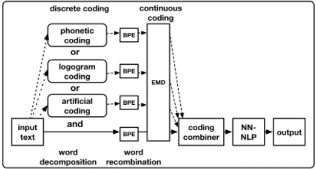
Now that we have put our previous question in context let us give an overview of how we incor-porate coding schemes into an NLP framework in

Figure1. For an input sentence, we apply an

al-ternative coding scheme word by word, then use Byte-Pair-Encoding (BPE) to recombine these sym-bols (to shorten the input lengths), and finally per-form embeddings (EMD). In contrast to word

em-phonetic coding logogram coding artificial coding input text coding combiner NN-NLP and or or output word decomposition word recombination EMD continuous coding BPE BPE BPE BPE discrete coding

Figure 1: Workflow on how to apply discrete coding in NN-NLP by decomposing (phonetic, logogram, fix-output-length, or Huffman coding) and recombining (BPE) words.

beddings that map words to real number vectors, our coding range is discrete. The coded sentence and its original textual input are then combined in three ways: concatenation, linear-interpolation at the encoder level, and multi-source encoding with or without Bi-LSTM, attention, and multi-head at-tention. The combined input is fed into NN-NLP models as a black-box to decode outputs. Our ap-proach is language-, task-, and system-independent and does not use any additional information besides our algorithms.

We conduct experiments on three NLP applica-tions and five languages, including (1) Machine Translation (MT) on English-German, German-English, English-French, French-German-English, and Chinese-English; (2) Language Modeling (LM) on English; and (3) Part-of-Speech (POS) Tagging on English. Our approach significantly and consis-tently improves over state-of-the-art neural models: Transformer, ConvS2S, XLM, and Bi-LSTM with attention mechanisms.

In summary, our contribution mainly lies in the three consecutive folds:

1. Phonetic, logogram, and artificial codings.

We introduce a variety of language repre-sentations by coding words through various schemes of Soundex, NYSIIS, Metaphone, Pinyin, Wubi, fixed-output-length, and Huff-man codings, and propose different ways to

incorporate them in NLP models.（§2)

2. Synergistic coding. We introduce effec-tive ways of combining the textual inputs and their codewords with the state-of-the-art neural network architectures: concatenation, linear-interpolated encoder, and multi-source encoding with or without Bi-LSTM, attention,

and multi-head attention. (§3)

3. NLP Applications. Our method is generaliz-able to different languages and can be applied to any NN-NLP system. Experiments demon-strate that our methods improve over the state-of-the-art models (Transformer, XLM, and ConvS2S) on various tasks in applications in-cluding machine translation, language model-ing, and part-of-speech tagging. (§4)

2 Coding Words

We view each coding as a function γ that maps

a textual word from x ∈ _V, a natural language

vocabulary, into a codewordγ(x)∈ V, a codeword vocabulary:

γ :V→ V (1)

For simplicity of exposition we will considerV to

be the image ofVunderγ. Each codewordγ(x)is

a non-emptyσ-string over the alphabetΣof this

coding:γ(x) =σ1, σ2, σ3· · ·σLwith code length

L. Σ+is an infinite set of all possible non-empty

strings overΣ, andV ⊆Σ+_.

As an example (albeit one which is practi-cally not useful) consider the mapping of four

English words to three binary codewords: V =

{“to”,“be”,“or”,“not”}, Σ = {0,1}, Σ+ =

{0,1,00,01,10,11,· · ·},V = {00,01,11}, L = 2, γ(“to”) = 00, γ(“be”) = 01, γ(“or”) = 11, γ(“not”) = 01,|_V|= 4, and|V|= 3.

To instantiate this function, we start by introduc-ing several existintroduc-ing lintroduc-inguistically-motivated codintroduc-ing schemes (and later on we will extend this to new coding schemes we develop): the phonetic and lo-gogram coding as surjective functions, where in particular|_V| ≥ |V|; and the fixed-output-length and Huffman coding as bijections, where|V|=|V|.

In traditional coding theory, a compression code has to be injective in order to be uniquely decod-able. In our work, we only care about the task-specific prediction and not in decoding the orig-inal message. Therefore, we relax the injective restriction on the codings to deviate a little from the standard typical coding theory applications for technical convenience.

Throughout this paper, we choose to name the

functionγ as “coding” (although sometimes it is

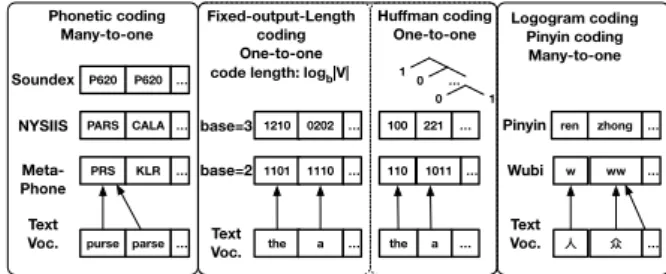
also called “encoding”) to distinguish from the en-coder in the NN-NLP models. An overview of our coding schemes is illustrated in Figure2.

Meta-Phone P620 P620 … PARS CALA … PRS KLR … NYSIIS Soundex Text

Voc. purse parse …

Phonetic coding Many-to-one base=2 1210 0202 … 1101 1110 … base=3 Text Voc. the a … Fixed-output-Length coding One-to-one 100 221 … 110 1011 … the a … Huffman coding One-to-one 1 0 … 0 1

code length: logb|V|

Wubi w ww … Text Voc. ! " … Logogram coding Pinyin coding Many-to-one

Pinyin ren zhong …

Figure 2: Examples on different coding schemes. In contrast to Pinyin only applies to Chinese, the lo-gogram coding Wubi and its variant apply to Japanese Kanji and Chinese. Furthermore, phonetic codings, in-cluding MetaPhone, Soundex, and NYSIIS, cover most western languages. Finally, the artificial codings, i.e., the fixed-output-length and Huffman coding, can be ap-plied to any language. Phonetic and logogram codings are many-to-one mappings, while fixed-output-length and Huffman coding are one-to-one mappings.

2.1 Phonetic Coding

We introduce three phonetic codings: Soundex, NYSIIS, MetaPhone (and Pinyin just for compar-ison). A phonetic algorithm (coding) is an algo-rithm to index words by their pronunciation and produce the corresponding phonetic-phonological representations so that expressions, or sentences can be pronounced by the speaker. The phonetic form takes surface structure as its inputs and out-puts an audible, pronounced sentence. Below are the detail of each phonetic coding listed:

Soundex is a widely known phonetic algorithm for indexing names by sound and avoids mis-spelling and alternative mis-spelling problems. It maps homophones to the same representation despite minor differences in spelling (Russel,1918). Con-tinental European family names share the 26 letters (A to Z) in English.

NYSIIS (the New York State Identification and Intelligence System Phonetic Code) is a phonetic

algorithm devised in 1970 (Rajkovic and Jankovic,

2007). It takes special care to handle phonemes

that occur in European and Hispanic surnames by adding rules to Soundex.

Metaphone is another algorithm (Philips,1990) that improves on earlier systems such as Soundex and NYSIIS. The Metaphone algorithm is signif-icantly more complicated than previous ones be-cause it includes special rules for handling spelling inconsistencies and for looking at combinations of consonants in addition to some vowels.

Hanyu Pinyin (or Pinyin for short) is the official romanization system for Standard Chinese in main-land China. Pinyin, which means “spelled sound”, was originally developed to teach Mandarin. One Pinyin corresponds to multiple Chinese characters. One Chinese word is usually composed of one or more Chinese characters.

2.2 Logogram Coding

A logogram or logograph is a written character that represents a word or phrase. We introduce to use Wubi for Chinese characters.

Wubi Wubizixing (or Wubi for short) is a

Chi-nese character input method primarily used to input Chinese text with a keyboard efficiently. It de-composes a character based on its structure rather than its pronunciation. It is named after the rule that every character can be written with at most

4 keystrokes including -,|,丿, hook, and丶with

various combinations.

2.3 Zipf Law-Motivated Artificial Coding

Zipf(1935) made a key observation of human

lexi-cal systems: more frequent words tend to be shorter. This feature enables speakers to minimize articula-tory effort by shortening the averaged word length in use. Modern work confirms Zipf’s original ob-servation with new refinements in illustrating key factors revealed by word frequency. In this work, we introduce artificial coding by diversifying word

length to two extremes: (1) optimizing the

aver-agedlength to make it the shortest and (2) fixing

the length of every word to make them equal. The method of fixing the output codeword lengths with-out optimization brings more diversity to the stan-dard textual representations.

Fixed-Output-Length Coding Given a vocabu-laryVof size|V|in any language, we convert each

word in the vocabulary into a codeword, which is a sequence of symbols. All unique symbols make up the alphabet. The alphabet size is the base b, a parameter controlling the code length. Each

word is mapped to a sequence ofLsymbols, where

L=dlog|_bV|e. Ifb= 2an example of a codeword

is “01011”, whereas forb= 3another example is

“0201”.

The mapping (conversion) from a word in the

textual form into a codeword follows Algorithm1.

Firstly, we generate all possible codewords of

Algorithm 1Fixed-Output-Length Coding

Input: A word sequence

Parameter: baseb

Output: A code sequence

1: L=dlog|_bV|ewhere|_V|is the vocabulary size

of the input word sequences, L is the code

length, andbis the parameter of the alphabet

size.

2: Generate all possibleL-long code.

3: Shuffle the vocabulary words and assign

one-to-one mapping between each word and the code.

4: forword in vocabularydo

5: Output its mapped code

6: end for 7: return

subset of the Latin alphabets (ifb≤26) or that of

decimal numbers (ifb≤ 10), for instance. Then,

we uniform randomly assign each wordxin the

vo-cabularyV to a unique codewordγ(x)with length

L. This assignment is a one-to-one random map-ping. A random function is completely irrelevant

to noisy inputs.1 Each word (in the text form) in

a sentence will be replaced by its codeword. The coding of a word never changes regardless of the number of times it occurs in the NLP system.

Huffman Coding We consider Huffman cod-ing (Huffman,1952), a length-wise optimal prefix code with variable lengths, by applying Huffman coding on the fixed-output-length coding of the text

input with its parameter baseb. The

fixed-output-length coding is random and should be incompress-ible with significant probability. Therefore, the Huffman coding does not significantly improve the fixed-output-length coding with respect to the machine translation accuracy, because it saves (at

best) an additive constant. Algorithm2shows the

conversion of Huffman codes. 1

A random mapping does not mean that every time we see a word we output a random value. It means that the mapping as a whole is chosen at random. Here is an example on their difference: if we want to assign a random bit string of length 2 to the word “hello” then in an article, the first time we see “hello” we may output 01 the second time 11 and so on. However, if instead of assigning i.i.d. random values we choose a random mappingγ, then the first time we evaluate “hello” withγ(“hello”)= 01, we will get a uniformly random value 01, but in every subsequent time in the article we evaluate the same word “hello” and get the same 01 value (the mappingγis random, and is sampled at random but only once throughout its lifetime).

Algorithm 2Huffman Coding

Input: A word sequence

Parameter: baseb

Output: A code sequence

1: Create huffman tree on the word sequence

hav-ingbchildren at each level

2: Shuffle the vocabulary words and assign

one-to-one mapping between each word and the code.

3: forword in vocabularydo

4: Output its mapped code

5: end for 6: return

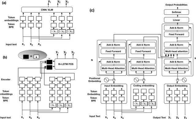
3 Coding Combination

Below, we will discuss how to incorporate various types of codings in NLP tasks. Firstly, we code each word independently. Then, the word embed-ding (Mikolov et al.,2013) is trained on code- and word-based sentences separately. After that, we treat this new form of sentence representation and its written text form as two source inputs to the encoder and feed their combination into a baseline NN-NLP system. Thus, our coding is realized as a portable module that provides inputs to any NN architecture. We introduce three different combi-nation methods to implement the interface of our coding module to various NN architectures.

We implement the combination of the text and the code forms in three ways: (1) concatenation

(see Figure3a); (2) linear interpolation (see

Fig-ure3b), where the dark color boxes have the

op-eration of “+”; (3) multi-source encoding on

Bi-LSTM (see Figure3b), as well as on Transformer

(see Figure3c). It is worth noting that there is no additional data or information needed except for our coding algorithms themselves.

3.1 Concatenation

Applying a coding function in Equation1on each

word x1, x2, x3,· · ·, xi,· · ·, xI0 in an input

sen-tence one-by-one generates a sequence of code-words γ(x1), γ(x2), γ(x3),· · ·, γ(xi),· · ·, γ(xI0)

in the same lengthI0. Note that we use the term

“word” loosely here, which can mean a word or a subword, or even a character.

The first combination method is concatenating

two input sources. We apply the

x₁ x₂ x₃ Input text Token BPE Token embeddings CNN/ XLM y1 y2 y3 (a) c₁ c₂ c₃ x₁ x₂ x₃ Input text Token BPE Token embeddings c1 c2 c3 Bi-LSTM POS y1 y2 y3 + + Encoder (b) linear combination + = + x₁ x₂ x₃ Input Text Token BPE Token Embedding

Input Embedding Coding embedding

Add & Norm Multi-Head Attention

Positional Embedding

N

Add & Norm Feed Forward

Add & Norm Multi-Head Attention

Add & Norm Feed Forward

y₁ y₂ y₃

Output Text

Output Embedding Add & Norm Multi-Head Attention

Add & Norm Multi-head attention

Add & Norm Feed Forward Softmax Linear Output Probabilities N + + + (c) c₁ c₂ c₃

Figure 3: Combination methods for different NN architectures: (a) concatenation for ConvS2S and XLM; (b) linear interpolation and multi-source encoding for Bi-LSTM with attention; (c) multi-source encoding for Transformer.

word embeddings implemented by Reh˚uˇrekˇ

and Sojka (2010) on each word (x) and its

codeword γ(γ(x)). We separately train word

embedding on code- and textual sentences.

Thus, γ(·) and (·) are different functions.

As shown in Figure 3a, the input to the NLP

system is the embedded words of a sentence,

˜

(x1),˜(x2),˜(x3),· · ·,˜(xi),· · ·,˜(xI), where

˜

(xi)is the concatenation of the embedded word

(xi)and its codewordγ(γ(xi)):

˜

(xi) = [(xi);γ(γ(xi))] (2)

3.2 Linear Combination

The concatenation method merges two input sources and train one encoder for both. How-ever, it may be beneficial to have textual and codeword embeddings and encoders trained sep-arately, because they have different vocabularies. Then, those two encoders are combined linearly, a widely applied model combination technique. The input to the linear combiner is the encoded sentence, represented by a sequence of hidden statesh˜1_((x

I)),· · ·,h˜j((xI)),· · ·,h˜J((xI))of

the last position I in each of the encoder layer

j∈[1,2,· · ·, J]. Jis the number of nodes at each decoder layer. Recall that each hidden state is a

real vectorRd, and that is why we can use the

vec-tor space operations such as addition on it. For convenience, we denote the last hidden state of the j-th encoder layer that we take as the input to the decoder,h˜j_((x

I)), by˜hj_I, the last hidden state of

thej-th encoder layer of the original textual sen-tencehj((xI))byhj_I, and the last hidden state of

thej-th encoder layer of the code-based sentence hj(γ(γ(xI)))byhγjI. The combined encoder

hid-den stateh˜j is a linear interpolation of the hidden states of the textural input and its codeword input:

˜

hj = (1−α)hj_I+αhγjI (3)

As shown in Figure (3b), the combined last

hid-den state in each layer is fed into the baseline de-coder. The black blocks contains only the operator of+, as shown in the gray ellipse.αis the encoder weight of the coded sentence, and here,α= 0.5.

3.3 Multi-Source Encoding.

In the linear combination method, the weight α

is shared among all states in one encoder. To al-low different weights for each state, we implement

variations of multi-source encoding by Zoph and

Knight(2016) for the POS tagging model (Joshi,

2018) (see Figure3b). The combined hidden state

˜

concatenation of word-based and code-based hid-den states of the last positionIin layerjmultiplied

by the weightWc

˜

hj = tanh(Wc[h_Ij;hγj_I]). (4)

Bi-LSTM In Bi-LSTM decoder, the cell statec of an encoder is a concatenation of the forward and

backward cell states. The combined cell statec˜

is the sum of the word-basedcand code-basedcγ

encoder’s cell states

˜

c=c+cγ. (5)

Single-head Attention The attention model looks at both word-based and code-based encoders simultaneously. A context vector from each source encoderctandcγtis created instead of the justct

in the single-source attention model. Hidden states from the top decoder layer looks back at previous hidden statesht˜−1 and the context vectors of the

encoders:

˜

ht= tanh(Wc[ ˜ht−1;ct;cγt]) (6)

Multi-head Attention Multi-head attention al-lows the model to jointly attend to information from different representation subspaces at

differ-ent positions. We apply the Fairseq (Ott et al.,

2019) implementation of Multilingual Translation

in Transformer (Vaswani et al.,2017) treating text and codewords as two language inputs. The multi-lingual transformer trains on two encoders in turn iteratively. For example, in the first epoch it trains the textual encoder then trains the codeword en-coder; in the second epoch, it trains again the tex-tual then the codeword encoder, and so on.

4 NLP Applications

4.1 Combination Methods

NMT We improve over two state-of-the-art

Neu-ral Machine Translation (NMT) baselines: the Convolutional Sequence to Sequence Learning

(ConvS2S) byGehring et al.(2017) and the

Trans-former byVaswani et al.(2017). On ConvS2S, we

concatenate (+) the input sentence with its coded

sentence using the method in §3.1illustrated in

Figure3a. On the Transformer baseline, we

com-bine the input sentence with the encoded sentence

using “multi-head attention” as described in§3.3

and illustrated in Figure3c.

LM For Neural Language Modeling, we treat the

text sentence as one language and the coded sen-tence as another language and combine them with

the cross-lingual Language model (XLM;Lample

and Conneau,2019) using the toolkit introduced

inOtt et al.(2019). The combination method is in

§3.1and Figure3a.

POS tagging We implement linear combination illustrated in Figure3b (with the gray area) and non-linear multi-encoders that are described in Equa-tions (4) to (6) and Figure 3b (without the gray area). The input to the multi-encoder is the text and coded sentences, and its output is directly fed into the POS tagger. For the linear combined en-coder, we element-wise linearly interpolate the text encoding vector and the code coding vector, each trained separately. For example, the subscript “0.5” indicates an interpolation with equal weights.

4.2 Application 1: Machine Translation Tasks and Languages. We verify our

ap-proaches on three MT tasks (datasets):

WMT’14 (WMT, 2014), WMT’18 (WMT,

2018), and IWSLT’17 (IWSLT,2017)). We carry

out experiments for different translation directions: English to French (EN-FR), French to English (FR-EN), English to German (EN-DE), German to English (DE-EN), and Chinese to English (ZH-EN). EN DE EN FR Raw Sents. 4.59 2.81 Pre-processed Sents. 4.03 2.48 Before BPE R.W. 102 98 67 58 After BPE R.W. 54 56 68 60

Table 1: Number of Sentences (Sents.) and Running Word (R.W.) as well as Vocabulary size (Voc.) [M] of WMT’14 News (EN-DE) and WMT’18 Bio (EN-FR)

Before BPE After BPE Task WMT’14 WMT’18 WMT’14 WMT’18 Coding EN DE FR EN EN DE FR EN Baseline 711 1500 366 338 33 35 29 24 +Soundex 717 1500 - - 33 33 - -+Metaphone 904 1500 480 338 34 30 30 21 +NYSIIS 981 1500 523 338 34 30 30 20 +EL9 1400 1500 732 338 34 25 30 18 +Huffman9 1400 1500 732 338 34 25 30 16

Table 2: Vocabulary size [K] of WMT’14 News (EN-DE) and WMT’18 Bio (EN-FR) before and after applying BPE with different codings.

WMT’14 and WMT’18 We conduct experi-ments on WMT’14 News English-German dataset,

which contains around 4.6 million sentences

Figure 4: Translation results in BLEU[%] on WMT’14 News and WMT’18 Bio task. BPE operations: 32k. Baseline is (Gehring et al.,2017) on words. In this pa-per, we denote baselines for all experiments on all tasks with their names, referring to standard textual word in-puts. Systems by adding the codeword inputs on base-lines are denoted as “+..”.

on English-French dataset forn WMT’18

Biomed-ical Task that contains around 2.8 million

sen-tences. Table1shows vocabulary statistics on the

source/target of the training data before and after applying codings. We use Moses tokenizer and restrict 250 characters per sentence and 1.5 length ratio between source and target sentences as a filter in pre-processing. The Byte-pair encoding model is jointly trained on the source textual word inputs, codeword inputs, and target outputs for French and German systems, and separately trained on the source and target for Chinese systems. We applied concatenation for ConvS2S baselines and multi-source encoding for transformer baselines in all tasks, respectively. For ConvS2S we set the em-bedding dimension as 512, the learning rate as 0.25, the gradient clipping as 0.1, the dropout ratio as 0.2, and the optimizer as NAG. For transformer, we set the embedding dimension as 512, the learning rate as 0.0005, the minimum learning rate as10−9_{, the}

warmup learning rate as10−7, the optimizer batas as 0.9 and 0.98 for adam optimizer, the dropout ratio as 0.3, the weight decay as 0.0001, the shared decoders and shared decoder embedding as true. The training is terminated until the validation loss does not decrease for five consecutive epochs. We

compute the BLEU score usingsacrebleu.

As shown in Figure4, on WMT’18 we achieve

an improvement of +0.7 BLEU points for English-German and +0.8 BLEU points for French-English, respectively. Some phonetic coding may be more suitable for certain languages than others. Meta-phone works best for English because it handles spelling variations and inconsistencies. According to its orthography, the German spelling is largely

phonetic (unlike English spelling), thus adding pho-netics does not help much in DE-EN NMT.

Figure 5: Translation results in BLEU[%] on small task IWSLT’17. FR-EN & EN-FR. BPE:16k. Baseline is (Vaswani et al.,2017) on words. Dev: test2013-2015; Test: test2017.

Figure 6: Translation results in BLEU[%] on small task IWSLT’17. ZH-EN. BPE:16k. Baselines are (Gehring et al., 2017; Vaswani et al., 2017) on words. Dev: test2010-2015; Test: test2017.

Figure 7: Translation results in BLEU[%] on small task IWSLT’17. DE-EN, EN-DE. BPE:16k. Baselines are (Gehring et al.,2017) on words. Dev: test2010-2015; Test: test2017.

IWSLT In IWSLT’17 task, we achieved +5.2 BLEU point on EN-FR and +1.9 BLEU point on FR-EN. We also add Pinyin for Chinese-English

translation on IWSLT’17 (IWSLT,2017) as a

sup-plementary experiment. Adding Wubi also en-hances the baseline performance. On the Trans-former baseline, we use the codewords as the input source test set during decoding. Note that all exper-iments are conducted on the real datasets, without using/verifying on any artificial noise anywhere.

Model Complexity. We tune the dropout param-eters for conducting the following experiments:

WordsandW+Metaphoneon IWSLT’17 EN-FR. The drop out value is set by default to 0.2, and

the beam-size to 12. Figure8shows how

transla-tion accuracy changes by varying the dropout value. The highest BLEU score is at a dropout of 0.2 for the baseline and 0.2 and 0.3 in our approach. A higher optimal value of dropout means fewer nodes in the Neural Networks are needed to opt NMT quality. This implies that adding auxiliary inputs will reduce the model complexity.

Figure 8: Dropout optimum. x-axis: the dropout value.

Model parameter size. Table 3 shows the change of the parameter size when applying our approaches. Our parameters include weights and biases of neural network models. The parameter size reduces when we concatenate the original in-puts with our codewords because the vocabulary size reduces (although the BPE operations stay the same as the baseline). The parameter size increases when we use the multi-source encoding because we added more encoder for the codeword input.

Baseline ConvS2S Transformer WMT WMT IWSLT IWSLT ’14 ’18 ’17 ’17 SRC EN FR EN DE EN FR TGT DE EN DE EN FR EN Baseline 198 181 14 13 57 57 +Soundex 196 - 13 12 77 77 +NYSIIS 193 177 12 11 78 -+Metaphone 193 178 12 11 77 77 +EL9 187 174 12 11 75 75 +Huffman9 187 173 12 11 75 75

Table 3: Number of model parameters [M] on WMT’14 News, WMT’18 Bio, and IWSLT’17 tasks. Baselines are ConvS2S and Transformer on word input. Systems by adding the codeword inputs on baselines are denoted as “+..”.

Training Speed. Table5shows the system

train-ing time (with BPE32koperations). The total time

(in minutes) is listed in the first column, and the number of epochs is in the second. Combining codewords reduces the model complexity. There-fore, the training becomes more efficient and needs

ZH-EN ZH-EN ConvS2S 14 Transformer 59 +Pinyin 18 +Pinyin 78 +Wubi 18 +Wubi 78 +EL9 18 +EL9 77 +Huffman9 18 +Huffman9 77

Table 4: Number of model parameters [M] on IWSLT’17 Chinese-English task. Baselines are (Gehring et al.,2017) and (Vaswani et al.,2017) on words. Systems by adding the codeword inputs on baselines are denoted as “+..”.

a smaller number of epochs to converge. The total training time of our approaches is comparable to that of baselines, sometimes even less.

EN-DE FR-EN ConvS2S 166/24 93/16 +Soundex 241/26 -+NYSIIS 266/33 147/15 +Metaphone 233/21 143/15 +EL9 249/26 145/12 +Huffman9 245/25 151/15

Table 5: Training time (in minutes) per epoch/ epoch number.

Output example. Table6shows a translation ex-ample. Combining phonetic coding helps to in-clude more subwords that cannot be obtained from text.

Source The firefighters were brilliant. Reference Die Feuerwehrleute waren großartig.

ConvS2S Die Feuerwehr war brillant.

+MetaPhone Die Feuerwehrleute waren brilliant . Table 6: An MT WMT’14 EN-DE output example: +Meta-Phone coding generates new subwords “fire” and “fighter” that improves the translation over the baseline ConvS2S.

4.3 Application 2: Language Modeling (LM) Task and result. We train and evaluate the En-glish part of EN-FR IWSLT’17 dataset and also on English part of EN-DE WMT’14 News dataset. We use 256 embedding dimensions, six layers, and eight heads for efficiency. We set dropouts to 0.1, the learning rate to 0.0001, and BPE operations to

32k. We used Adam optimizer with betas of 0.9

0.999. As shown in Table7, adding Metaphone

sig-nificantly reduces PPL of the baseline system, i.e., 20.1% relatively. “+NYSIIS WA” indicates the system with NYSIIS but adding word alignments

between English and its coded form; see Table7.

4.4 Application 3: POS Tagging

Task and result We evaluate our approach

in POS Tagging on Brown Corpus (Francis and

WMT’14 IWSLT’17 Dev Test Dev Test XLM 1.17 1.18 28.04 26.07 +NYSIIS 1.17 1.18 24.00 22.64 +Metaphone 1.17 1.18 23.55 20.8 (-20.1%) +Soundex 1.17 1.18 23.60 22.20 +NYSIIS WA 1.14 1.15 23.50 21.64 +Metaphone WA 1.14 1.15 (-2.4%) 23.49 20.94

Table 7: LM PPL improvements on the English part of a subset of WMT’14 News EN-DE and IWSLT’17 EN-FR.

English dataset for POS and contains 57 341 sam-ples. We uniform randomly sample 64% data as the training set, 16% as the validation set, and 20% as the test set. Our baseline is a Keras (Chollet,

2015) implementation (Joshi,2018) of Bi-LSTM

POS Tagger (Wang et al.,2015). We train word

embedding (Mikolov et al., 2013) implemented

byReh˚uˇrek and Sojkaˇ (2010) with 100 dimensions.

Each of the forward and the backward LSTM has 64 dimensions. We use a categorical cross-entropy loss and RMSProp optimizer. We also use early

stopping based on validation loss. As in Table8,

the linear multi-encoder withα = 0.9brings the

best results, i.e. -15.79% relative improvement over the baseline.

Dev Test

Loss Accuracy Error Rate Berkeley Parser 5.24 5.08 98.67 1.33 +MetaPhone0.5 4.90 4.72 98.72 1.28 (-3.76%)

+MetaPhone0.9 4.05 4.29 98.87 1.13 (-15.04%)

+NYSIIS0.9 4.16 4.38 98.88 1.12 (-15.79%)

Table 8: POS with phonetic codings Brown corpus.

5 Related Work

Previous important work investigated the role of auxiliary information to NLP tasks, such as

poly-semous word embedding structures byArora et al.

(2016), factored models byGarc´ıa-Mart´ınez et al.

(2016), and feature compilation bySennrich and

Haddow(2016). We emphasize that we do not use

any additional information besides our algorithms.

Hayes(1996);Johnson et al.(2015) applied

ex-plicit phonological rules or constraints to tasks such as word segmentation. In neural networks, we can implicitly learn from phonetic data and leave the networks to discover hidden phonetic features through end-to-end training opt specific NLP tasks, instead of applying hand-coded constraints.

Closely related, but independent to our work, is

the character-based MT, such as the work ofLing

et al.(2015) andChung et al.(2016), among many

others. We go beyond text level representations and look for novel representations for decompositions, sometimes even smaller than characters.

Different from the inspiring work that

uses Pinyin (Du and Way, 2017), skip-ngram

(Bojanowski et al., 2017), and Huffman on

source/target (Chitnis and DeNero, 2015), our

study aims to improve NN-NLP including NMT overall rather than only eliminating unknown words, introducing six new codings into NLP in addition to Pinyin and text. Importantly, our artificial codings apply on all languages. Moreover, we achieve experimental improvements overall.

Liu et al. (2018) added Pinyin embedding to

robustify NMT against homophone noises. They described that it was unknown why Pinyin also im-proved predictions on the clean test. This is a very interesting work, and we explain this phenomenon

through our theory thatthe multi-channel coding

offers an ensemble of the code words and the text, making the communication more reliable.

6 Conclusion

In this paper, we conduct a comprehensive study on how to code textual inputs from multiple linguistically-motivated perspectives and how to integrate alternative language representations into NN-NLP systems. We propose to use Soundex, NYSIIS, MetaPhone, logogram, fixed-output-length, and Huffman codings into NLP and de-scribe how to combine them in state-of-the-art NN architectures, such as Transformer, ConvS2S, Bi-LSTM with attentions. Our paradigm is general for any language and adaptable to various models. We conduct extensive experiments on five languages over six tasks. Our approach appears to be very use-ful and achieves up to 20.77%, 20%, and 15.79% relative improvements on state-of-the-art models of MT, LM, and POS, respectively.

Acknowledgement

We appreciate the National Science Foundation

(NSF) Award No. 1747728 and the National

Science Foundation of China (NSFC) Award No. 61672524 to fund this research. We also appreciate the JSALT workshop to support us in continuing this work. In particular, we thank all feedback pro-vided by the colleagues there. We also thank the comments of Periklis Papakonstantinou. Finally, we appreciate the support of the Google Cloud Re-search Program.

References

Sanjeev Arora, Yuanzhi Li, Yingyu Liang, Tengyu Ma, and Andrej Risteski. 2016. Linear Algebraic struc-ture of word senses, with Applications to Polysemy. Transactions of the Association for Computational Linguistics.

Piotr Bojanowski, Edouard Grave, Armand Joulin, and Tomas Mikolov. 2017. Enriching word vectors with subword information. Transactions of the Associa-tion for ComputaAssocia-tional Linguistics.

Rohan Chitnis and John DeNero. 2015. Variable-length word encodings for neural translation models. InProceedings of the 2015 Conference on Empirical Methods in Natural Language Processing.

Franc¸ois Chollet. 2015. Keras. https://github. com/keras-team/keras.git.

Junyoung Chung, Kyunghyun Cho, and Yoshua Ben-gio. 2016. A character-level decoder without ex-plicit segmentation for neural machine translation. In Proceedings of Association for Computational Linguistics.

Jinhua Du and Andy Way. 2017. Pinyin as subword unit for Chinese-sourced neural machine translation. In Proceedings of Irish Conference on Artificial In-telligence and Cognitive Science.

W. N. Francis and H. Kucera. 1979. Brown corpus manual. Technical report, Department of Linguis-tics, Brown University, Providence, Rhode Island, US.

Mercedes Garc´ıa-Mart´ınez, Lo¨ıc Barrault, and Fethi Bougares. 2016. Factored neural machine transla-tion. Computing Research Repository.

Jonas Gehring, Michael Auli, David Grangier, Denis Yarats, and Yann N. Dauphin. 2017. Convolutional sequence to sequence learning. In Proceedings of International Conference on Machine Learning. Bruce Hayes. 1996. Phonetically driven phonology:

The role of optimality theory and inductive ground-ing. rutgers optimality archive. In Proceedings of Conference on Formalism and Functionalism in Lin-guistics.

David A Huffman. 1952. A method for the construc-tion of minimum-redundancy codes. Proceedings of the Institute of Radio Engineers.

IWSLT. 2017. Homepage of International Work-shop on Spoken Language Translation 2017. http://workshop2017.iwslt.org/.

Mark Johnson, Joe Pater, Robert Staubs, and Em-manuel Dupoux. 2015. Sign constraints on feature weights improve a joint model of word segmentation and phonology. InProceedings of North American Chapter of the Association for Computational Lin-guistics: Human Language Technologies.

Aneesh Joshi. 2018. LSTM POS tagger.

https://github.com/aneesh-joshi/LSTM_ POS_Tagger.git.

Guillaume Lample and Alexis Conneau. 2019. Cross-lingual language model pretraining. Advances in Neural Information Processing Systems.

Wang Ling, Isabel Trancoso, Chris Dyer, and Alan W Black. 2015. Character-based neural machine trans-lation. Proceedings of the 54th Annual Meeting of the Association for Computational Linguistics -Short Papers.

Hairong Liu, Mingbo Ma, Liang Huang, Hao Xiong, and Zhongjun He. 2018. Robust neural machine translation with joint textual and phonetic embed-ding. InProceedings of Association for Computa-tional Linguistics.

Tomas Mikolov, Ilya Sutskever, Kai Chen, Greg S Cor-rado, and Jeff Dean. 2013. Distributed representa-tions of words and phrases and their composition-ality. In C. J. C. Burges, L. Bottou, M. Welling, Z. Ghahramani, and K. Q. Weinberger, editors, Ad-vances in Neural Information Processing Systems. Curran Associates, Inc.

Myle Ott, Sergey Edunov, Alexei Baevski, Angela Fan, Sam Gross, Nathan Ng, David Grangier, and Michael Auli. 2019. fairseq: A fast, extensible toolkit for sequence modeling. In Proceedings of North American Chapter of the Association for Com-putational Linguistics: Human Language Technolo-gies.

Lawrence Philips. 1990. Hanging on the metaphone. Computer Language.

P Rajkovic and D Jankovic. 2007. Adaptation and ap-plication of daitch-mokotoff Soundex algorithm on serbian names. InProceedings of Conference on Ap-plied Mathematics.

Radim ˇReh˚uˇrek and Petr Sojka. 2010. Software Frame-work for Topic Modelling with Large Corpora. In Proceedings of the Conference on Language Re-sources and Evaluation 2010 Workshop on New Challenges for NLP Frameworks, pages 45–50, Val-letta, Malta. ELRA.

Robert C. Russel. 1918. A method of phonetic index-ing.Patent no. 1,261,167.

Ferdinand de Saussure. 1916. Course in General Lin-guistics. Duckworth, London. (trans. Roy Harris). ISBN 9780231527958, 0231527950.

Rico Sennrich and Barry Haddow. 2016. Linguistic in-put features improve neural machine translation. In Proceedings of Conference on Machine Translation. Rico Sennrich, Barry Haddow, and Alexandra Birch. 2015. Neural machine translation of rare words with subword units.Proceedings of the 54th Annual Meeting of the Association for Computational Lin-guistics.

Ashish Vaswani, Noam Shazeer, Niki Parmar, Jakob Uszkoreit, Llion Jones, Aidan N Gomez, Ł ukasz Kaiser, and Illia Polosukhin. 2017. Attention is all you need. InAdvances in Neural Information Pro-cessing Systems.

Peilu Wang, Yao Qian, Frank K. Soong, Lei He, and Hai Zhao. 2015. Part-of-speech tagging with bidi-rectional long short-term memory recurrent neural network.Computing Research Repository.

WMT. 2014. Homepage of Workshop on Statistical Machine Translation 2014. http://www.statmt.org/wmt14/.

WMT. 2018. Homepage of Workshop on Sta-tistical Machine Translation 2018: Biomedical task. http://www.statmt.org/wmt18/biomedical-translation-task.html.

George Zipf. 1935. The Psychobiology of Language: An Introduction to Dynamic Philology. M.I.T. Press, Cambridge, Mass.

Barret Zoph and Kevin Knight. 2016. Multi-source neural translation. In Proceedings of North Amer-ican Chapter of the Association for Computational Linguistics: Human Language Technologies.