Neural-Learning-Based Force Sensorless
Admittance Control for Robots with Input Deadzone
Guangzhu Peng, C. L. Philip Chen,
Fellow, IEEE
, Wei He,
Senior Member, IEEE
,
and Chenguang Yang,
Senior Member, IEEE
Abstract—This paper presents a neural networks based admit-tance control scheme for robotic manipulators when interacting with the unknown environment in the presence of the actuator deadzone without needing force sensing. A compliant behaviour of robotic manipulators in response to external torques from the unknown environment is achieved by admittance control. In-spired by broad learning system (BLS), a flatted neural network structure using Radial Basis Function (RBF) with incremental learning algorithm is proposed to estimate the external torque, which can avoid retraining process if the system is modelled insufficiently. To deal with uncertainties in the robot system, an adaptive neural controller with dynamic learning framework is developed to ensure the tracking performance. Experiments on the Baxter robot have been implemented to test the effectiveness of the proposed method.
Index Terms—neural networks (NNs); adaptive control; broad learning; force/torque observer; admittance control.
I. INTRODUCTION
I
Nthe past decades, robots have been widely applied in many fields of social life, such as industry, service and education [1]. In these cases, robots are inevitably encountering the un-known environment. Therefore, control of robots in a safe and compliant behaviour during the interactive process has been widely studied. In the literature, hybrid position/force control and impedance control have been the two main approaches for interaction control [2]–[5].Impedance control aims to impose a desired dynamic be-havior on the robot to interact with environments. The desired interaction performance is specified through a impedance model. On the basis of the control causality, admittance control could be regarded as the inverse of impedance control [6]. The admittance control can ensure the robot produce a good interaction performance by adapting the motion to the external force. The admittance control aims to map the
This work was partially supported by Engineering and Physical Sciences Research Council (EPSRC) under Grant EP/S001913, National Natural Sci-ence Foundation of China under Grant 61751202, Grant 61751205, Grant U1813203, and Grant U1801262, in part by the Science and Technology De-velopment Fund, Macau SAR (File no. 079/2017/A2, and 0119/2018/A3), in
part by the Multiyear Research Grants of University of Macau.Corresponding
author: C. L. Philip Chen.
G. Peng is with the Department of Computer and Information Science, Faculty of Science and Technology, University of Macau, Macau 999078, China (Email: [email protected]).
C. L. Philip Chen is with School of Computer Science and Engineering, South China University of Technology, Guangzhou 510641, China, with the Unmanned System Research Institute, Northwestern Polytechnical University, XiAn, 710072, China, and also with the Faculty of Science and Technology, University of Macau, Macau 999078, China (e-mail: [email protected]).
W. He is with Institute of Artificial Intelligence, University of Science and Technology Beijing, Beijing 100083, China, and also with School of Automation and Electrical Engineering, University of Science and Technology Beijing, Beijing 100083, China (Email:[email protected]).
C. Yang is with Bristol Robotics Laboratory, University of the West of England, Bristol, BS16 1QY, UK (Email: [email protected]).
external force measured by the force sensors to the position of the robot end-effector through an admittance model. In general admittance control schemes, the inner-loop is for trajectory tracking, which accepts the trajectory generated by the admittance model in the out-loop as the input signal [7]. In addition, the admittance model varies from different tasks. This characteristic enables the admittance control to be used in many forms to achieve a good physical interaction control performance [8].
In admittance control schemes, force measurement is funda-mental and necessary, and the interactive control performance is largely decided by the accuracy of the external force measurement [9]. A common method is to use force sensors to measure external forces. Although the force sensor can provide high precision, it also has shortcomings. First of all, commercial sensors with high precision are often expensive. Secondly, force sensors mounted on robots will change the dynamics of robots [10]. Finally, due to exposure to the com-plex and dangerous industrial environment, the force sensor will be vulnerable to damage, which is not applicable to certain situations. Therefore, force observer approaches have been widely studied. In [11] [12], the disturbance observer approach was proposed to estimate the external force. In [13], a dynamic state observer was proposed to estimate the contact force. In [14], generalized momentum based observer was used for measuring the contact force with partially known model dynamics. These classical model-based observer methods can not work well without accurate model dynamics.
To solve this problem, many force estimation methods integrating neural networks have been studied [15] [16]. In [15], a NN-improved disturbance observer was proposed with partial dynamics of the robotic link. In [16], NNs were em-ployed to approximate the Coulomb friction and improve the performance of the model-based observer. Although NNs were employed into the above methods, the problem of requiring system dynamics is still unsolved. In [17], an inverse dynamics method combining with multilayer feedforward NNs have been proposed without robot dynamic model. NNs were used to identify the system dynamics and have a good approxima-tion performance. However, this architecture will consumes more time as the number of layers of neural network increases. Compared with traditional multilayer NNs, the random vec-tor functional-link neural network (RVFLNN) is an effective network with good approximation ability and simple structure. Moreover, it can avoid long training time and has fast learning property [18] [19]. Considering this good property, the inverse dynamics observer combined with RVFLNN is proposed for external force. The advantage is that the dynamics of robot system is not required and the training time of the NN structure is shorter.
practical control system [20]. In the literature, adaptive con-trol methods incorporating intelligent tools have been widely employed in control systems [21]–[24]. Different from model-based control approaches, these adaptive control methods could deal with the unknown system dynamics by automat-ically updating laws. Although model-based control usually shows better control performance, it is based on an accurate model [25]. In practice, an accurate model is hardly to be obtained owing to the complexity of mechanical robot system. In addition, the payload on the manipulator could also make the modelling of the robotic arm more difficult [26]. In [27], the RBFNN was employed to deal with uncertainties of both robot system and the object, and a prescribed tracking performance was guaranteed. In [28], NNs were integrated in control design to cope with the uncertain dynamics. In [29], the adaptive fuzzy control method was used to suppress the uncertain dynamics of the system. Although NNs or fuzzy logic can solve the problem of system uncertainties, these intelligent tools inevitably increase the burden of control system. In order to have good approximation performance, the number of neurons and fuzzy rules will increase, which in turn will bring heavy computation burden to the system and affect the control effect. Moreover, when the learning is insufficient, the inaccurate approximation will influence the control performance. However, among the literatures about adaptive NN control, few studies have concerned with the the way of solving the problems of the insufficient learning condition and computational burden.
Recently, the broad learning system (BLS) has attracted much attention because of its novel framework without suf-fering time-consuming training process caused by traditional deep structure, and it has been used in pattern recognition and classification [30] [31]. Considering its novel architechture, the property of BLS could also be employed to NN based control scheme to accumulate the learning experience with node expansion without retraining the model. In [32], it has been pointed out that deterministic learning theory is an efficient way to deal with the unknown dynamics by satisfying the persistent excitation (PE) condition. Based on the above discussion, an adaptive RBFNN learning framework has been developed. Compared with the traditional learning network, the difference is that this adaptive learning framework can not only ensure the approximation ability of NNs under insufficient learning condition, but also will not bring heavy computational burden to the system.
Deadzone is an crucial problem of affecting the dynamic control performance of the system. In practical systems, the deadzone will not only cause the loss of control precision, but also cause system instability. Researchers have proposed many methods to solve this problem. In [33], an adaptive method was incorporated into motion control system for tuning fuzzy logic parameters. In [34], the deadzone nonlinearities in control system were compensated by inverse function. However, due to the complexity and uncertainties of practi-cal actuators, the deadzone functions are difficult to know. Therefore, such model-based compensation methods may not have good performance in practical systems. With the strong approximation ability, NNs have been applied into control system to compensate the deadzone nonlinearity [35]–[38]. Inspired by above works, in this paper, a NN-based force sensorless admittance control scheme for robotic arms with actuator deadzone is proposed. This paper is a continuation of
our previous work [39], and the improvements are given as follows:
(i) Admittance control is adopted to generate a compliant interactive behaviour with considering the dynamics of the unknown environment. A saturation function in joint space is considered to constraint the robot motion.
(ii) A flatted neural network structure using RBF with incremental learning is proposed to estimate the external torque rather than model-based observer.
(iii) A RBFNN-based learning controller with dynamic framework is developed to deal with system uncertainties and compensate the deadzone nonlinearities.
The rest of this paper is organized as follow. Section II expresses the preliminaries. Control design is presented in Section III. Section IV gives the experimental results. Conclusion is drawn in Section V, and appendix is presented in section VI.
II. PRELIMINARIES
A. Problem Formulation
The dynamics of a n−link robotic manipulator is
Mq(q)¨q+Cq(q,q˙) ˙q+Gq(q) =τ+JTfext (1)
where q¨∈ Rn,q˙ ∈
Rn andq ∈Rn represent joint accelera-tion, velocity and posiaccelera-tion, respectively. Mq(q)∈ Rn×n and
Cq(q,q˙)∈Rn×n denote the inertia and coriolis matrices, and
Gq(q) ∈ Rn is the gravity load. τ ∈ Rn is the joint torque and fext is the external force. The relationship between the
external torque and the force can be written as
τext=JTfext (2)
whereJ(q)is the manipulator Jacobian matrix.
Property 1: The matrix Mq(q) is symmetric and positive definite [40].
Property 2: The matrix 2Cq(q,q˙) − M˙q(q) is
skew-symmetric [40].
The environmental dynamics can be defined as
MEx¨+CEx˙ +GEx=−fext (3)
where ME, CE and GE are the coefficient matrices. x¨, x˙
and x denote the acceleration, velocity and position of the end-effector of the manipulator, respectively. Through inverse kinematics and (2), the environmental dynamics in (3) can be transformed to joint space to describe the environment dynamics, such that
Φ( ˙q, q) =τext (4)
whereΦ(·)denotes the mapping function.
In this paper, a damping-stiffness admittance model [41] is used to describe this relationship, such as
Cd( ˙xr−xd˙ ) +Gd(xr−xd) =−fext (5)
where xd andxr denote the desired trajectory and modified
desired trajectory in task space, respectively. Cd andGd are coefficient matrices. According to (5), compliant motionxrfor the external force is generated based on the desired trajectory
xd andfext. In joint space, the admittance model (5) can be
described as
Fig. 1. The structure and updating algorithm for Functional-link neural network (modified from [19]).
whereϕ(·) denotes the robot kinematics function,qr and qd
denote the modified desired trajectory and desired trajectory in joint space, respectively.
In admittance control schemes, the modified desired tra-jectory qr is always assumed to be bounded, i.e., |qri| < Ci, (i= 1,2...n), where Ci is a positive constant. However, during the process of robot-environment interaction, the mod-ified trajectory qr may violate the prescribed bound, that is,
|qri|> Ci, i= 1,2...n. To solve this problem, a saturation
function is defined as qri= −γi(1−e qri+ρiCi γi )−ρiCi, qri <−ρiCi
qri, |qri| ≤ρiCi
γi(1−eρiCi
−qri
γi ) +ρiCi, qri > ρiCi
(7)
whereγi = (1−ρi)Ci, 0 < ρi <1 (i = 1,2, .., n). Under this saturation function, the modified desired trajectoryqrcan be guaranteed to stay within a constraint space.
B. RBFNN with PE Property
In this part, a brief introduction of RBFNN approximation is given. In [42], it is proven that the RBFNN can approximate any continuous function f(•) with a sufficient large node l, and optimal weight W∗, that is
f(Zin) =W∗TS(Zin) +ε(Zin), ∀Zin∈ΩZin (8)
whereZin∈ΩZin ⊂R
υ is the input vector of RBFNN with
input dimensionυ.||ε(Zin)||< ε∗ denotes the approximation
error (|| • ||is the Euclidean norm of vectors).
It should be noticed that the activation function of RBFNN is Gaussian function
si(Zin) =exp[−(Zin−u
T
i )(Zin−ui)
η2
i
], i= 1, ..., l (9)
where l is the number of the NN node; ui =
[ui1, ui2, ..., uiυ] (i= 1,2, ..., l)andηidenotes the node center
and the variance, respectively.
In practice,W∗is the ideal NN weight matrix and estimated byWˆ, and the function can be approximated by
ˆ
f(Zin) = ˆW
T
S(Zin) (10)
where fˆ(Zin) is the estimate of f(Zin). The approximation error of the weight can be defined asW˜ = ˆW−W∗.
Definition 1: [32] Consider the lattice of RBFNN is con-structed in (8), we can select
%≥2h= min
i6=j ||ui−uj||>0 (11)
When the periodic input trajectoryZ0(t)is upon on the lattice, there will always be a regression subvector Sξ(Z
0
) in the
%−neighborhood ofZ0(t), such that
Sξ(Z0) = [s1(Z
0
1), ..., slξ(Z
0
lξ)] (12)
with different centers ui1, ..., uilξ. Because the value of the
regression vector becomes very small as the trajectory moves away from the centers, we can choose
2h≤%≤%0 (13)
with the distance betweenZ0 (i= 1,2, ..., lξ)and NN centers
satisfying||Zi0−uij||< %0, we can obtainsi(Z0)> %00, where
%00 is a small positive constant.
Lemma 1: [32]Assume that the periodic trajectoryZ0(t)is within a compact setΩ∈Rυ, and its derivative formZ˙0(t)is
bounded within Ω. If the centers of RBFNN could be placed on a sufficient large enough lattice to cover the compact setΩ, the Sξ(Z
0
)defined in (12) and (13) will satisfy the persistent excitation.
C. RVFLNN with Dynamic Updating Algorithm
The RVFLNN has a good ability of quick modeling for nonlinear systems with a simple structure, as shown in Fig. 1, whereξ(·)represents a mapping function for inputX, and
Wh,βh are randomly generated,Yn is the output matrix with
Yn=AnWn. In [19], an improvement version and a dynamic
updating algorithm for RVFLNN is proposed to calculate weights for new added enhancement nodes. The model is modified and illustrated in Fig. 1, where the pattern matrix
An:= [X|ξ(XWh+βh)]contains information of both input
and enhancement nodes, and a is a new enhancement node added into the network. In this part, the dynamic updating algorithm for calculating the weights based on the matrix pseudo-inverse will be introduced with an added enhancement node. First, we defineAp= [An|a], and the pseudoinverse of
the matrixAp is A+p = A+ n −dbT bT (14) whered=A+
na, andA+n denotes pseudoinverse of the matrix
An.
bT=
(
(I+dTd)dTA+n if c = 0
c+ if c6= 0 (15)
where c =a−And. Then, the weights Wn andWp can be computed by Wn = (λI+ATnAn)−1ATnYn Wp = Wn−dbTYn bTYn (16)
where Wn andWp denote the weights before and after new enhancement nodes are added into the network. As can be seen from the above equations, after adding new enhancement nodes, we only need to calculate the weight of the newly added
nodes and do not need to recalculate the weight of the whole network.
Remark 1: As presented in [30], it has been noted that there is no restriction on the the mapping feature functionξ(·)
from the input vector to the enhancement vector. In addition, this flatted neural network structure and the corresponding incremental learning algorithm can be applied in other neural network structures, such as support vector machine or RBF. Therefore, we choose the Gaussian function as the mapping function.
D. Actuator Deadzone
The deadzone nonlinearity is to describe the insensitivity of a system to small signals, as shown in Fig. 2.
Fig. 2. The deadzone nonlinearity (modified from [36]).
The deadzone nonlinearity can be described as [36]
D(τ) = gr(u−dr), τ ≥dr 0, dl< τ < dr gl(u−dl), τ ≤dl (17)
whereuis the actuator input;gr(·)andgl(·)are the unknown functions;dranddrare unknown parameters of the functions.
III. CONTROL DESIGN
A. Inverse Dynamics Method
In this section, a novel inverse-dynamics-based observer [17] with NNs is developed, and the revised architecture is shown in Fig. 3. The dynamics of the robotic arm in (1) can be Linearized as
τ+JTfext=Mq(q)¨q+Cq(q,q˙) ˙q+Gq(q)
= Ψ(¨q,q, q˙ )Π
=τf ree
(18)
whereτf reeis the torque to make the robotic arm move in free
motion. The right side of the (18) is parameterized. Ψis the regression matrix andΠis the parameter vector of the robotic arm. In this case, the estimation accuracy may be affected by inaccurate models or modelling errors. Traditional idea is to find a least squares solution ofΠ, and use it to estimate the contact forcefext, such that
ˆ
fext=J−T(Ψ(¨q,q, q˙ ) ˆΠ−τ)
=J−T(ˆτf ree−τ)
(19) whereΠˆ is estimate of the parameter vector. It is not difficult to find that the accuracy of the model directly affects the solution
Fig. 3. The NN-based observer under training (modified from [17]).
of the least squares. It is difficult to implement the inverse-dynamics-based observer if the robotic arm is not accurately modelled or the modelling error is relatively large.
To solve this problem, A flatted network structure with RBF is developed to estimate the model parameters. Compared with traditional multilayer feedforward neural networks employed in [17], this NN structure incorporating incremental learning algorithm can guarantee the approximation accuracy without remodelling the NN structure, when the approximation accu-racy is not satisfactory. As seen in (16), the advantage of incremental learning method is that the network only needs to train the weights of new added enhancement nodes without calculating the weights of the previous trained network. As depicted in Fig. 3, the inputs of the neural network under training are vectors of joint acceleration, velocity and joint position. After completing the training process, the trained NN model can be used to estimate the torqueτf ree and calculate
the external force from (19).
B. RBFNN Learning with Dynamic Framework
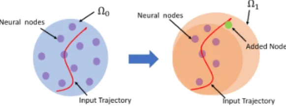
In this section, inspired the broad learning system, a dynam-ic RBFNN learning framework that combines node expansion and deterministic learning theory will be developed. As pre-sented in Fig. 4, the NN nodes with centers far away from the input trajectory will be discarded, and then the number of NN nodes will be decreased. Then newly added nodes with centers close to input trajectory will be properly placed, and the number of NN nodes will increase. Considering PE conditions and Lemma 1, the satisfied parameter estimation could not be achieved well when the input of RBFNN is far from the centers of the Guassian function, which will bring a low impact on the estimation performance. In this case, an extra NN node will be added to incorporate the new information. Here, the information of the added NN node is defined as [unew, ηnew, Wnew], where unew, ηnew, Wnew
denote the center, variance and the weight of the added NN node respectively. Suppose that the distance between centers of the nearest m NN nodes and the corresponding input is
dp= [p1, p2, ..., pm]. Then, the parameters of the added node
can be defined as
unew=p+γ||Zξ−p||
ηnew=ηi
(20) where Zξ is the current point of Zin, the initial weight of added NN node isWnew= 0,pdenotes the average distance
Fig. 4. The traditional RBFNN learning principle to enhancement of RBFNN learning (modified from [43]).
of dp, such as
p=
Pm
k=1pi
m , i= 1,2, ...m (21)
After that, centers vector of NN nodes can be rewritten as
ut+1=
[u
t, unew], if p >Ξ
ut, otherwise (22)
whereΞis the predefined threshold. After new enhancement nodes are added into networks, the weight vector can be rewritten as W(·n)= W(·) Wnew (23) whereW(·n)is the weight vector after new enhancement nodes
added into networks.
C. RBFNN Controller
In this part, a RBFNN-based controller is designed to guarantee the control performance. The tracking errors are defined as
e1=qr−q
α= ˙qr+K1e1
e2= ˙e1+K1e1
(24)
whereK1 = {k11, k12, ..., k1n} withk1i being positive
con-stant.
Considering the actuator deadzone, the robot dynamics (1) can be written as
Mq(q)¨q+Cq(q,q˙) ˙q+Gq(q) =D(τ) +τext (25)
whereD(·)is defined in (17). Design the control torque
τ = ˆMqα˙ + ˆCqα+ ˆGq+K2e2+ ∆ˆτ−ˆτext (26)
where∆ˆτ is the estimates of ∆τ = τ−D(τ), Mqˆ ,Cqˆ and
ˆ
Gq are the estimates of Mq, Cq andGq,ˆτext is the estimate
of τext;K2 is the control gain.
The updating law of RBFNN is
˙ˆ WM = Θ−M1(S(XM) ˙αe2−σMWˆM) ˙ˆ WC= Θ−C1(S(XC)αe2−σCWˆC) ˙ˆ WG= Θ−G1(S(XG)e2−σGWGˆ ) ˙ˆ Wτ =−Θ−τ1(S(Xτ)e2+στWτˆ ) (27)
where Θ(·) are positive definite matrices; σ(·) are positive
constants for disturbance [32].
Fig. 5. Description of the UUB and the definition in (38).
Substituting (26) into (25) yields
−Mqe˙2= ( ˆMq−Mq) ˙α+ ( ˆCq−Cq)α+ ( ˆGq−Gq)
+Cqe2−∆ˆτ+K2e2+ ∆τe
(28) where∆τe=τext−τextˆ .
Theorem 1: Considering the system dynamics (1), error signals (24), NN updating law (27) and Lyapunov function (32), the proposed control scheme can ensure thate2,||W˜(·)||
are UUB. Since||W∗
(·)||is bounded,||Wˆ(·)||=||W(∗·)+ ˜W(·)||
will be bounded. According to the definition in (24), we can obtain e1, α, qare bounded.
Remark 2: In [32], it has been proven that almost all periodic trajectories satisfy the (partial) PE condition. The approximation of uncertainties can be achieved with the lo-calized RBF neural networks (WˆTS(Zin)) when the tracking
convergence is obtained. In a possible large lattice on which the RBF neural network is constructed, the input trajectory could not search all the every neural node. Therefore, the NN learning will only occur in the localized area near the input trajectory of the neural network. For those neurons with centers close to the input trajectory, their weights can converge to a small neighborhoods of a set of the optimal weights. For those neurons far from the input trajectory, their weight will updates slightly, with little change. Since the centers are far from the input trajectory, the activation function S(Zin)
will be small and the weights remain small according to the updating law (27), which means little learning experience can be obtained. Therefore, we can present the restriction between the input orbit and centers to make the RBF neural network have the learned knowledge, that is
dis(qd, u)<Υ⇒ |WˆTS(Zin)−f(x)|< ε (29)
wheref(·)denotes the unknown function, andΥis a threshold specified by the designer. In this case, the unknown function is approximated by
f(x) =W∗TS(Zin) +ε(Zin)
= ˆWξTS(Zin) +ε0(Zin) (30)
where theWξˆ is the subvector ofWˆ, andε0 is the approxima-tion error.Wˆξ corresponds to the NN nodes with their centers
close to the input trajectory.
Considering that these neurons with centers far from the input orbit contribute little and bring extra computational burden to the system, in this paper, we will discard the NN nodes with centers far from the input trajectory according to the following principle
S(Zin)< λ, Zin∈Rυ (31)
Fig. 6. Illustration of the experimental setup.
IV. EXPERIMENT RESULTS
In this section, experiments are conducted to verify the effectiveness of our proposed method. The Baxter robot is a humanoid two-arm robot, each arm consists of seven joints: two shoulder joints s0, s1, two elbow joints e0, e1 and three
wrist joints w0, w1, w2. The model dynamic is introduced in
[44]. As shown in Fig. 6, the left arm of the Baxter robot is interacting with the external force form the environment, and the dynamics of the environment is modelled as the damping-stiffness system. The motion range of the robotic arm is specified within the constraint space.
A. Test of Adaptive RBFNN Controller
Firstly, the group of experiments aims to test the effec-tiveness of the RBFNN-based controller in the presence of actuator deadzone on joint s0. The upper and lower bounds
of the deadzone input are defined as dr = 0.49 and dl = −0.49. The RBFNNs are divided into two groups, one for approximating the unknown dynamics of robot system with
[q,q, α,˙ α, e˙ 2]∈R5n, the other for dealing with the problem
of input deazone, with [τ, q,q, e˙ 2] ∈ R4n. The center value
of Guassian function of neural networks nodes should be set within the range of the upper and lower bound of the robot motion and input limits, in [−1.5,1.5]×[−1.3,1.3]×
[−1.3,1.3]×[−1.3,1.3]×[−1,1]∪[−10,10]×[−1.3,1.3]×
[−1.5,1.5]×[−1,1]. The gains in updating law are selected as Θτ n =diag{0.125},ΘM =diag{0.3},ΘC=diag{0.3}, ΘG = diag{0.3}. The control parameters are selected as K1 = diag{12}, K2 = diag{6}. The desired trajectory is
specified asqd= [sin(5t);−1; 1.19; 1.94;−0.67; 1.03;−0.5].
The results are depicted in Figs. 7-12. As the input signal enters the deadzone space, the actuator could only provide little energy which cannot ensure the control performance, as shown in Fig. 10. In the Fig. 12, we can find that the deadzone condition (red solid line) is obvious at 10.5s and continued to 12.3s and difference between Dτ and control torqueτwill degrade the control performance as shown in Fig. 10. With the NN compensation, the tracking performance has been improved and the tracking error (red dotted line) with NN compensation is smaller than the controller (blue solid line) without compensation, as depicted in Figs. 9 and 11. Based on the forward kinematics of Baxter robot is given in [45], the tracking performance of end-effector with NN compensation is shown in Figs. 7-8. As shown in Fig. 7, the actual trajectory of the end-effector can follow the desired trajectory effectively, and the tracking error is less than0.04. As shown in Fig. 12,
0 0.1 0.05 1 0 0 -0.05 2 -0.1 -0.1 -0.15 actual desired
Fig. 7. The tracking performance of
the end-effector. -0.05 0.02 0.02 0 0 -0.02 0 0.05 -0.02 -0.04 -0.04 -0.06 error
Fig. 8. The tracking error of the end-effector. 0 5 10 15 20 25 30 t[s] -1.5 -1 -0.5 0 0.5 1 1.5 amplitude [rad] q1 qd1
Fig. 9. The tracking performance of
joints0with NN compensation.
0 5 10 15 20 25 30 t[s] -1.5 -1 -0.5 0 0.5 1 1.5 amplitude [rad] q1 qd1
Fig. 10. The tracking performance of
joints0 without NN compensation.
0 5 10 15 20 25 30 t[s] -0.2 -0.1 0 0.1 0.2 amplitude [rad]
tracking error without compensation tracking error with compensation
Fig. 11. The tracking errors of joint
s0with/without NN conpensation. 0 5 10 15 20 25 30 t[s] -10 -5 0 5 amptitude D 1 without compensation 1 with compensation 1
Fig. 12. The control inputs of joint
s0. 0 50 100 150 200 250 300 350 400 450 t[s] -5 0 5 magnitude [rad]
joint 1 joint 2 joint 3 joint 4 joint 5 joint 6 joint 7
Fig. 13. The free-motion training
trajectory. 0 5 10 15 20 25 30 t[s] -1.5 -1 -0.5 0 0.5 1 1.5 amplitude [rad]
Fig. 14. The validation trajectory.
0 5 10 15 20 25 30 t[s] -2 0 2 4 amplitude actual estimate
Fig. 15. The validation performance
with proposed observer.
0 5 10 15 20 25 30 t[s] -1.5 -1 -0.5 0 0.5 1 1.5 amplitude [rad]
Fig. 16. The test trajectory.
0 5 10 15 20 25 30 t[s] -4 -2 0 2 4 6 8 amplitude actual estimate
Fig. 17. The test performance with
proposed observer. 0 5 10 15 20 25 30 t[s] -1.5 -1 -0.5 0 0.5 1 1.5 amplitude [rad] qr1 qd1
Fig. 18. The trajectory adaptation of
joints0. 0 5 10 15 20 25 30 t[s] -1.5 -1 -0.5 0 0.5 1 1.5 amplitude [rad] qr1 q1
Fig. 19. The trajectory tracking of
joints0. 0 5 10 15 20 25 30 t[s] -1 -0.5 0 0.5 1 1.5 2 2.5 amplitude [rad] qr1 qc1 upper bound lower bound
Fig. 20. The performance of
trajec-tory constraint.
the input signal (green dotted line) with NN compensation is closer to the desired control input (blue solid line). The results of this group of experiments show the effectiveness of our proposed method.
B. Test of Admittance Control
This group of experiments is to test the performance of force estimation and trajectory modification based on admittance
control. In Fig. 6, the environment model is defined as:
−τext = 0.01¨q+ 0.15 ˙q+ 1.1q. The damping and stiffness matrices are defined as CE =diag{3},GE =diag{5}. The parameters in saturation function are set as ρi = 0.95, Ci =
1.1, γi= 0.05.
Before testing the admittance control, the flatted function-link networks shoul be trained to obtain the robot dynamics parameters. During the training phase, seven joints of Baxter robot must be excited and controlled to move in free motion in the workspace. At the beginning, the trajectory of the robotic arm are commanded to flow a desired trajectory under the proportional-derivative (PD) controller. The motion of the robot arm should be set between the upper and lower bound of the motion range, in [−1.7,1.7]×[−2.14,1.05]×
[−3.05,3.05]×[−0.15,2.61]×[−3.05,3.05]×[−1.57,2.09]×
[−3.05,3.05]. Then, the data ofq,q,˙ q, τ¨ are recorded for off-line training, as shown in Fig. 3. The training trajectories for each joint are depicted as shown in Fig. 13. The training time lasts for 450s, and each joint has different amplitudes and periods, as shown in Fig. 13. In the step of training, the arm of Baxter robot is required to be followed and excited for several times. After that, the proposed observer is validated and tested by similar trajectories with different amplitudes and periods, and the results are shown in Figs. 14-17. As shown in Figs. 14-17, the estimate can follow the external torque well, and the overall results are satisfactory.
The results of trajectory adaptation are presented in Figs. 18-20. The effect of external torque is about from12sto30s. As we can see from Fig. 18, when external force is applied to the manipulator, the desired trajectory (blue solid line) will be modified (red dotted line) to be compliant to the external force. The tracking performance after the trajectory modification is shown in Fig. 19. The external torque is estimated by the proposed observer in Fig. 17. The consuming time for training the neural network is 5.088s. The total number of NN nodes employed in the flatted NN structure is 1000. By using the saturation function, the robot motion is limited between the upper and lower bound predefined by the designer, which ensure the robot work within the prescribed joint space, as shown in Fig. 20. As we can see from these figures, the overall result is satisfactory, which shows the effectiveness of our proposed method.
C. Test of RBFNN learning with Dynamic Framework
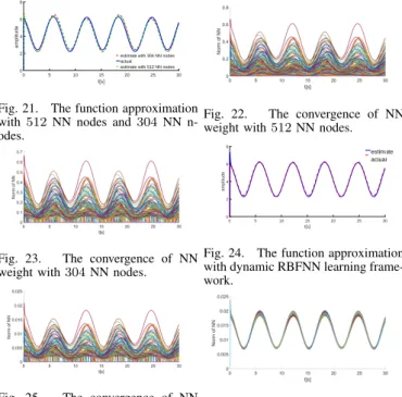
This group of experiments aims to test the function approxi-mation capabilities of RBFNN learning with dynamic updating algorithm. The RBFNN is employed to approximate the non-linear function f(q,q, α,˙ α˙) =Mq(q) ˙α+Cq(q,q˙)α+Gq(q),
whereαis defined in (24). The functional approximation per-formance of the our implemented neural network is depicted as shown in Figs. 21-26. The RBF network contains 512
nodes and parameters in updating law are set: Θ(·) = 0.03
σ= 0.035. The parameter of discarding nodes defined in (29)
is Υ = 0.05. As shown in Fig. 22, the weight of NN nodes
with their centers close to the input trajectory are activated well and the weight of NN nodes with their centers far away from the input trajectory are updating slightly and remains very small, that means, little learning experience can be obtained. In this case, we discard the NN nodes with their centers far away from the input trajectory according to the principle in (29), and the number of the discarded NN nodes is208. After discarding
0 5 10 15 20 25 30 t[s] 0 2 4 6 8 amplitude
estimate with 304 NN nodes actual estimate with 512 NN nodes
Fig. 21. The function approximation
with512 NN nodes and304NN
n-odes.
Fig. 22. The convergence of NN
weight with512NN nodes.
Fig. 23. The convergence of NN
weight with304NN nodes.
0 5 10 15 20 25 30 t[s] 0 2 4 6 8 amplitude estimate actual
Fig. 24. The function approximation
with dynamic RBFNN learning frame-work.
Fig. 25. The convergence of NN
weight with304NN nodes under
dy-namic RBFNN learning framework.
Fig. 26. The convergence of NN
weight of100new NN nodes.
these NN nodes, the function approximation performance (red dotted line) is shown in Fig. 21 and the weight convergence is shown in Fig. 23. Comparing the approximation performance before (green dotted line) and after (red dotted line) discarding nodes as shown in Fig. 21, we can see that the performance of neural network function approximation is affected little after discarding these nodes, but the computational burden of the system has been reduced in half. From the Fig. 21, it is seen that the function approximation performance is not very satis-factory. To make the neural network have better approximation ability,100new nodes are added into system with their centers next to the input trajectory, and the approximation results are depicted in Fig. 24. The value of weight is updating according to the law in (27), and the convergence of the weight of old NN nodes and new NN nodes are shown in Figs. 25 and 26, respectively. By comparing the Fig. 21 with Fig. 24, we can see that the approximation performance (blue solid line in Fig. 24) of implemented neural network with dynamic framework could follow the approximated non-linear function’s dynamics (red dotted line) better, which can verify the effectiveness of our proposed method.
V. CONCLUSION
In this paper, a neural-learning-based sensorless control scheme in the presence of input deadzone is presented for robotic arm to interact with the unknown environment. An inverse-dynamics-based force observer integrating the flatted network with RBF is developed to estimate the external force from the environment. A dynamic RBFNN learning framework is developed to approximate the uncertainties of the system. This novel NN adaptive controller is presented in Section III. The proposed control scheme is validated through experiments on the Baxter robot in Section IV.
VI. APPENDIX
Consider the following Lyapunov candidate
V = 1 2e T 2Mqe2+ 1 2tr( ˜W T τΘτWτ˜ ) + 1 2tr( ˜W T MΘMWM˜ ) +1 2tr( ˜W T CΘCW˜C) + 1 2tr( ˜W T GΘGW˜G) (32) The derivative of (32) is ˙ V =eT2Mqe˙2+ 1 2e T 2Mq˙ e2+tr( ˜WτTΘτWτ˙ˆ ) +tr( ˜WMTΘMW˙ˆM) +tr( ˜WCTΘCW˙ˆC) +tr( ˜WGTΘGWG˙ˆ ) (33)
Substituting (31) into (33), we have
˙ V =eT2(−M˜α˙−Cα˜ −G˜+ ∆ˆτ) −eT2K2e2−eT2∆τe+tr( ˜WτTΘτW˙ˆτ) +tr( ˜WMTΘMWM˙ˆ ) +tr( ˜WCTΘCWC˙ˆ ) +tr( ˜WGTΘGWG˙ˆ ) (34)
Substituting the NN updating law (27) into (34), yields
˙ V =−eT2(K2e2+ ∆τe−∆ˆτ)−eT2M˜α˙ −eT2Cα˜ −eT2G˜+tr( ˜WMTΘMW˙ˆM) +tr( ˜WCTΘCWC˙ˆ ) +tr( ˜WGTΘGWG˙ˆ ) =−eT2(K2e2+ ∆τe−∆ˆτ)−eT2M˜α˙ −eT2Cα˜ −e T 2G˜+tr[ ˜W T τ (S(Xτ)e2−στWτˆ )] +tr[ ˜WMT(S(XM) ˙αe2−σMWˆM)] +tr[ ˜WCT(S(XC)αe2−σCWCˆ )] +tr[ ˜WGT(S(XG)e2−σGWGˆ )] =−eT2K2e2−eT2∆τe−σMtr( ˜W T MWM˜ ) −σMtr( ˜WMTWM∗)−σCtr( ˜WCTWC˜ ) −σCtr( ˜WCTWC∗)−σGtr( ˜WGTW˜G) −σGtr( ˜WGTWG∗)−στtr( ˜WτTWτ˜ ) −στtr( ˜WτTWτ∗) (35)
Using the Youngs inequality [46], and the derivative ofV
is ˙ V ≤ −eT2K2e2+ 1 2e T 2e2− 1 2στtr( ˜W T τWτ˜ ) −1 2σMtr( ˜W T MW˜M)− 1 2σCtr( ˜W T CW˜C) −1 2σGtr( ˜W T GWG˜ ) + ∆ (36) where ∆ = 12∆τT e∆τe + 1 2σMtr(W ∗T M WM∗) + 1 2σCtr(W ∗T C WC∗) + 1 2σGtr(W ∗T G WG∗) + 1 2στtr(W ∗T τ Wτ∗).
Let us define $ comprised of e2,WM˜ ,WC,˜ WG˜ , and the
(36) can be rewritten asV˙ ≤ −κι($)+∆, whereκand∆are positive constant. There is an invariant setΩs for−κι($) + ∆>0, that is, the derivative ofV is negative outside the set. We can define the setΩbwithV($)decreasing inV <˙ 0, after
a period of time, the states$ will enter intoΩsand will not
escape afterwards. By uniformly ultimately bounded (UUB) stablity, the state variable$ will converge to a bounded set.
The invariant set can be defined as
Ωs= n (||W˜M||,||W˜C||,||W˜G||,||W˜τ||,||e2||), | eT 2(K2−12I)e2 ∆ + σD||W˜D||2 ∆ + σ∆||W˜C||2 ∆ +σG|| ˜ WG||2 ∆ + στ||Wτ˜ ||2 ∆ ≤1} (37)
As depicted in Fig. 5, the area of the set Ωs is in the first
quadrant passing through the points
σ(·)||W˜(·)||2= ∆, W˜ =ς
eT2(K2−
1
2I)e2= ∆, e2=ϑ
(38)
After new enhancement nodes are added into networks, we reconstruct a new Lyapunov candidate
V =1 2e T 2Mqe2+ 1 2tr( ˜W T τ nΘτ nWτ n˜ ) +1 2tr( ˜W T M NΘM NW˜M N) +1 2tr( ˜W T CNΘCNWCN˜ ) +1 2tr( ˜W T GNΘGNW˜GN) (39)
where W(·) denotes the NN weight after adding new nodes
into networks. The derivative of (39) is ˙ V =eT2Mqe˙2+ 1 2e T 2M˙qe2+tr( ˜Wτ nTΘτ nW˙ˆτ n) +tr( ˜WM NT ΘM NWM N˙ˆ ) +tr( ˜WCNT ΘCNWCN˙ˆ ) +tr( ˜WGNT ΘGNWGN˙ˆ ) (40)
Substituting (28) into (40) and noting that
˙ V =eT2(−M˜α˙ −Cα˜ −G˜+ ∆ˆτ)−eT2K2e2 −eT2∆τe+tr ˜ Wτ ˜ Wτ new T Θτ n " ˙ˆ Wτ ˙ˆ Wτ new #! +tr ˜ WM ˜ WM new T ΘM N " ˙ˆ WM ˙ˆ WM new #! +tr ˜ WC ˜ WCnew T ΘCN " ˙ˆ WC ˙ˆ WCnew #! +tr ˜ WG ˜ WGnew T ΘGN " ˙ˆ WG ˙ˆ WGnew #! (41) whereW(·new)denotes the weight vector of new added nodes.
The updating law is designed as
˙ˆ WM N = Θ−M N1 (S(XM N) ˙αe2−σM NWˆM N) ˙ˆ WCN = Θ−CN1(S(XCN)αe2−σCNWˆCN) ˙ˆ WGN = Θ−GN1(S(XGN)e2−σGNWGNˆ ) ˙ˆ Wτ n=−Θ−τ n1(S(Xτ n)e2+στ nWτ nˆ ) (42)
whereΘ(·)are positive definite matrices, and σ(·)are positive
Substituting (42) into (41), we have ˙ V =−eT2(K2e2+ ∆τe−∆ˆτ)−eT2M˜α˙ −eT2Cα˜ −eT2G˜+tr( ˜WM NT ΘM NW˙ˆM N) +tr( ˜WCNT ΘCNWCN˙ˆ ) +tr( ˜WGNT ΘGNWGN˙ˆ ) =−eT2K2e2−eT2∆τe−σM Ntr( ˜W T M NWM N˜ ) −σM Ntr( ˜WM NT WM N∗ )−σCNtr( ˜WCNT W˜CN) −σCNtr( ˜WCNT WCN∗ )−σGNtr( ˜WGNT W˜GN) −σGNtr( ˜WGNT WGN∗ )−στ ntr( ˜Wτ nTWτ n˜ ) −στ ntr( ˜Wτ nTWτ n∗ ) (43)
By using the Young’s inequality in (43), yields
˙ V ≤ −eT2K2e2+ 1 2e T 2e2− 1 2στ ntr( ˜W T τ nWτ n˜ ) −1 2σM Ntr( ˜W T M NW˜M N)− 1 2σCNtr( ˜W T CNW˜CN) −1 2σGNtr( ˜W T GNWGN˜ ) + ∆n (44) where ∆n = 12∆τeT∆τe + 1 2σM Ntr(W ∗T M NWM N∗ ) + 1 2σCNtr(W ∗T CNWCN∗ ) + 1 2σGNtr(W ∗T GNWGN∗ ) + 1 2στ ntr(W ∗T
τ nWτ n∗ ). We can find that the states after
adding new enhancement nodes also satisfy uniformly ultimately bounded(UUB) stablity. By using Theorem 1, we can prove that the states W˜τ n,W˜M N,W˜CN,W˜GN, e2 will
converge to an invariant set.
REFERENCES
[1] W. He, Z. Li, and C. P. Chen, “A survey of human-centered intelligent
robots: issues and challenges,”IEEE/CAA Journal of Automatica Sinica,
vol. 4, no. 4, pp. 602–609, 2017.
[2] Z. Li, S. S. Ge, and A. Ming, “Adaptive robust motion/force control
of holonomic-constrained nonholonomic mobile manipulators,” IEEE
Transactions on Systems, Man, and Cybernetics, Part B (Cybernetics), vol. 37, no. 3, pp. 607–616, 2007.
[3] J. J. Craig and M. H. Raibert, “A systematic method of hybrid
position/-force control of a manipulator,” inCOMPSAC 79. Proceedings.
Com-puter Software and The IEEE ComCom-puter Society’s Third International Applications Conference, 1979. IEEE, 1979, pp. 446–451.
[4] S. Part, “Impedance control: An approach to manipulation,”Journal of
dynamic systems, measurement, and control, vol. 107, no. 17, 1985. [5] J. E. Colgate and N. Hogan, “Robust control of dynamically interacting
systems,” International journal of Control, vol. 48, no. 1, pp. 65–88,
1988.
[6] M. T. Mason, “Compliance and force control for computer controlled
manipulators,”IEEE Transactions on Systems, Man, and Cybernetics,
vol. 11, no. 6, pp. 418–432, 1981.
[7] I. Ranatunga, F. L. Lewis, D. O. Popa, and S. M. Tousif, “Adaptive admittance control for humanvrobot interaction using model reference
design and adaptive inverse filtering,” IEEE Transactions on Control
Systems Technology, vol. 25, no. 1, pp. 278–285, Jan 2017.
[8] P. Marayong, G. D. Hager, and A. M. Okamura, “Control methods for guidance virtual fixtures in compliant human-machine interfaces,” in2008 IEEE/RSJ International Conference on Intelligent Robots and Systems, Sep. 2008, pp. 1166–1172.
[9] B. J. Waibel and H. Kazerooni, “Theory and experiments on the stability
of robot compliance control,” IEEE Transactions on Robotics and
Automation, vol. 7, no. 1, pp. 95–104, 1991.
[10] S. Eppinger and W. Seering, “Introduction to dynamic models for robot
force control,”IEEE Control Systems Magazine, vol. 7, no. 2, pp. 48–52,
1987.
[11] C. Lee, S. Chan, and D. Mital, “A joint torque disturbance observer
for robotic assembly,” inProceedings of 36th Midwest Symposium on
Circuits and Systems. IEEE, 1993, pp. 1439–1442.
[12] T. Murakami, R. Nakamura, F. Yu, and K. Ohnishi, “Force sensorless
impedance control by disturbance observer,” inConference Record of
the Power Conversion Conference-Yokohama 1993. IEEE, 1993, pp. 352–357.
[13] P. Hacksel and S. Salcudean, “Estimation of environment forces and
rigid-body velocities using observers,” inProceedings of the 1994 IEEE
International Conference on Robotics and Automation. IEEE, 1994, pp. 931–936.
[14] M. Capurso, M. M. G. Ardakani, R. Johansson, A. Robertsson, and P. Rocco, “Sensorless kinesthetic teaching of robotic manipulators
assisted by observer-based force control,” in2017 IEEE International
Conference on Robotics and Automation (ICRA). IEEE, 2017, pp. 945– 950.
[15] X. Liu, F. Zhao, S. S. Ge, Y. Wu, and X. Mei, “End-effector force estimation for flexible-joint robots with global friction approximation
using neural networks,”IEEE Transactions on Industrial Informatics,
vol. 15, no. 3, pp. 1730–1741, March 2019.
[16] V. Zahn, R. Maass, M. Dapper, and R. Eckmiller, “Learning friction estimation for sensorless force/position control in industrial
manipula-tors,” inProceedings 1999 IEEE International Conference on Robotics
and Automation (Cat. No. 99CH36288C), vol. 4. IEEE, 1999, pp. 2780–2785.
[17] A. C. Smith, F. Mobasser, and K. Hashtrudi-Zaad,
“Neural-network-based contact force observers for haptic applications,”IEEE
Transac-tions on Robotics, vol. 22, no. 6, pp. 1163–1175, 2006.
[18] Y.-H. Pao, G.-H. Park, and D. J. Sobajic, “Learning and generalization
characteristics of the random vector functional-link net,”
Neurocomput-ing, vol. 6, no. 2, pp. 163–180, 1994.
[19] C. L. P. Chen and J. Z. Wan, “A rapid learning and dynamic stepwise updating algorithm for flat neural networks and the application to
time-series prediction,”IEEE Transactions on Systems, Man, and Cybernetics,
Part B (Cybernetics), vol. 29, no. 1, pp. 62–72, Feb 1999.
[20] C.-E. Ren and C. P. Chen, “Sliding mode leader-following consensus
controllers for second-order non-linear multi-agent systems,”IET
Con-trol Theory & Applications, vol. 9, no. 10, pp. 1544–1552, 2015. [21] C. P. Chen, G.-X. Wen, Y.-J. Liu, and F.-Y. Wang, “Adaptive consensus
control for a class of nonlinear multiagent time-delay systems using
neural networks,”IEEE Transactions on Neural Networks and Learning
Systems, vol. 25, no. 6, pp. 1217–1226, 2014.
[22] Z. Li, S. Xiao, S. S. Ge, and H. Su, “Constrained multilegged robot system modeling and fuzzy control with uncertain kinematics and
dynamics incorporating foot force optimization,”IEEE Transactions on
Systems, Man, and Cybernetics: Systems, vol. 46, no. 1, pp. 1–15, 2015. [23] Z. Liu, G. Lai, Y. Zhang, and C. L. P. Chen, “Adaptive neural output feedback control of output-constrained nonlinear systems with unknown
output nonlinearity,”IEEE Transactions on Neural Networks and
Learn-ing Systems, vol. 26, no. 8, pp. 1789–1802, 2015.
[24] D.-P. Li, D.-J. Li, Y.-J. Liu, S. Tong, and C. P. Chen, “Approximation-based adaptive neural tracking control of nonlinear mimo unknown
time-varying delay systems with full state constraints,”IEEE transactions on
cybernetics, vol. 47, no. 10, pp. 3100–3109, 2017.
[25] A. M. Smith, C. Yang, H. Ma, P. Culverhouse, A. Cangelosi, and E. Bur-det, “Novel hybrid adaptive controller for manipulation in complex
perturbation environments,”PloS one, vol. 10, no. 6, 2015.
[26] C. Yang, X. Wang, L. Cheng, and H. Ma, “Neural-learning-based
telerobot control with guaranteed performance,”IEEE Transactions on
Cybernetics, vol. 47, no. 10, pp. 3148–3159, Oct 2017.
[27] C. Yang, Y. Jiang, Z. Li, W. He, and C. Su, “Neural control of bimanual
robots with guaranteed global stability and motion precision,” IEEE
Transactions on Industrial Informatics, vol. 13, no. 3, pp. 1162–1171, June 2017.
[28] C. Yang, X. Wang, Z. Li, Y. Li, and C. Su, “Teleoperation control
based on combination of wave variable and neural networks,” IEEE
Transactions on Systems, Man, and Cybernetics: Systems, vol. 47, no. 8, pp. 2125–2136, Aug 2017.
[29] Z. Li, Y. Xia, and F. Sun, “Adaptive fuzzy control for multilateral cooperative teleoperation of multiple robotic manipulators under random
network-induced delays,”IEEE Transactions on Fuzzy Systems, vol. 22,
no. 2, pp. 437–450, April 2014.
[30] C. L. P. Chen and Z. Liu, “Broad learning system: An effective and efficient incremental learning system without the need for deep
architecture,” IEEE Transactions on Neural Networks and Learning
Systems, vol. 29, no. 1, pp. 10–24, Jan 2018.
[31] C. L. P. Chen, Z. Liu, and S. Feng, “Universal approximation capability
of broad learning system and its structural variations,”IEEE
Transac-tions on Neural Networks and Learning Systems, vol. 30, no. 4, pp. 1191–1204, April 2019.
[32] Cong Wang and D. J. Hill, “Learning from neural control,” IEEE
Transactions on Neural Networks, vol. 17, no. 1, pp. 130–146, Jan 2006. [33] F. L. Lewis, Woo Kam Tim, Li-Zin Wang, and Z. X. Li, “Deadzone compensation in motion control systems using adaptive fuzzy logic
control,” IEEE Transactions on Control Systems Technology, vol. 7,
no. 6, pp. 731–742, Nov 1999.
[34] P. L. Andrighetto, A. C. Valdiero, and D. Bavaresco, “Dead zone
compensation in pneumatic servo systems,” inABCM symposium series
[35] R. R. Selmic and F. L. Lewis, “Deadzone compensation in motion
control systems using neural networks,”IEEE Transactions on Automatic
Control, vol. 45, no. 4, pp. 602–613, April 2000.
[36] W. He, A. O. David, Z. Yin, and C. Sun, “Neural network control of a
robotic manipulator with input deadzone and output constraint,”IEEE
Transactions on Systems, Man, and Cybernetics: Systems, vol. 46, no. 6, pp. 759–770, June 2016.
[37] S. I. Han and J. M. Lee, “Precise positioning of nonsmooth dynamic systems using fuzzy wavelet echo state networks and dynamic surface
sliding mode control,” IEEE Transactions on Industrial Electronics,
vol. 60, no. 11, pp. 5124–5136, Nov 2013.
[38] Y. Liu, L. Tang, S. Tong, and C. L. P. Chen, “Adaptive nn controller
design for a class of nonlinear mimo discrete-time systems,” IEEE
Transactions on Neural Networks and Learning Systems, vol. 26, no. 5, pp. 1007–1018, May 2015.
[39] G. Peng, C. Yang, W. He, and C. L. P. Chen, “Force sensorless admit-tance control with neural learning for robots with actuator saturation,”
IEEE Transactions on Industrial Electronics, pp. 1–1, 2019.
[40] B. Siciliano and O. Khatib,Springer handbook of robotics. Springer,
2016.
[41] S. G. Shuzhi, C. C. Hang, and L. Woon, “Adaptive neural network
control of robot manipulators in task space,” IEEE transactions on
industrial electronics, vol. 44, no. 6, pp. 746–752, 1997.
[42] T. H. Lee and C. J. Harris,Adaptive neural network control of robotic
manipulators. World Scientific, 1998, vol. 19.
[43] H. Huang, T. Zhang, C. Yang, and C. L. P. Chen, “Motor learning
and generalization using broad learning adaptive neural control,”IEEE
Transactions on Industrial Electronics, pp. 1–1, 2019.
[44] A. Smith, C. Yang, C. Li, H. Ma, and L. Zhao, “Development of
a dynamics model for the baxter robot,” in 2016 IEEE International
Conference on Mechatronics and Automation, Aug 2016, pp. 1244– 1249.
[45] Z. Ju, C. Yang, and H. Ma, “Kinematics modeling and experimental
verification of baxter robot,” inProceedings of the 33rd Chinese Control
Conference, July 2014, pp. 8518–8523.
[46] W. H. Young, “On classes of summable functions and their fourier
se-ries,”Proceedings of the Royal Society of London. Series A, Containing
Papers of a Mathematical and Physical Character, vol. 87, no. 594, pp. 225–229, 1912.
Guangzhu Pengreceived the B.Eng. degree in
au-tomation from Yangtze University, Jingzhou, China, in 2014, and the M.Eng. degree in pattern recogni-tion and intelligent systems from the College of Au-tomation Science and Engineering, South China U-niversity of Technology (SCUT), Guangzhou, China, in 2018. He is currently pursuing the Ph.D. degree in Computer Science with the Faculty of Science and Technology, University of Macau, Macau, China.
His current research interests include robotics, human-robot interaction, intelligent control, etc.
C. L. Philip Chen(S’88-M’88-SM’94-F’07) is the
Chair Professor and Dean of the School of Computer Science and Engineering, South China University of Technology, China; on leave from Faculty of Sci-ence and Technology, University of Macau, Macau, China. The University of Macau’s Engineering and Computer Science programs receiving Hong Kong Institute of Engineers’ (HKIE) accreditation and Washington/Seoul Accord is his utmost contribu-tion in engineering/computer science educacontribu-tion for Macau as the former Dean of the Faculty. His current research interests include systems, cybernetics, and compu-tational intelligence. Dr. Chen was the IEEE SMC Society President from 2012 to 2013 and is now a Vice President of Chinese Association of Automation (CAA). He is a Fellow of IEEE, AAAS, IAPR, CAA, and HKIE. He is the editor-in-chief of the IEEE Transactions on Cybernetics, and an associate editor of several IEEE Transactions. He was a Program Evaluator of the Accreditation Board of Engineering and Technology Education (ABET) of the U.S. for computer engineering, electrical engineering, and software engineering programs. He received 2016 Outstanding Electrical and Computer Engineers award from his alma mater, Purdue University after he graduated from the University of Michigan, Ann Arbor, Michigan, USA.
Wei He (S’09-M’12-SM’16) received his B.Eng.
and his M.Eng. degrees from College of Automation Science and Engineering, South China University of Technology (SCUT), China, in 2006 and 2008, respectively, and his PhD degree from Department of Electrical & Computer Engineering, the National University of Singapore (NUS), Singapore, in 2011. He is currently working as a full professor in School of Automation and Electrical Engineering, Univer-sity of Science and Technology Beijing, Beijing, China. He has co-authored 3 books published in Springer and published over 100 international journal and conference papers. He was awarded a Newton Advanced Fellowship from the Royal Society, UK in 2017. He was a recipient of the IEEE SMC Society Andrew P. Sage Best Transactions Paper Award in 2017. He is serving the Chair of IEEE SMC Society Beijing Capital Region Chapter. He is serving as an Associate
Editor ofIEEE Transactions on Neural Networks and Learning Systems,IEEE
Transactions on Control Systems Technology,IEEE Transactions on Systems, Man, and Cybernetics: Systems,Assembly Automation,IEEE/CAA Journal of Automatica Sinica,Neurocomputing, and an Editor ofJournal of Intelligent & Robotic Systems. His current research interests include robotics, distributed parameter systems and intelligent control systems.
Chenguang Yang (M’10-SM’16) received the
B.Eng. degree in measurement and control from Northwestern Polytechnical University, Xian, China, in 2005, the Ph.D. degree in control engineering from the National University of Singapore, Singa-pore, in 2010 and postdoctoral training in human robotics from the Imperial College London, London, U.K. He has been awarded EU Marie Curie Inter-national Incoming Fellowship, UK EPSRC UKRI Innovation Fellowship, and the Best Paper Award of the IEEE Transactions on Robotics as well as over ten conference Best Paper Awards. His research interest lies in human robot interaction and intelligent system design.
![Fig. 1. The structure and updating algorithm for Functional-link neural network (modified from [19]).](https://thumb-us.123doks.com/thumbv2/123dok_us/10953577.2983837/3.892.81.430.89.268/fig-structure-updating-algorithm-functional-neural-network-modified.webp)
![Fig. 2. The deadzone nonlinearity (modified from [36]).](https://thumb-us.123doks.com/thumbv2/123dok_us/10953577.2983837/4.892.472.812.105.273/fig-the-deadzone-nonlinearity-modified-from.webp)