Structural Properties of Transmuted Weibull Distribution

Volume 14 | Issue 2 Article 13

11-1-2015

Structural Properties of Transmuted Weibull

Distribution

Kaisar Ahmad

University of Kashmir, Srinagar, India, [email protected]

S. P. Ahmad

University of Kashmir, Srinagar, India, [email protected]

A. Ahmed

Aligarh Muslim University, Aligarh, India

Follow this and additional works at:http://digitalcommons.wayne.edu/jmasm

Part of theApplied Statistics Commons,Social and Behavioral Sciences Commons, and the Statistical Theory Commons

Recommended Citation

Ahmad, Kaisar; Ahmad, S. P.; and Ahmed, A. (2015) "Structural Properties of Transmuted Weibull Distribution,"Journal of Modern Applied Statistical Methods: Vol. 14 : Iss. 2 , Article 13.

DOI: 10.22237/jmasm/1446351120

K. Ahmad and S. P. Ahmad are in the Department of Statistics. Email at

[email protected] and [email protected], respectively. A. Ahmed is in the Department of Statistics and O.R.

Structural Properties of Transmuted Weibull

Distribution

Kaisar Ahmad University of Kashmir Srinagar, India S. P. Ahmad University of Kashmir Srinagar, India A. Ahmed

Aligarh Muslim University Aligarh, India

The transmuted Weibull distribution, and a related special case, is introduced. Estimates of parameters are obtained by using a new method of moments.

Keywords: Transmuted Weibull distribution, moment generating function, sample

coefficient of variation, Standard deviation, Skewness and kurtosis

Introduction

The Weibull distribution was introduced by the Swedish Physicist Waloddi Weibull in 1939. He applied this distribution to analyze the breaking strength of materials. This distribution has been extensively used in lifetime and reliability problem. The Weibull family is a generalization of the exponential family and can model data exhibiting monotone hazard rate behavior, i.e., it can accommodate three types of failure rates, namely increasing, decreasing and constant. Its application in connection with lifetimes of many types of manufactured items has been widely advocated (e.g., Weibull, 1951; Berrettoni, 1964), and it has been used as a model with diverse types of items such as vacuum tubes (Kao, 1959), ball bearings (Lieblein & Zelen, 1956), and electrical insulation. It is also widely used in biomedical applications.

A simple explanation of the Weibull distribution and its applications can be found in Franck (1988). A comprehensive review of this model is available in Johnson, Kotz, and Balakrishnan (1995). A generalization of the Weibull distribution with application to the analysis of survival data is given by Mudholkar, Srivastava, and Kollia (1996). Inferences from grouped data in the three-parameter Weibull models is introduced by Hirose and Lai (1997). Lawless

(2002) provided statistical models and methods for lifetime data. Al-Athari (2011) and Hossain and Zimmer (2003) did some comparative studies on the estimation of Weibull parameters using complete and censored samples. Nadarajah and Kotz (2005) presented a procedure on some recent modifications of Weibull distribution.

For deriving new moment estimators of three parameters transmuted Weibull distribution, a similar approach to that of Huang and Hwang (2006) was used. Nadarajah and Kotz (2005) discussed products and ratios of Weibull random variables. Gokarna and Tsokos (2009) proposed a method on the transmuted extreme value distribution with application. Ahmad and Ahmad (2013) presented a procedure of Bayesian analysis of Weibull distribution.

A random variable x is said to have a Weibull distribution with parameters

α > 0 and β > 0 if its pdf is given by

 

1 exp x 0, 0, 0 g x x x    _{ }       _ _     

The cdf of Weibull distribution is given by

 

 

0 x G x 



g x dx

 

1 0 exp x x G x x dx          _ _  



⇒

G x

 

1 exp x       _ _   (1)

Transmuted Weibull distribution

In order to obtain the pdf of transmuted Weibull distribution, use the following cdf which is given by

  

  

 

2

1

where G(x) is the cdf of base distribution. If λ = 0, we have the distribution of base random variable.

Now using equation (1) in equation (2),

  



2 1 1 exp x 1 exp x F x                              

⇒

  



2 1 F x  



k



k where 1 exp x k       _ _  

⇒

F x

 

k



1 

 

k



⇒

F x

 

k



1





1k





⇒

F x

 

1 exp x 1 exp x  







        _  _ _  _ _         (3)

This is the required cdf of Transmuted Weibull distribution.

In order to find the pdf of Transmuted Weibull distribution, first differentiate equation (3) w.r.t. x which is given by

 

d



 



f x F x dx 

⇒

f x

 

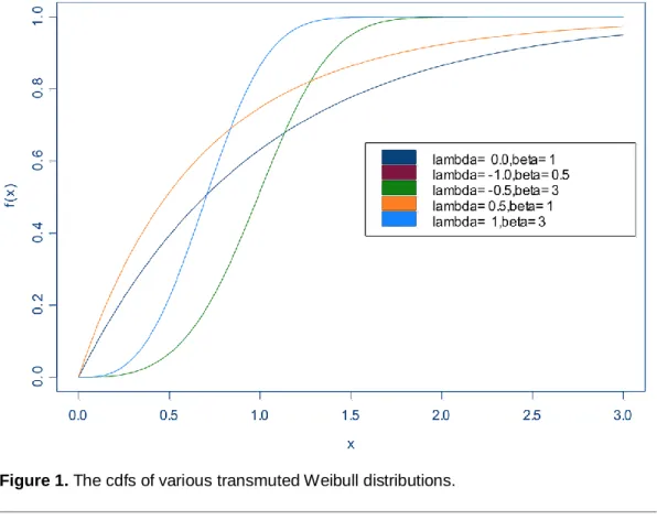
d 1 exp x 1 exp x dx                            

Figure 1. The cdfs of various transmuted Weibull distributions.

After differentiating the above equation w.r.t. x,

 

1 exp x 1 2 exp x f x x   



_

_







      _ _   _ _       (4)

which is the required pdf of Transmuted Weibull distribution with parameters α, β and λ.

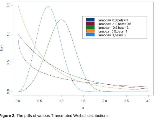
Figure 2. The pdfs of various Transmuted Weibull distributions.

Special cases

1) If λ = 0, then Transmuted Weibull distribution reduced to two parameter Weibull distribution with parameters α and β.





1 ; , exp x 0 , 0 f x x x              _ _    

2) If λ = 0 and β = 1, then Transmuted Weibull distribution reduced to exponential distribution with parameter 1



     , i.e.

 

1 exp x 0, 0 f x x







   _ _    

3) If λ = 0 and α = β = 1, then Transmuted Weibull distribution reduced to standard exponential distribution, i.e.

 

exp

 

0

f x  x x Moments of Transmuted Weibull distribution

Moments are the expected values of certain functions of a random variable. They serve to numerically describe the variable with respect to given characteristics for location, variation, skewness and kurtosis, to name a few. The expected value of

xr _{is termed as r}th _{moment about origin of the random variable x which is given by}

 

r

r E x

 

Thus the rth _{moment of Transmuted Weibull distribution is given by}





0 ; , , r r x f x dx  

_

   1 0 exp 1 2 exp r r x x x x dx   















        _ _   _ _      



After solving the above equation,





1 1 2 r r r r  





 



     _  _     (5)

Mean of the Transmuted Weibull distribution

Setting r = 1 in equation (5) leads to the mean of the Transmuted Weibull distribution, which is given by





1 1 1 1 1 1 2  

 

 



     _  _     (6)

Second moment of the Transmuted Weibull distribution Setting r = 2 in equation (5),





2 2 2 2 1 1 2  





 



     _  _     (7)

Variance of Transmuted Weibull distribution

The variance of Transmuted Weibull distribution is given by









2 2 1 2 2 2 2 1 1 1 2 1 1 2                     __  _     _  _   _       (8)

Third and fourth moments of Transmuted Weibull distribution Setting r = 3 in equation (5),





3 3 3 3 1 1 2  





 



     _  _     and

















3 3 2 1 1 3 2 2 3 1 1 2 2 3 1 1 2 1 1 1 2 1 2 1 1 2     

 







 



 



 



                     _{   }    _ _  _   _ _ _  _{ }               _{ }  _{      }     _{   }   (9) If r = 4 in equation (5),





4 4 4 4 1 1 2  





 



     _  _     thus

























4 3 4 1 1 2 1 2 4 3 3 4 1 1 2 3 4 1 1 2 1 6 1 1 2 1 1 1 2 2 1 1 2 1 3 1 1 2       

 



 







 



 



 



 



                       _{   }  _{      }  _{   }  _{ }    _{ }  _   _  _   _       _  _   _{ }    _ _  _{ }     _{ }    _{ }  _{   }       _{   }        (10)

MGF of Transmuted Weibull distribution

The mgf of Transmuted Weibull distribution is given by

 

 

0 tx x M t e f x dx  



 

   

2 3

 

 

0 1 2! 3! ! n x tx tx tx M t tx f x dx n _ _  _       _    



 

 

0 0 ! r r x r t x M t f x dx r    





 

 

0 !₀ r r x r t M t x f x dx r    

 

 

0 ! r x r r t M t r



   



 





0 1 1 2 ! r r r x r t r M t r  



 



 _     _  _    



(11)

This is the required mgf of Transmuted Weibull distribution. Standard deviation of Transmuted Weibull distribution

The positive square root of the variance is called standard deviation. Symbolically,

σ = 2

. From equation (8), the variance of Transmuted Weibull distribution is given as









2 2 1 2 2 2 2 1 1 1 2 1 1 2                     __  _     _  _   _      

⇒

1



2





1



2 2 2 1 1 1 2 1 1 2                     __  _     _  _   _      

⇒

1 2 2 1 

  

 



where





1 1 2 k k k 



 



    _  _     (12)

Coefficient of variation of Transmuted Weibull distribution

This is the ratio of standard deviation and mean. Usually, it is denoted by C.V. and is given by

. .

C V





⇒













1 2 1 1 1 2 2 2 1 1 1 2 1 1 2 . . 1 1 1 2 C V     



 

 







 



   _ _  _{   }  _  _{ }                 _  _    

⇒

2 12 1 . . C V      (13) where



_k k 1 1



 

21





    _  _    

Skewness and kurtosis of Transmuted Weibull distribution

The most popular way to measure the skewness and kurtosis of a distribution function rests upon ratios of moments. Lack of symmetry of tails (about mean) of frequency distribution curve is known as skewness. The formula for measure of skewness given by Karl Pearson in terms of moments of frequency distribution is given by 2 3 1 3 2    

After using equation (8) and equation (9) in the above equation, we have

























3 2 1 1 2 1 2 2 2 1 3 2 2 3 1 1 2 2 3 1 1 2 1 1 1 2 1 2 1 1 2 2 1      

 



 



 



 





 

 

      _ _  _{ }           _{   }  _ _  _   _ _ _  _{ }          _{ }    _{ }  _{      }     _{   }    _ _  _{   }  _  _{ } 

⇒













2 2 3 1 2 1 1 ₂ 3 2 1 3



 









    where



1



1 1 2 k k _



 



    _  _     Therefore 1 1   

⇒













3 2 2 3 1 2 1 1 2 2 1 3



 









   

If γ1 < 0, then the frequency curve is negatively skewed. If γ1 > 0, then the frequency curve is positively skewed.

Kurtosis

The formula for measure of kurtosis is given by

4 2 2 2









After using equation (8) and equation (10) in the above equation,

































4 3 1 1 2 1 2 1 3 3 2 2 2 2 4 1 1 2 1 3 1 1 2 4 1 1 2 1 2 6 1 1 2 1 1 2 1 3 1 1 2 2 1 1 1 2 1 1 2        

 



 

 





 

 





 





 

 





                          _  _   _ _  _              _  _   _  _   _         _   _  _   _                               

⇒













3 4 1 3 1 2 1 2 2 2 1 4 6 3               where



1



1 1 2 k k _



 



    _  _     and 2 2 3









⇒













3 4 1 3 1 2 1 2 2 2 1 4 6 3 3               

If γ2 > 0, then the frequency curve is leptokurtic. If γ2 < 0, then the frequency curve is platykurtic. If γ2 = 0, then the frequency curve is mesokurtic, or we can say that there is no kurtosis.

Harmonic mean of Transmuted Weibull distribution





0 1 ; , , f x dx H     



1 0 1 1 exp x 1 2 exp x x dx H x   



_

_







       _ _   _ _      







1 1 0 0 1 1 1 2 1 x exp x dx 2 x exp x dx H x x                       _ _  _ _    





After substitution,





1 1 0 0 1 1 1 1 2 exp z dz 2 exp z dz H _z _z          _{   }  _ _  _ _    





After solving the above equation





1 1 1 1 1 1 2 H  



 



     _{ }    

⇒





1 1 1 1 1 1 2 H  



 



     _{ }     (14)

New moment estimator of the Transmuted Weibull distribution

For deriving new moment estimators of three parameters transmuted Weibull distribution, we need the following theorem obtained by using the similar approach of Huang and Hwang (2006).

Theorem 1. Let n ≥ 3 and let X1, X2, X3, …, Xn be n positive identical

independently random variables having probability density function f (x). Then the independence of the sample mean

X

_n and the sample coefficient of variance

n n n S V X

 is equivalent to that f (x) is a Transmuted Weibull density where Sn is the

sample standard deviation.

The next theorem requires the derivation of the expectation and the variance of 2 2 n n n S V X     

  , where

X

n and Sn are respectively the sample mean and the

sample standard deviation.

Theorem 2. Let X1, X2, X3, …, Xn be n positive identical independently

distributed random samples drawn from a population having Transmuted Weibull density





1 ; , , exp x 1 2 exp x f x x   



  











      _ _   _ _       then

 

2



2





1



2 2 2 2 1 1 1 2 1 1 2 n E S                   __  _     _  _   _      

Proof: Because the rth _{moment of a random variable x about origin is given by}





0 ; , , r r x f x dx  

_

   1 0 exp 1 2 exp r r x x x x dx   















        _ _   _ _      



After solving the above equation,





1 1 2 r r r r  





 



     _  _    

 

1 1



1



1 1 2 n E X





 





    _  _    

Also if r = 2 in the above equation,

 













2 2 1 2 2 2 2 1 1 2 1 1 1 1 2 n n E X n             _ _  _{ }           _{ }         _{ }         (15) and

 









2 2 1 2 2 2 1 1 2 1 1 1 2 n V X n             _ _  _{ }              _{   }     _{ }     . Thus

 

2

 

n n E S nV X

 









2 2 1 2 2 2 2 1 1 2 1 1 1 2 n E S   

 





 



                   _{ }   _{   }     _{ }    (16)

where

X

_n and

S

_n2 are respectively the sample mean and the sample variance.

Theorem 3. Let X1, X2, X3, …, Xn be n positive identical independently

distributed random samples drawn from a population having Transmuted Weibull density





1 ; , , exp x 1 2 exp x f x x   



  











      _ _   _ _       then





















2 1 2 1 2 2 2 2 2 2 2 1 1 2 1 1 1 2 2 1 1 2 1 1 1 1 2 n n n S E X n    

 



 



 



 



    _ _  _{ }              _{   }        _{   }   _{  }     _{   }          _{ }         _{ }       

where

X

_n and

S

_n2 are respectively the sample mean and the sample variance.

Proof: By using the theorem (1), we have

 

2 2

 

2 2 2 2 2 n n n n n n n S S E S E X E E X X X      _{ } _{ }    

⇒

 

 

2 2 2 2 n n n n E S S E X E X        (17)





















2 1 2 1 2 2 2 2 2 2 2 1 1 2 1 1 1 2 2 1 1 2 1 1 1 1 2 n n n S E X n    

 



 



 



 



                        _{   }        _{   }   _{  }     _{   }          _{ }         _{ }       









2 1 2 2 ₂ 2 2 1 1 2 1 1 1 1 2 n n S E X                         _{   }     _{ }     _{   }        

as n  and that this limit is the square of the population coefficient of variation. Thus, 2 2 n n S

X is an asymptotically unbiased estimator of the square of the

population coefficient of variation.

References

Ahmad, S. P. & Ahmad, K. (2013). Bayesian analysis of Weibull

distribution using R software. Australian Journal of Basic and Applied Sciences, 7(9), 156-164. http://ajbasweb.com/old/ajbas/2013/July/156-164.pdf

Al-Athari, F. M. (2011). Parameter estimation for the double-Pareto distribution. Journal of Mathematics and Statistics, 7(4), 289–294.

doi:10.3844/jmssp.2011.289.294

Berrettoni, J. N. (1964). Practical applications of the Weibull distribution,

Industrial Quality Control, 21(2), 71-79.

Franck, J. R. (1988). A simple explanation of the Weibull distribution and its applications. Reliability Review, 8(3), 93-116.

Gokarna R. A. & Tsokos, C. P. (2009). On the transmuted extreme value distribution with application. Nonlinear Analysis: Theory, Methods and Applications, 71(12), e1401–e1407. doi:10.1016/j.na.2009.01.168

Hirose, H. & Lai, T. L. (1997). Inference from grouped data in three-parameter Weibull models with applications to breakdown-voltage experiments,

Technometrics, 39(2), 199-210. doi:10.1080/00401706.1997.10485085

Hossain, A. & Zimmer, W. (2003). Comparison of estimation methods for Weibull parameters: complete and censored samples. Journal of Statistical Computation and Simulation, 73(2), 145–153.

doi:10.1080/0094965021000033486

Huang, P. H. & Hwang, T. Y. (2006). On new moment estimation of

parameters of the generalized gamma distribution using it’s characterization. [sic]

Taiwanese Journal of Mathematics, 10(4), 1083 -1093.

Johnson, N. L., Kotz, S., & Balakrishnan, N. (1995). Continuous univariate distributions (Vol. 2). New York: John Wiley & Sons.

Kao, J. H. K. (1959). A graphical estimation of mixed Weibull parameters in life testing of electron tubes. Technometrics, 1(4), 389-407.

doi:10.1080/00401706.1959.10489870

Lawless, J. F. (2002). Statistical models and methods for lifetime data (2nd Ed.). New York: John Wiley & Sons.

Lieblein, J. & Zelen, M. (1956). Statistical investigation of the fatigue life of deep groove ball bearing. Journal of Research of the National Bureau of

Standards, 57(5),273-316. doi:10.6028/jres.057.033

Mudholkar, G. S., Srivastava, D. K. & Kollia, G. D. (1996). A

generalization of the Weibull distribution with application to the analysis of survival data. Journal of the American Statistical Association, 91(436), 1575-1583. doi:10.1080/01621459.1996.10476725

Nadarajah, S. & Kotz, S. (2005). On some recent modifications of Weibull distribution, IEEE Transactions on Reliability, 54(4), 561-562.

doi:10.1109/TR.2005.858811

Weibull, W. (1939). A statistical theory of strength of materials. Ingeniörs Vetenskapsakademien Handlingar, 151, 1-45.

Weibull, W. (1951). A statistical distribution function of wide applicability.