David C. Wyld et al. (Eds): CCSEA, BIoT, DKMP, CLOUD, NLCAI, SIPRO - 2020
pp. 175-194, 2020. CS & IT - CSCP 2020 DOI: 10.5121/csit.2020.101014
D
ERIVATION OF
L
OOP
G
AIN AND
S
TABILITY
T
EST FOR
L
OW
-P
ASS
T
OW
-T
HOMAS
B
IQUAD
F
ILTER
MinhTri Tran, Anna Kuwana and Haruo Kobayashi
Division of Electronics and Informatics,
Gunma University, Kiryu 376-8515, Japan
A
BSTRACTProposed derivation and measurement of self-loop function for a low-pass Tow Thomas biquadratic filter are introduced. The self-loop function of this filter is derived and analyzed based on the widened superposition principle. The alternating current conservation technique is proposed to measure the self-loop function. Research results show that the selected passive components (resistors, capacitors) of the frequency compensation of Miller’s capacitors in the operational amplifier and the Tow Thomas filter can cause a damped oscillation noise when the stable conditions for the transfer functions of these networks are not satisfied.
K
EYWORDSSuperposition, Self-loop Function, Stability Test, Tow-Thomas Biquadratic Filter, Voltage Injection.
1.
I
NTRODUCTIONAn important function of microelectronics vastly used in electronic systems is “filtering”[1]. One of the most famous active filter circuits is the Tow–Thomas bi-quadratic circuit. Although the circuit was introduced many years ago, it is still receiving interest of researchers in modifying it to fit the new CMOS technology [2]. Moreover, feedback control theories are widely applied in the processing of analogue signals [3]. In conventional analysis of a feedback system, the term of “Aβ(s)” is called loop gain when the denominator of the transfer function is simplified as 1+Aβ(s). The stability of a feedback network is determined by the magnitude and phase plots of the loop gain. However, the passive filter is not a closed loop system. Furthermore, the denominator of the transfer function of the analog filter, regardless of active or passive is also simplified as 1+L(s), where L(s) is called “self-loop function”. Therefore, the term of “self-loop function” is proposed to define L(s) for both cases with and without feedback filters. This paper provides an introduction to the derivation of the transfer function, the measurement of self-loop function and stability test for a low-pass Tow-Thomas biquadratic filter based on the alternating current-voltage injection technique and the widened superposition principle.
The main contribution of this paper comes from the stability test for a low-pass Two Thomas biquadratic filter based on the widened superposition and the voltage injection technique. Section 2 of the paper mathematically analyzes an illustrative second-order denominator complex function considered in details. Section 3 presents the stability test for a mathematical model of two-stage operational amplifier which is used in the Tow Thomas circuit. SPICE simulation results and the stability test for the Tow Thomas filter are described in Section 4. A brief
discussion of the research results is given in Section 5. The main points of this work are summarized in Section 6. We have collected a few important notions and results from analysis in an Appendix for easy references like A.1, A.2, etc.
2.
A
NALYSIS OFS
ECONDO
RDERD
ENOMINATORC
OMPLEXF
UNCTIONS2.1.
Widened Superposition Principle
In this section, we propose a new concept of the superposition principle which is useful when we derive the transfer function of a network. The conventional superposition theorem is used to find the solution to linear networks consisting of two or more sources (independent sources, linear dependent sources) that are not in series or parallel. To consider the effects of each source independently requires that sources be removed and replaced without affecting the final result. To remove a voltage source when applying this theorem, the difference in potential between the terminals of the voltage source must be set to zero (short circuit); removing a current source requires that its terminals be opened (open circuit). This procedure is followed for each source in turn, and then the resultant responses are added to determine the true operation of the circuit. There are some limitations of conventional superposition theorem. Superposition cannot be applied to power effects because the power is related to the square of the voltage across a resistor or the current through a resistor. Superposition theorem cannot be applied for non linear circuit (diodes or transistors). In order to calculate load current or the load voltage for the several choices of load resistance of the resistive network, one needs to solve for every source voltage and current, perhaps several times. With the simple circuit, this is fairly easy but in a large circuit this method becomes a painful experience.
In the paper, the nodal analysis on circuits is used to obtain multiple Kirchhoff current law equations. The term of "widened superposition" is proposed to define a general superposition principle which is the standard nodal analysis equation, and simplified for the case when impedance from node A to ground is infinity and current injection into node A is 0. In a circuit having more than one independent source, we can consider the effects of all the sources at a time. The widened superposition principle is used to derive the transfer function of a network [4,5]. Energy at one place is proportional with their input sources and the resistance distances of transmission spaces. Let EA(t) be energy at one place of multi-sources Ei(t) which are transmitted
on the different resistance distances di (R, ZL, and ZC in electronic circuits) of the transmission
spaces as shown in Figure 1. Widened superposition principle can be defined as
n n i A i=1 i i=1 i
E (t)
1
E (t)
=
d
d
(1)The import of these concepts into circuit theory is relatively new with much recent progress regarding filter theory, analysis and implementation.
1 d 2 d 3 d 4 d 5 d n d … 1 E (t) 2 E (t) 3 E (t) 4 E (t) 5 E (t) n E (t) A E (t)
2.2.
Analysis of Complex Functions
In this section, we describe a transfer function as the form of a complex function which the variable is an angular frequency. In frequency domain, the transfer function and the self-loop function of a filter are complex functions. Complex functions are typically represented in two forms: polar or rectangular. The polar form and the rectangular representation of a complex function H(jω) is written as Im arctan 2 2 Re Re Im Re Im H j j H j H j H j j H j H j H j e (2)
where Re{H(jω)} is the real part of H(jω) and Im{H(jω)} is the imaginary part of H(jω), and j is the imaginary operator j2 = -1. The real quantity 2 2
Re H j Im H j is known as the
amplitude or magnitude, the real quantity arctan Im Re
H j
H j is called the angle H j , which is
the angle between the real axis and
H j
. The angle may be expressed in either radians or degrees and real quantity ImReH jH j is called the argument Arg H j which is the ratio betweenthe real part and the imaginary part of H(jω). The operations of addition, subtraction, multiplication, and division are applied to complex functions in the same manner as that they are to complex numbers. Complex functions are typically expressed in three forms: magnitude-angular plots (Bode plots), polar charts (Nyquist charts), and magnitude-argument diagrams (Nichols diagrams). In the paper, the stability test is performed on the magnitude-angular charts.
2.3.
Second Order Denominator Complex Functions
In this section, we shall analyze the frequency response of a typical second order denominator complex function on the magnitude-angular charts. A general transfer function of the second-order denominator complex function is defined as in Equation (3). Assume that all constant variables are not equal to zero. If the constant is smaller than zero, the constant is expressed as a complex number (a 0 a a j2 a e j ). In the paper, the angular of the constant is not
written in details. 2
1
(
)
H s
j
as
bs c
(3)From Equation (24) in Appendix A.1, the simplified complex function is
2 2 2 2 4 ( ) 2 2 1 2 a b H j a a c b j b b a a (4)
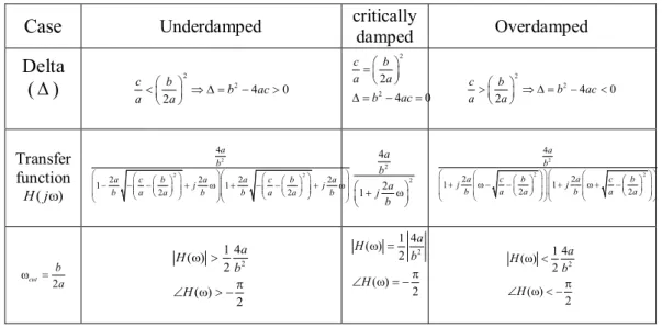
In order to plot the magnitude-angular charts, the values of magnitude-angular of the complex function, which are calculated in Appendix A.1, are summarized on Table 1.
In overdamped case, the magnitude of the complex function is so high from the first cut-off angular frequency 2 1 2 1 2 2 cut b a c b
a b a a
to
the second cut-off angular frequency2 2 2 1 2 2 cut b a c b
a b a a
.
Therefore, this gain will amplify the high order harmonics fromωcut1 to ωcut2 of an input signal which includes many harmonics.
Table 1. Summary of magnitude-angular values of second order denominator complex function.
Case
Underdamped critically damped OverdampedDelta
( )
2 2 4 0 2 c b b ac a a 2 2 2 4 0 c b a a b ac 2 2 4 0 2 c b b ac a a Transfer function ( ) H j 2 2 2 4 2 2 2 2 1 1 2 2 a b a c b j a a c b j a b a a b b a a b 2 2 4 2 1 a b a j b 2 2 2 4 2 2 1 1 2 2 a b a c b a c b j j b a a b a a 2 cut b a 2 1 4 ( ) 2 ( ) 2 a H b H 2 1 4 ( ) 2 ( ) 2 a H b H 2 1 4 ( ) 2 ( ) 2 a H b H2.4.
Damped Oscillation Noise
In this section, we describe the response of a typical second-order denominator complex function to a step input or a square wave.
Based on the Fourier series expansion of the square wave,
the waveforms of the pulse wave are expressed in many functions of time with many
different frequencies as shown in Figure 2.
f1 f3 f5 f t A 0 0.5T T (b) 0 A (a)
Fig. 2. Square wave: (a) waveform, spectrum, and (b) partial sums of Fourier series. The waveform function of a square wave is
1 1 sin 2 2 1 4 ( ) 2 1 k k f t S t k (5)
In under-damped case, the high-order harmonics of the step signal are significantly reduced from the first cut-off angular frequency. Therefore, the rising time and falling time is rather low. In this case, the system is absolutely stable.
In case of critically damped, the rising time and falling time are longer than the underdamped case. Now, the system is marginally stable. The energy propagation is also maximal because this condition is equal to the balanced charge-discharge time condition [6].
In over-damped case of the complex function, the gain at the cut-off angular frequency will amplify the high-order harmonics of the step signal that causes the peaking or ringing. Ringing is an unwanted oscillation of a voltage or current. The term of “damped oscillation noise” is proposed to define this unwanted oscillation which fades away with time, particularly in the step response (the response to a sudden change in input). Damped oscillation noise is undesirable because it causes extra current to flow, thereby wasting energy and causing extra heating of the components. It can cause unwanted electromagnetic radiation to be emitted. Therefore, the system is unstable.
2.5.
Graph Signal Model for General Denominator Complex Functions
In this section, we describe the graph signal model of a typical complex function which is the same as graph signal model of a feedback system. A negative-feedback amplifier is an electronic amplifier that subtracts a fraction of its output from its input, so that negative feedback opposes the original signal. The applied negative feedback can improve its performance (gain stability, linearity, frequency response, step response) and reduces sensitivity to parameter variations due to manufacturing or environment. Because of these advantages, many amplifiers and control systems use negative feedback. However, the denominator complex functions are also expressed in graph signal model which is the same as the negative feedback system. A general denominator complex function is rewritten as
( ) ( ) ( ) ( ) 1 ( ) out in V s A s H s V s L s (6) This form is called the standard form of the denominator complex function. The output signal is calculated as ( ) ( ) ( ) ( ) out in out L s V s A s V s V s A s (7)
Figure 3 presents the graph signal model of a general denominator complex function. The feedback system is unstable if the closed-loop “gain” goes to infinity, and the circuit can amplify its own oscillation. The condition for oscillation is
2 1
( )
1 1
j k;
L s
e
k Z
(8)Through the self-loop function, a second-order denominator complex function can be found that is stable or not. The concepts of phase margin and gain margin are used to asset the characteristics of the loop function at unity gain.
Figure 3. Graph signal model of general denominator complex function.
The conventional test of the loop gain (L(s) =
L s e
( )
j L s( )), which is called “Barkhausen’scriteria”, is unity gain and -180o of phase in magnitude-phase plots (Bode plots) [7].
2.6.
Self-loop Function of Second Order Denominator Complex Functions
In this section, we investigate the characteristics of the self-loop function L(s) on the magnitude-angular charts. The general transfer function and self-loop function are rewritten as
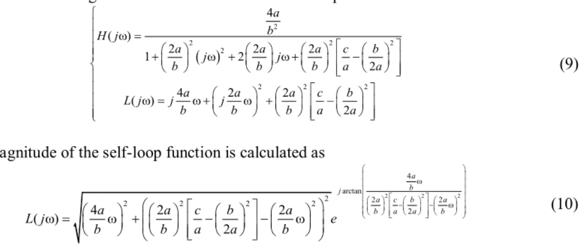
2 2 2 2 2 2 2 2 4 ( ) 2 2 2 1 2 2 4 2 2 ( ) 2 a b H j a a a c b j j b b b a a a a a c b L j j j b b b a a (9)
The magnitude of the self-loop function is calculated as
2 2 2 4 arctan 2 2 2 2 2 2 2 2 4 2 2 ( ) 2 a b j a c b a b a a b a a c b a L j e b b a a b (10)
The values of magnitude and angular of the self-loop function, which are calculated in Appendix A.2, are summarized in Table 2. In this work, the self-loop function is only sketched on the magnitude-angular charts.
Table 2. Summary of magnitude-angular values of self-loop function
Self-loop function ( ) L j 2 2 2 2 2 2 2 2 4 4 2 2 ( ) ; ( ) arctan 2 2 2 2 a a a c b a b L j L j b b a a b a c b a b a a b Delta( ) 2 2 4 0 2 c b b ac a a 2 2 4 0 2 c b b ac a a 2 2 4 0 2 c b b ac a a 5 2 2 b a L( ) 1 L( ) 76.3o L( ) 1 L( ) 76.3o L( ) 1 ( ) 76.3 o L 2 b a L( ) 5 ( ) 63.4o L ( ) 5 L ( ) 63.4 o L ( ) 5 L ( ) 63.4 o L
b a ( ) 4 2 L ( ) 45o L L( ) 4 2 L( ) 45o L( ) 4 2 L( ) 45o
2.7.
Comparison Measurement
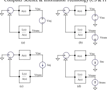
In this section, we describe a mathematical way to derive the self-loop function through the open loop function A(s) and the closed loop transfer function. In the conventional ways, such as voltage injection, replica measurement is used to measure the loop gain of a feedback loop [8,9]. However, from mathematical analysis the self-loop function can be derived by the comparison measurement method [10]. In other words, loop gain can be withdrawn by the open loop function A(s) and the closed loop transfer function without breaking the feedback loop as shown in Fig. 4. From Equation (6), the self-loop function is derived as
( ) ( ) 1 ( ) A s L s H s (11)
This approach includes three steps: (i) measure the open loop function A(s), (ii) measures the transfer function H(s), and (iii) derives the self-loop function.
( ) ( ) ( ) oA iA v s A s v s ( ) ( ) 1 ( ) As H s L s ( ) ( ) 1 ( ) As L s H s
Fig. 4. Derivation of self-loop function based on comparison measurement technique.
Compared with the conventional ones, the proposed technique can measure the loop gain of a feedback network without injecting a signal into feedback loop.
2.8.
Alternating Current Conservation Measurements
In this section, we describe a mathematical way to measure the self-loop function based on the alternating current conservation when we inject an alternating signal sources (alternating current or voltage sources) and connect the input of the network into the alternating current ground (AC ground). In general, the term of “alternating current conservation” is proposed to define this technique. The main idea of this method is that the alternating current is conserved. In other words, at the output node the incident alternating current is equal to the transmitted alternating current. If we inject a alternating current source (or alternating voltage source) at the output node, the self-loop function can be derived by ratio of the incident voltage (Vinc ) and the transmitted
Figure 5. Derivation of self-loop function based on alternating current conservation.
Compared to measurement results of the alternating current conservation with the conventional ones (voltage injection), they are the same. In order to break the feedback loop without disturbing the signal termination conditions, and ensure that the loop is opened for ac signals, a balun transformer inductor can be used to isolate the signal source with the original network as shown in Figure 6. In this case, the values of resistor and inductor are very large. Compared to the proposed measurement with the conventional replica measurement, they are the same measurement results.
Figure 6. Derivation of self-loop function based on balun transformer inductor injection method.
Apply the widened superposition principle at Vinc and Vtrans nodes, the self-loop function is
derived as ( ) ( ) ( ) ( ) inc inc trans trans V L s V V L s A s A s V (12)
3.
T
WO-S
TAGEO
PERATIONALA
MPLIFIERS3.1.
Derivation of Transfer Function for Two-Stage Operational Amplifiers
In this section, we investigate the effects of Miller capacitor on a stage op amp. The two-stage operational amplifiers (op amp) are played important roles in active filters [11]. In order to define the performance parameters of the second-order low-pass Tow Thomas filter, we first take a brief look at the two stage op amp. Figure 7 shows two simplified models of two-stage op amp. As we know, frequency compensations based on Miller theory are applied in all most of
two-stage op amp circuits. Let us investigate the transfer function of a two-two-stage op amp with and without frequency compensation.
Figure 7. Circuits of two-stage op amp; (a) without and (b) with frequency compensation.
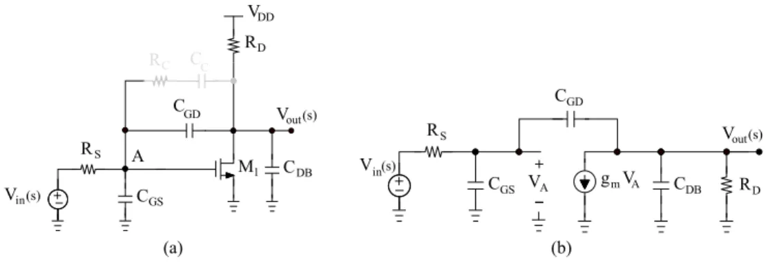
The gain of this topology is limited to the product of the input pair trans-conductance and the output impedance. In order to do the stability test, the transfer function at second stage of the two-stage op amp is considered. Figure 8 and 9 present the circuit and small signal model of a two-stage op amp with and without Miller capacitor.
Figure 8. Circuit and small signal model of second stage of op amp without Miller capacitor.
In this case, the transfer function and self-loop function of this network, which are calculated in Appendix A.3.1, are simplified as
0 1 2 0 1 2 0 1 ( ) 1 ( ) sa a H s s b sb L s s b sb
(13
)The values of given variables are
0 1 2 0 1 D GD D m D S GD DB GS GD GD D GD DB S GS GD D S m GD a R C a R g b R R C C C C C b R C C R C C R R g C (14)
In case of without frequency compensation, the transfer function of the second stage of op amp is a second-order denominator complex function. Therefore, the op amp may be stable or not. However, the two-stage op amp may prove inevitable if the output voltage swing must be maximized. Thus, the stability and compensation of this op amp are of interest.
Figure 9. Circuit and small signal model of second stage of op amp with Miller capacitor.
The transfer function and the self-loop function of this network, which are calculated in Appendix A.3.2, are simplified as
3 2 0 1 2 3 4 3 2 0 1 2 3 4 3 2 0 1 2 3 ( ) 1 ( ) s a s a sa a H s s b s b s b sb L s s b s b s b sb (15)
The values of given variables are 2 0 1 2 3 2 0 1 2 2 2 2 2 D C C GD D C C GD C m C C D GD C m C C m D D S C C GD DB GS GD DB C C D GD DB S GS GD S D GD m C C S D GS DB GD GS C GS C C C C D GD a R R C C a R R C C C g R C a R C C g R C a g R b R R R C C C C C C R C R C C R C C R R C g b R C R R C C C C C C R C R C R C C b 3 2 2 DB C D S S C C GS GD D GS DB S D GS GD DB GD DB m S D C GD C C D C D GD DB C C S GS GD C m D GD C C R R R C R C C R C C R R C C C C C g R R R C C b R R C R C C R C R C C C g R C C (16)
When the frequency compensation is considered, the transfer function of the second-stage of op amp is a fourth-order denominator complex function. It is very difficult to investigate the stable regions of this complex function. So, the measurement of the self-loop function is very important to do the stability test for the op amp.
3.2.
Stability Test for Two-Stage Op AmpIn this section, we do a stability test for the designed two-stage op amp. The op amp circuit was simulated using SPICE Spectre simulator in TSMC 0.18um CMOS process. This op amp consumes 0.25mW power from a 1.8V voltage supply. All of the circuit parameters are summarized in Table 3. Figures 10(a) and 10(b) present the models of the two-stage op amp
which can be stable and unstable. The self-loop functions in these models are measured in Figures 10(a) and 10(b). In these models, the ideal capacitors and resistors are used.
Figure 10. Models of two-stage op amp; (a) stable op amp, (b) unstable op amp; derivation of self-loop function: (c) stable case, (d) unstable case.
Table 3. Device dimension. Transistor
Size (W/L)18/0.3 1 (W/L)18/0.3 1.6/0.8 1.6/0.8 10/0.5 1.7/0.3 2 (W/L)3 (W/L)4 (W/L)5 (W/L)6 (W/L)4/0.3 7 (W/L)1/0.3 8 Capacitor
Value 0.5uF C1 0.4uF C2
Resistance
Value 3 KΩ R1 10 ΩR2
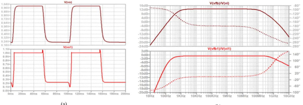
SPICE simulation results of the two-stage op amp are shown in Figure 11. Based on the voltage injection technique, the self-loop functions of two-stage op amps are measured.
In case of stable op amp, the phase margin is 100 degree at unity gain of the self-loop function. In case of unstable op amp, the phase margin is 180 degrees at near the unity gain of the self-loop function. Therefore, the damped oscillation noise makes overshoot and undershoot.
(a) (b)
Figure 11. Transient responses of two-stage op amp and simulation results of self-loop function; (brown) stable, (red) unstable.
4.
S
ECONDO
RDERL
OW-P
ASST
OWT
HOMASQ
UADRATICF
ILTERS4.1.
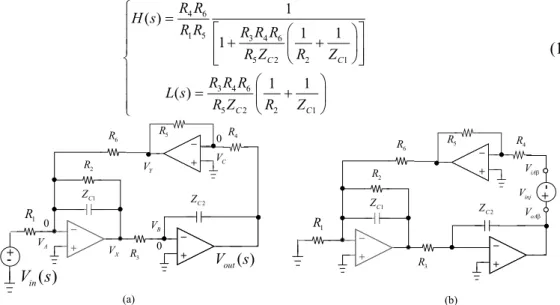
Derivation of Transfer Function and Self-Loop FunctionIn this section, the transfer function and the self-loop function of a low-pass Tow Thomas biquadratic filter are presented. This filter has been widely used because it is simple, versatile, and requires few components [12]. The Tow Thomas circuit and measurement of self-loop function are shown in Figure 12. The ideal operational amplifiers are used and the effect of the Miller’s capacitor is neglected. The transfer function and the self-loop function of this filter, which are calculated in Appendix A.4., are derived as
4 6 1 5 3 4 6 5 2 2 1 3 4 6 5 2 2 1 1 ( ) 1 1 1 1 1 ( ) C C C C R R H s R R R R R R Z R Z R R R L s R Z R Z (17) (a) (b) 1 R 3 R 2 R 6 R R5 R4 2 C Z 1 C Z +-( ) in V s Vout( )s Y V 0 0 X V 0 A V C V B V R1 3 R 2 R 6 R R5 R4 2 C Z 1 C Z Vinj oA V iA V +
-Figure 12. Analysis model (a) and derivation of self-loop function (b) for Tow Thomas circuit.
Then, Equation (17) is rewritten as
2 2 1 2 1 3 2 2 2 2 5 2 1 2 1 2 1 3 4 6 1 2 2 1 4 1 ( ) 1 2 2 2 1 2 2 R C H j R R C R R C j j R C R C R R R C C R C (18)
The stability regions of the Tow Thomas circuit are defined as
2 5 3 4 6 1 2 2 1 1 Instability 2 R R R R C C R C (19) 2 5 3 4 6 1 2 2 1 1 Marginal stability 2 R R R R C C R C (20) 2 5 3 4 6 1 2 2 1 1 Stability 2 R R R R C C R C (21)
4.2.
SPICE Simulation and Stability Test for Tow Thomas Filter
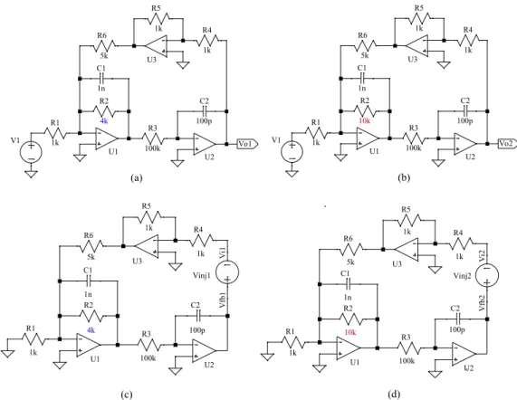
In this section, SPICE simulations are carried out using the ideal operational amplifier with the gain bandwidth (GBW) = 10MHz and DC value of open loop gain (A(s)) = 100000. The Tow Thomas circuit in Figure 13 (a) is designed for cut-off frequency f0 = 25kHz taking C1 =1 nF, C2
= 100 pF, R1= R4 = R5 = 1kΩ, R2 = 4 kΩ, R3 = 100 kΩ, and R6 = 5 kΩ. Figure 13(b) represents the Tow Thomas circuit designed with R2 = 10 kΩ and the same other values as the previous circuit. The self-loop functions of two models of the Tow Thomas circuit are shown in Figure 13(c), (d).
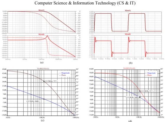
Figure 14(a) represents the SPICE simulation results of the magnitude and phase of the Tow Thomas circuit on the frequency domain. On time domain, when the pulse signals go in to these models, the transient responses are shown in Figure 14(b). The damped oscillation noise (red) occurs in case of the unstable network. The overshoot of unstable feedback system can cause extra current to flow, thereby wasting energy and cause extra heating of the components. The measurements of the self-loop functions of proposed models are shown in Figure 14(c),(d). In theoretical calculation at the half cut-off frequency 12.5 kHz (a half of f0 = 0.5 * 25 kHz = 12.5
kHz) is 63.4 degrees.
Our measurement results of self-loop functions show that
In stable case, phase margin is 72 degrees at 12.5 kHz. (> 63.4 degrees at 12.5 kHz ) In unstable case, phase margin is 51 degrees at 12.5 kHz. (< 63.4 degrees at 12.5 kHz ) The simulation results and the values of theoretical calculation are unique.
Figure 13. Models of Tow Thomas filter: (a) stable circuit, and (b) unstable circuit; derivation of self-loop function: (c) stable case, (d) unstable case.
Figure 14. Simulation results of Tow Thomas circuit: (a) frequency response, (b) transient response with square-wave input; (brown) stable, (red) unstable; frequency response of self-loop function: (c) stable, and
(d) unstable.
5.
D
ISCUSSIONThe performance of a second order low-pass filter, whether it has single-or multiple-loop control, is determined by its loop self-loop function and step input responses. These measurements show how good a second-order low-pass filter is. The self-loop function of a low-pass filter is only important if it gives some useful information about relative stability or if it helps optimize the closed-loop performance. The self-loop function can be directly calculated based on the widened superposition principle. The alternating current conservation technique (voltage injection) can measure the self-loop function of low-pass filters. Compared to the research results with mathematical analysis, the properties of self-loop functions are the same. SPICE simulation results are included. Moreover, Nyquist’s theorem shows that the polar plot of self-loop function L(s) must not encircle the point (−1, 0) clockwise as s traverses a contour around the critical region clockwise in polar chart [13]. However, Nyquist theorem is only used in theoretical analysis for feedback systems.
6.
C
ONCLUSIONSThis paper describes the approach to do the stability test for a low-pass Tow Thomas biquadradic filter. The circuitry consisting of two integrators in a feedback loop operating as a filter realizing a general biquadratic function. The transfer function of Tow Thomas circuit is a second-order denominator complex function. The term of “self-loop function” is proposed to define L(s) in a general transfer function. In order to show an example of how to define the operating region of a Tow Thomas filter, a second-order denominator complex function is analyzed. In overdamped case, the filter will amplify the high order harmonics from the first cut-off angular frequency ωcut1
to the second cut-off angular frequency ωcut2 of a step input. This causes the unwanted noise
which is called ringing or overshoot. The term of “damped oscillation noise” is proposed to define the ringing. The values of the passive components used in the Tow Thomas filter circuit
were chosen directly due to the stable conditions. All of the transfer functions were derived based on the widened superposition principle and self-loop functions were measured according to the alternating current conservation technique. The obtained results were acquired to simulations using SPICE models of the devices, including the model of a two-stage operational amplifier. In the paper not only the results of the mathematical model but also the results of simulation of the designed circuits are provided, including the stability test. The simulation results and the values of theoretical calculation of the self-loop function are unique.
A
CKNOWLEDGEMENTSForemost, we would like to express our sincere gratitude to advisor, Pro. Tanimoto (Kitami Institute. of Technology, Japan) for continuing supports.
R
EFERENCES[1] H. Kobayashi, N. Kushita, M. Tran, K. Asami, H. San, A. Kuwana, "Analog - Mixed-Signal - RF Circuits for Complex Signal Processing", IEEE 13th International Conference on ASIC (ASICON 2019) Chongqing, China (Nov, 2019).
[2] M. Tran, C. Huynh, "A Design of RF Front-End for ZigBee Receiver using Low-IF architecture with Poly-phase Filter for Image Rejection", M.S. thesis, University of Technology Ho Chi Minh City –
Vietnam, Dec. 2014.
[3] B. Razavi (2016) Design of Analog CMOS Integrated Circuits, 2nd Edition McGraw-Hill.
[4] M. Tran, Y. Sun, N. Oiwa, Y. Kobori, A. Kuwana, H. Kobayashi, "Mathematical Analysis and Design of Parallel RLC Network in Step-down Switching Power Conversion System", Proceedings of International Conference on Technology and Social Science ICTSS 2019, Kiryu, Japan (May. 2019).
[5] M. Tran, N. Kushita, A. Kuwana, H. Kobayashi, "Flat Pass-Band Method with Two RC Band-Stop Filters for 4-Stage Passive RC Quadratic Filter in Low-IF Receiver Systems", IEEE 13th International Conference on ASIC (ASICON 2019) Chongqing, China (Nov. 2019).
[6] M. Tran, Y. Sun, Y. Kobori, A. Kuwana, H. Kobayashi, "Overshoot Cancelation Based on Balanced Charge-Discharge Time Condition for Buck Converter in Mobile Applications", IEEE 13th International Conference on ASIC (ASICON 2019) Chongqing, China (Nov. 2019).
[7] R. Schaumann and M. Valkenberg (2001) Design of Analog Filters, Oxford University Press.
[8] R. Middlebrook, "Measurement of Self-Loop function in Feedback Systems", Int. J. Electronics, Vol 38, No. 4, pp. 485-512, 1975.
[9] A. Sedra, K. Smith (2010) Microelectronic Circuits, 6th ed. Oxford University Press, New York. [10] M. Tran, "Damped Oscillation Noise Test for Feedback Circuit Based on Comparison Measurement
Technique", 73rd System LSI Joint Seminar, Tokyo Institute of Technology, Tokyo, Japan (Oct. 2019).
[11] H. Kobayashi, M. Tran, K. Asami, A. Kuwana, H. San, "Complex Signal Processing in Analog, Mixed - Signal Circuits", Proceedings of International Conference on Technology and Social Science 2019, Kiryu, Japan (May. 2019).
[12] J. Tow, "Active RC Filters-State-Space Realization", IEEE Proceedings, Vol. 56, no. 6, pp. 1137–
1139, 1968.
[13] J. Wang, G. Adhikari, N. Tsukiji, M. Hirano, H. Kobayashi, K. Kurihara, A. Nagahama, I. Noda, K. Yoshii, "Equivalence Between Nyquist and Routh-Hurwitz Stability Criteria for Operational Amplifier Design", IEEE International Symposium on Intelligent Signal Processing and Communication Systems (ISPACS), Xiamen, China (Nov. 2017).
A
PPENDIXA.1. Second order denominator complex function From Equation (1), the transfer function is rewritten as
2 2 2 2 1 1 ( ) 2 2 2 2 a H s as bs c b b c b s s a a a a (22) The simplified form of Equation (22) is
2 2 2 2 2 2 2 2 2 4 4 ( ) 2 2 2 2 2 2 1 1 2 2 a a b b H s a a a c b a a c b s s s b b b a a b b a a (23) In the form of angular frequency variable, the transfer function is
2 2 2 2 4 ( ) 2 2 1 2 a b H j a a c b j b b a a (24)
In critically damped case: 2
2 c b a a
,
Equation (24) is simplified as 2 2 2 arctan 2 arctan 2 2 2 2 2 2 4 1 4 4 ( ) 2 2 2 1 1 1 a a j j b b a a e a e H s b a b a b a j b b b (25)Here, the cut-off angular frequency is
2
cut b
a
. At the cut-off angular frequency, the
magnitude and phase of the transfer function are
2 ( ) 2 2 2 ( ) 2 ( ) ( ) 2 j j H s a H s a b H s e e b H s (26) In underdamped case: 2 2 c b a a
,
let us define 2 2 2 2 2 c b c b a a a a , then Equation (24) is rewritten as 2 2 2 2 2 2 2 4 4 ( ) 2 2 2 2 2 2 1 1 1 2 2 2 a a b b H s a c b a a c b a a a c b j j j b a a b b a a b b b a a (27) Now, the transfer function is rewritten as2 2 2 2 arctan arctan 2 2 1 1 2 2 2 2 2 2 2 4 ( ) 2 2 2 1 1 2 2 a a b b j j a c b a c b b a a b a a a e e H j b a c b a a c b b a a b b a a 2 2 2a b (28)
The cut-off angular frequencies are 2 1 2 1 2 2 cut b a c b a b a a
and
2 2 2 1 2 2 cut b a c b a b a a In overdamped case: 2 2 c b a a,
let us define 2 2 2 2 2 c b c b j a a a a , then Equation (24) is rewritten as 2 2 2 2 2 2 2 4 4 ( ) 2 2 2 2 1 1 1 2 2 2 a a b b H s a c b a c b a a c b j j j j b a a b a a b b a a (29) Now, the transfer function is rewritten as2 2 2 2 arctan arctan 2 2 2 2 2 2 2 4 ( ) 2 2 1 1 2 2 a c b a c b j j b a a b a a a e e H j b a c b a c b b a a b a a (30)
The cut-off angular frequencies are 2
1 2 1 2 2 cut b a c b a b a a
and
2 2 2 1 2 2 cut b a c b a b a a.
A.2. Self-loop function of second order denominator complex function From Equation (7), the self-loop function is rewritten as
2 2 2 4 2 2 ( ) 2 a a a c b L j j j b b b a a (31)
In critically damped case: 2
2
c b
a a , the self-loop function is
2 arctan 4 4 ( ) 1 1 b j a a a a a L j j j e b b b b (32)
The cut-off angular frequencies of the self-loop functions are 1 0 and 2 b
a. At unity gain of the self-loop function, we have
2 4 ( u) 1 u 1 u 1 a a L b b (33)
Solving Equation (33), the angular frequency u at unity gain is calculated as
5 2 2
u b
a (34)
The relationship between the angular frequency uand the cut-off angular frequency
2 cut b ais 5 2 5 2 u u cut cut (35)
A.3. Small signal models of second stage of op amp
A.3.1 Second stage of op amp without Miller’s capacitor
Figure 15. Circuit of Figure 8(b).
Apply the widened superposition at VA node, we get
1 1 1 in out A S CGS CGD S CGD V V V R Z Z R Z (36)
Then, apply the widened superposition at Vout node, we get
1 1 1 1
out A m
CGD CDB D CGD
V V g
Z Z R Z (37)
The voltage VA is simplified as
1 1 1 1 1 A out CGD CDB D m CGD V V Z Z R g Z (38) The transfer function of this network is
1 ( ) 1 1 1 1 1 1 1 1 1 1 1 1 m CGD S m CGD CDB D CGS CGD CGD CDB D CGD CGD GD m GD DB S GS GD GD DB GD m GD D D g Z H s R g Z Z R Z Z Z Z R Z Z sC g sC sC R sC sC sC sC sC g sC R R (39)
Now, the simplified transfer function of this network is
2 2 ( ) 1 D GD D m D S GD DB GS GD GD D GD DB S GS GD D S m GD sR C R g H s s R R C C C C C s R C C R C C R R g C (40)
A.3.2. Second stage of op amp with Miller capacitor
Figure 16. Circuit of Figure 9(b).
Apply the widened superposition at VA node, we get
1 1 1 1 in 1 1 A out S CGS CGD C CC S CGD C CC V V V R Z Z R Z R Z R Z (41)
Then, apply the widened superposition at Vout node, we get 1 1 1 1 1 1 out A m CGD C CC CDB D CGD C CC V V g Z R Z Z R Z R Z (42)
The transfer function of this network is
1 1 ( ) 1 1 1 1 1 1 1 1 1 1 1 1 1 1 1 1 m CGD C CC CGD C CC CDB D CGS CGD C CC S CGD C CC CDB D m CGD C CC CGD C CC C GD m C C GD g Z R Z H s Z R Z Z R Z Z R Z R Z R Z Z R g Z R Z Z R Z sC sC g sR C s sC 1 1 1 1 1 1 1 C C GD DB GS GD C C D C C C DB S C C D C C GD m GD C C C C sC sC sC sC sC sC sR C R sR C C sC R sR C R sC sC sC g sC sR C sR C (43)
Now, the simplified transfer function of this network is 2 3 2 2 4 3 2 2 2 ( ) 2 2 D C C GD D C C GD C m C C D GD C m C C m D D S C C GD DB GS GD DB C C D GD DB S GS GD S D GD m C C S D GS DB GD GS C GS C C C C s R R C C s R R C C C g R C sR C C g R C g R H s s R R R C C C C C C R C R C C R C C R R C g s R C R R C C C C C C R C R C s 2 2 1 D GD DB C D S S C C GS GD D GS DB S D GS GD DB GD DB m S D C GD C C D C D GD DB C C S GS GD C m D GD C R C C C R R R C R C C R C C R R C C C C C g R R R C C s R R C R C C R C R C C C g R C C (44)
A.4. Low-pass Tow Thomas biquadratic filter
1 R 3 R 2 R 6 R R5 R4 2 C Z 1 C Z + -( ) in V s Vout( )s Y V 0 0 X V 0 A V C V B V
Figure 17. Circuit of low-pass Tow Thomas biquaratic filter.
1 2 1 6 1 1 0 in Y X C V V V R R Z R (45)
Do the same work at node VB, we get
3 3 2 2 0 out X X out C C V R V V V R Z Z (46)
Then at node VC, we get
5 4 5 4 0 out Y Y out V V R V V R R R (47)
The transfer function of this filter is derived as
4 6 1 5 3 4 6 5 2 2 1 1 3 1 2 2 5 2 1 3 4 6 1 2 1 ( ) 1 1 1 1 1 1 out in C C V R R H s V R R R R R R Z R Z R R C C R s s R C R R R C C (48)
A
UTHORSMinh Tri Tran received the B.S. and M.S. degree from the University of Technical Education Ho Chi Minh City (HCMUTE) – Vietnam, and University of Technology Ho Chi Minh City (HCMUT) – Vietnam, in 2011, and 2014, respectively, all in Electrical and Electronic Engineering. He joined the Division of Electronics and Informatics, Gunma University, Japan in 2018, where he is presently working toward the Ph.D. degree in
Electrical and Electronic Engineering. His research interests include modelling, analysis, and test of damped oscillation noise and radio-frequency radiation noise in communication systems.
Anna Kuwana received the B.S. and M.S. degrees in information science from Ochanomizu University in 2006 and 2007 respectively. She joined Ochanomizu University as a technical staff, and received the Ph.D. degree by thesis only in 2011. She joined Gunma University and presently is an assistant professor in Division of Electronics and Informatics there. Her research interests include computational fluid dynamics.
Haruo Kobayashi received the B.S. and M.S. degrees in information physics from University of Tokyo in 1980 and 1982 respectively, the M.S. degree in electrical engineering from University of California, Los Angeles (UCLA) in 1989, and the Ph. D. degree in electrical engineering from Waseda University in 1995. In 1997, he joined Gunma University and presently is a Professor in Division of Electronics and Informatics there. His research interests include mixed-signal integrated circuit design & testing, and signal processing algorithms.
© 2020 By AIRCC Publishing Corporation. This article is published under the Creative Commons Attribution (CC BY) license.