M E T H O D O L O G Y A R T I C L E
Open Access
Improved high-dimensional prediction
with Random Forests by the use of co-data
Dennis E. te Beest
1, Steven W. Mes
3, Saskia M. Wilting
4, Ruud H. Brakenhoff
3and Mark A. van de Wiel
1,2*Abstract
Background: Prediction in high dimensional settings is difficult due to the large number of variables relative to the sample size. We demonstrate how auxiliary ‘co-data’ can be used to improve the performance of a Random Forest in such a setting.
Results: Co-data are incorporated in the Random Forest by replacing the uniform sampling probabilities that are used to draw candidate variables by co-data moderated sampling probabilities. Co-data here are defined as any type information that is available on the variables of the primary data, but does not use its response labels. These
moderated sampling probabilities are, inspired by empirical Bayes, learned from the data at hand. We demonstrate the co-data moderated Random Forest (CoRF) with two examples. In the first example we aim to predict the presence of a lymph node metastasis with gene expression data. We demonstrate how a set of externalp-values, a gene signature, and the correlation between gene expression and DNA copy number can improve the predictive performance. In the second example we demonstrate how the prediction of cervical (pre-)cancer with methylation data can be improved by including the location of the probe relative to the known CpG islands, the number of CpG sites targeted by a probe, and a set ofp-values from a related study.
Conclusion: The proposed method is able to utilize auxiliary co-data to improve the performance of a Random Forest. Keywords: Classification, Random forest, Gene expression, Methylation, DNA copy number, Prior information
Background
High-dimensional prediction is inherently a difficult prob-lem. In this paper we demonstrate how to improve the per-formance of the Random Forest (RF) on high-dimensional (in particular genomics) data by guiding it with ‘co-data’. Here, co-data is defined as any type of qualitative or quan-titative information on the variables that does not use the response labels of the primary data. The primary data may, for example, be a set of gene expression profiles with corresponding binary response labels. Examples of co-data are:p-values on the same genes in a external, related study, correlations with methylation or DNA copy number data, or simply the location on the genome. Guiding a pre-diction model by co-data may lead to improved predictive performance and variable selection.
*Correspondence: [email protected]
1Department of Epidemiology and Biostatistics, VU University Medical Center,
1007 MB Amsterdam, The Netherlands
2Department of Mathematics, VU University, 1081 HV Amsterdam, The
Netherlands
Full list of author information is available at the end of the article
Several methods are able to incorporate co-data dur-ing model traindur-ing. A general multi-penalty approach was suggested by [1], a weighted lasso by [2], and a group-regularized ridge by [3]. These methods are all based on penalized regression, with a penalty parameter that is allowed to vary depending on the co-data, effec-tively rendering co-data based weights. The group-lasso [4] and sparse group-lasso [5] are also regression-based, but these methods apply a specific group-penalty that can exclude entire groups of variables. Except for the group-regularized ridge, all these methods allow for only one type of co-data. In addition, except for the weighted lasso, these methods require the co-data to be specified as groups. The weighted lasso can handle one source of continuous co-data, but requires an assumption about the functional form of the penalty weighting and the co-data. For some types of co-data this functional form is largely unknown. Hence, it may be desirable to learn it from the co-data, and to enforce monotonous weights to ensure stability and interpretability.
© The Author(s). 2017Open AccessThis article is distributed under the terms of the Creative Commons Attribution 4.0 International License (http://creativecommons.org/licenses/by/4.0/), which permits unrestricted use, distribution, and reproduction in any medium, provided you give appropriate credit to the original author(s) and the source, provide a link to the Creative Commons license, and indicate if changes were made. The Creative Commons Public Domain Dedication waiver (http://creativecommons.org/publicdomain/zero/1.0/) applies to the data made available in this article, unless otherwise stated.
The Random Forest (RF) is a learner that is popular due to its robustness to various types of data inputs, its abil-ity to seamlessly handle non-linearities, its invariance to data transformations, and its ease of use without any or much tuning [6]. The RF is suitable and computationally efficient for genomics data, with typically the number of variables, P, largely exceeding the sample size, n [7, 8]. Its scale invariance makes it a good candidate to analyse RNASeq data. Due to the skewed nature of such data, their analysis is less straightforward with penalized regression techniques and results depend strongly on the data trans-formation applied [9]. Our aim is to develop a co-data moderated RF (CoRF) which allows the joint use of mul-tiple types of co-data, the use of continuous co-data, and flexible modeling of the co-data weights. Conveniently, these co-data are only used when training the classifier; they are not required for applying the classifier to new samples.
The described methodology can in principle be used with any bagging classifier that uses the random subspace method [10], but in this paper we focus on the RF. The method is exemplified with two examples. First, we aim to predict the presence of a lymph node metastasis (LNM) for patients with head and neck squamous cell carci-noma (HNSCC) using TCGA RNAseq data. We show how the use of several types of co-data, including DNA copy number, an external gene signature and mRNA microar-ray data from an independent patient cohort, improves the predictive performance, and validate these results on a second independent data set. The computational effi-ciency of the method is illustrated with a second example, where our aim is to predict the last precursor stage for cervical cancer based on methylation data with very large P ≈ 350.000. The co-data in this example consists of the location of the methylation site, the number of CpGs, and the external set ofp-values.
Methods and Results
Random forest
The aim of a supervised RF is to predict per sample i,i = 1,. . .,n, an outcomeYiusing a set of variablesXij
wherej=1,. . .,Pindicates the variables. Here, we focus on binary outcomeYi, although the entire methodology
and software also applies to continuous and censored (e.g. survival) outcomes. A RF consists of a large number of unpruned decision trees, where each tree is grown on a bootstrap sample of the data. At each node split in each tree only a random subset of the variables are candidates, its size denoted bymtry, typically set at√P. In a standard RF, all variables have an equal probability of being candi-dates. Predictions are issued by majority voting across all trees, or on a fractional scale (fraction of trees predicting Yi=1). We will use the latter for assessing predictive
per-formance. A RF is fitted to a bootstrap sample of the data
implying that per tree the remaining fraction (on aver-age 0.368) is out-of-bag (oob) and can be used to obtain an estimate of the prediction error. This leads to a com-putational advantage compared to methods that require cross-validation for this purpose.
Group-specific probabilities
We first briefly describe our method using one source of grouped co-data only. Here, the basic idea is that, when an a priori grouping of variables is available (co-data), we may sample the variables according to group-specific probabil-ities, and these probabilities can be estimated empirically from the data. When the number of groups is limited, only a few parameters need to be estimated (the group specific probabilities). Especially when the difference in predictive power between groups of variables is large, the predictive performance may be enhanced.
In practice, this means we first need to run a base RF (i.e. uniform sampling probabilities). From this initial fit, we obtain the number of times each variable is used across all trees. Then, the new group-specific probabilitieswgare:
wg= ˆ pselg −γp0 + , (1)
where pˆselg is the proportion of selected variables from groupgacross all trees divided by the size of groupgand p0 = 1/P is the expected value ofpˆselg when the group structure is uninformative. Parameter γ can be used to tune the RF to adapt to group-sparsity by thresholding, but may also be set to one to avoid tuning. After nor-malizingwg such that these sum to one across variables,
we obtain sampling probabilities w˜g. Then, a new RF is
trained using these probabilities instead of the uniform ones, rendering the CoRF.
Model-based probabilities
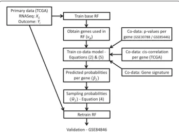
Next we extend the described method to allow for mul-tiple sources of co-data, including continuous co-data. Figure 1 schematically displays the method for the first application. First, we enumerate all node splits in all trees. Then, we definevjk as a binary variable indicating
whether or not variable jwas used in thekth split, and Vj = kvjk as the total number of times that variablej
was used.
The main challenge in modeling multiple types of co-data, is that the various types of co-data may be collinear. We therefore need to de-tangle how well the various types of co-data explainvjk. For that, we use a co-data model. We
propose to use the logistic regression framework for this. We denote theP×Cco-data design matrix byX, where Xjc contains the co-data information for thejth variable
and thecth co-data type, and where nominal co-data on Llevels is represented byL−1 binary co-data variables.
Fig. 1Illustration of the sources of data used in CoRF for the LNM example. First, a base RF is fitted on the training data. Its output,vij, together with the co-data, is used to train the co-data model. From the co-data model, we obtain a probability per gene used for refitting on the training data. In an extra step we validate the results on GSE84846
Then,vjkis Bernoulli distributed withvjk∼Bern(pj), and
we estimatepjusing a logistic regression:
logit(pj)=α0+ C
c=1
Xjcαc (2)
From the co-data model, we obtain a predicted probabil-ity per variable,pˆj. Note that inclusion of the interceptα0
in (2) guarantees thatPj=1pˆj=1, as desired. The logistic
regression establishes a marginal relationship betweenvjk
andXjc. For modelingVj, first note thatvjk contains two
types of dependencies: (1) a dependency between splitsk for a given variablej, e.g. only one variable can be chosen per split; (2) dependency between variables and therefore, between their selection frequencies (Vj). The first
depen-dency is addressed by using a quasi-binomial likelihood qBin(Vj;α,τ)forVj = kvjk, which allows for an
over-or under-dispersion parameterτ by modeling Var(Vj) =
τpj(1−pj)[11]. We do not explicitly address the second
type of dependency, which implies that the estimation is based on a pseudo-log-likelihood: ˆ α,τˆ=max α,τ ⎡ ⎣P j=1 logqBinVj;α,τ ⎤⎦ . (3)
As a result the uncertainties of the estimates and the p-values of the co-data model do not have a classical inter-pretation, and cannot directly be used for inference. We are, however, primarily interested in the point estimates, ˆ
pj, obtained by substitutingαˆ into (2), which are used to
re-weigh variables:
wj=pˆj−γp0+. (4)
As earlier,γ can be set to 1 which provides a natural cut-off forp0, orγ may be tuned to more or less sparsity. Finally, we normalize wj to obtain the sampling
proba-bilitiesw˜j = wj/jwj, which are then used to re-train
the RF.
The relationships we are interested in are often non-linear, e.g. for external p-values the difference between 10−4 and 10−2may be more relevant than that between 0.25 and 0.50. We therefore extend the linear model (2) to include more flexible modeling of continuous co-data with a monotonous effect, which is often natural and desirable. For that, we fit a generalized additive model with a shape constrained P-spline (SCOP, [12]), as imple-mented in the Rpackage scam. Then, Eq. (2) becomes
logit(pj)=α0+ C1 c=1 Xjcnαc+ C2 d=1 fd Xjdc (5) whereXn(Xc) denotes the sub-matrix ofXcontaining the nominal (continuous) co-data, andfd()represents a
flex-ible function provided by the SCOP. To modelfd, SCOP
usesm(x) = q=1θB(x), where Bis a B-spline basis function, which is monotonously increasing whenθ ≥
θ−1,= 1,. . .,q[12]. The monotony inθ is enforced by
definingθ = θ˜, whereθ˜ =[θ˜1, exp(θ˜2),. . ., , exp(θ˜q)]T
andrs = 0 if r < s andrs = 1 if r s.
Smooth-ness is enforced by penalisation of the squared differences analogous to [13]. Settingrs = −1 forr srenders a
monotonically decreasing spline. Unrestricted splines can in principle also be used in the co-data model, but are more liable to over-fitting.
Instead of using the default ofγ = 1, this parameter can be tuned by a grid search. This requires calculatingwj
and refitting a RF for each grid-value ofγ. The optimal value ofγ is then the one with the best oob performance. Note that tuningγ with the oob predictions may result in a degree of optimism. This may be solved by embedding the procedure in a cross-validation loop. Whenγ is not tuned, the oob performance of CoRF may also be slightly optimistic, because the primary data was used to estimate the weights (4). However, when the regression model (2) is parsimonious, the overoptimism is likely small, as veri-fied empirically in the Application section. To ensure that the co-data model is parsimonious, it may be useful to perform co-data selection to remove redundant co-data sources, which also assists in assessing the relevance of the co-data. The Additional file 1 supplies an heuristic procedure to do so.
CoRF algorithm
The CoRF procedure may by summarized as follows:
1. Fit a base RF with uniform sampling probabilities and obtainvjk.
2. To disentangle the contributions of the various co-data sources.
• Fit co-data model (2), if only linear effects are assumed.
• Fit co-data model (5) with shape constrained
P-spline(s), if flexible, monotone effects are required.
• Optionally: exclude redundant co-data sources
and re-fit the co-data model.
3. Obtain the predicted probabilitiespˆjfrom the fitted
co-data model.
4. Calculate the sampling probabilitieswjwith
threshold parameterγ. Default is to setγ =1, optionallyγ can be tuned.
5. Refit the RF for each vector ofw˜j.
6. • Ifγ is not tuned (i.e.γ = 1), we directly obtain the CoRF, the base RF and their oob
performances.
• Ifγ is tuned, obtainγˆby maximizing the oob
performance. Tuningγ may introduce a bias in
the oob performance. Hence, the entire procedure is cross-validated whenγ-tuning is employed.
Implementation
The method as described here is implemented in a corresponding R package, called CoRF, and is available on GitHub. It depends on the R package
randomForestSRCfor fitting the RF [14–16]. A feature of this package that is of key importance for CoRF is the option to assign a sampling probability per variable. In addition, randomForestSRC applies to regression, classification and survival analysis, and by extension, so does CoRF.
For classification by the RF the recommended mini-mal node size is one. The node size can be tuned [17], but a RF is not very sensitive to the minimal node size. In CoRF the quality of the selected variables may influ-ence the fit of the co-data model. Variables that are used higher up in a tree are, on average, more relevant, and variables that split a node of size 2 are the least relevant. For CoRF, we believe it is better to slightly increase the minimal node size, improving the quality of the selected variables and as a result improve the quality of the co-data model. As default in CoRF, we set the minimal node size for classification at 2.
Generally, CoRF will need a larger number of trees to fit than a base RF. A base RF needs enough trees to capture the underlying signal in the data. CoRF additionally needs an indication of the relevance of each variable, which feeds back to the co-data model. Also, a co-data model that con-tains splines generally needs more trees than a co-data
model with only linear effects. In the LNM example, described below, we set the number of trees at 15.000 to ensure convergence of both the RF/CoRF and the co-data model. A lower number of trees, e.g. 2.000, gives a similar result in terms of predictive performance, but the variabil-ity between fits increases. When using CoRF, we recom-mend to use at least 5.000 trees to ensure a reliable, good fit of the co-data model. An additional advantage of a large number of trees with tuning is that the variability between RF fits decreases, allowing for a more reliably selection ofγ.
A RF is a computationally efficient algorithm to use for high dimensional data, primarily because at each node it selects only from √P variables. CoRF inherits this effi-ciency and when the defaultγ = 1 is used, only one RF refit is needed. Next to (re)fitting the RF, the only addi-tional computation required for CoRF consists of fitting the co-data model. Further tuning ofγ may improve the performance, but also requires i) refitting a RF for each value for γ, and ii) an additional cross-validation loop to assess performance, thereby increasing computational cost considerably.
Evaluating predictive performance
The predictive performance of CoRF and other classi-fiers was assessed on oob samples by two metrics: i) the area-under-the-roc curve (AUC; [18]); and ii) the Brier score [19]. AUC is based on ranks and evaluates discrim-ination. It combines sensitivity and specificity, which are both important in a clinical setting. Moreover, it is a good indicator for the performance of a RF with unbalanced data [18]. Brier score is based on residuals and evalu-atescalibration. It equals the average Brier residual, i.e. Bi = (Yi−qi)2, whereqi is the fraction of trees
predict-ingYi=1. Brier score is reported in a relative sense, with
the base RF as benchmark. For comparing CoRF with RF we implemented significance testing, both forAUC: the difference between AUCs, using R’s pROC package [20] and forBrier: the difference between Brier scores, using the one-sided Wilcoxon signed-rank test on paired Brier residualsBRFi ,BCoRFi . When performance was evaluated on the same data as used for training, we used multiple 2/3 - 1/3 splits, meaning that the power for testing, for which only 1/3 of the samples can be used, can be limited. These splits result in multiplep-values, which we aggregate by applying the median, which was proven to control the type I error rate under mild conditions [21].
Similarly to the base RF, CoRF automatically renders oob predictions. CoRF is an empirical Bayes-type classi-fier, which uses the relation between the co-data and the primary data to estimate sampling weights. Such double use of data could lead so some degree over overopti-mism, although this will likely be limited given that the co-data model is parsimonious. In addition, when splines
were used, the effective degrees-of-freedom were reduced by imposing monotony. Nevertheless, in the examples below, we verified the oob performance of CoRF by cross-validation when training and evaluation was applied on the same data.
Comparable methods
To our knowledge, there is only one high-dimensional pre-diction method that can explicitly takemultiple sources of co-data into account: the group-regularized (logistic) ridge (GRridge[3]). CoRF provides several conceptual advantages over GRridge. First, unlike CoRF, GRridge requires discretisation of continuous co-data. Second, CoRF fits the co-data coefficients in one model, (2), instead of using the co-data sources iteratively. Third, CoRF is computationally more efficient, because it a) inherits the better computational scalability of RF with respect toP; and b) requires very little tuning and no iter-ations. Finally, as with a base RF, CoRF is naturally able to incorporate categorical outcomes with>2 groups (as demonstrated in the cervical cancer example). GRridge inherits the advantages of ridge regression, e.g. better interpretability of the model and the ability to include mandatory covariates. In the Application section we com-pare the performances of these two methods for the LNM example.
Applications
Predicting Lymph node metastasis with TCGA data To exemplify the CoRF method, we use it to predict the presence of a lymph node metastasis (LNM) for patients with HPV negative oral cancer using RNASeqv2 data from TCGA [22]. We focus on the HPV-negatives, because these constitute the majority (approx. 90%) of the oral cancers, and HPV-positive tumors are known to have a different genomic etiology [23]. Early detection of LNM is important for assigning the appropriate treatment. Diag-nosis of LNM with genomic markers could potentially improve diagnosis and treatment [24].
The primary data consists of normalized TCGA RNASeqv2 profiles of head-and-neck squamous cell carci-nomas (HNSCC), which were downloaded together with the matching normalized DNA copy number co-data from Broad GDAC Firehose using the R packageTCGA2STAT. Of the 279 patients described in [22], we used the sub-set of 133 patients that had HPV-negative tumors in the oral cavity. Of these patients, 76 presented a LNM and 57 did not.
To enhance the prediction of the base RF, we consider three types of co-data in this example: (1) DNA copy number; (2) p-values from the external microarray data GSE30788/GSE85446; (3) a previously identified gene sig-nature [24–26]. These three types of co-data demonstrate the variety of co-data sources that can be included in
CoRF. The DNA copy number data are measurements on the same patients. We use the cis-correlations between DNA copy number and the RNASeqv2 data. Given the nature of RNASeqv2 and DNA copy number data (dis-crete and ordinal, respectively), we applied Kendall’sτ to calculate the correlations, giving τj,j = 1,. . .,P. Note
that the DNA data are only used during training of the predictor; these arenot required for test samples, which distinguishes this type of predictor from integrative pre-dictors [27]. The p-values of GSE30788/GSE85446 are derived from measurements of the same type of genomics features (mRNA gene expression), but measured on a different platform (microarray) than that of the primary RNAseq data and on a different set of patients. The gene signature is a published set of genes that were found to be important in a different study. Figure 1 illustrates how the various types of data are used within CoRF.
Each type of co-data has its own characteristics that needs to be taken into account in the co-data model. For the DNA copy number data, we a priori expect that a gene with a positive cis-correlation is more likely to be of importance to the tumor [28]. We use a monotonically increasing splinef1to model the relation betweenpjand Xcj1 = τj (5). For the p-values of GSE30788/GSE85446,
we a priori expect that genes with a lowp-value are more likely to be important on the TCGA data, and we thus use a monotonically decreasing splinef2to model the relation
betweenpjandXj2c =pvalj. The third type of co-data,
con-sisting of the published gene signature is included in the co-data model (2) as a binary variable:Xj1n =1 when gene jis part of the signature, and 0 otherwise.
Data set GSE30788/GSE85446 consists of 150 Dutch patients (of which 60 presented a LNM and 90 did not) with a HPV-negative oral cancer tumor who are in that respect similar to the TCGA patients. Gene expression was measured by microarray, thep-values on GSE30788/ GSE85446 were calculated using a Welch two-sample t-test; further details on the study can be found in [29]. The differences between the TCGA and the Dutch data (notably the platform and the geographical location of the patients) preclude a straightforward meta-analytic data integration. Also, our focus here is on the TCGA data, which were measured on a more modern platform, but shared genomic features with the Dutch co-data may enhance the weighted predictions.
After training the base RF and the CoRF, we validate these classifiers on an independent data set (GSE84846). GSE84846 contains microarray expression data of 97 HPV-negative oral cancer patients from Italy, of whom 49 had a LNM [29]. To directly apply the classifiers to the validation data, we need to account for the differ-ences in scale between RNASeqv2 and microarray data. First, the TCGA RNASeqv2 data are transformed by the Anscombe transformation (i.e.√(x+ 3/8)). Next, both
the TCGA RNASeqv2 and GSE84846 data are scaled to have zero mean and unit variance. We only included genes that could uniquely be matched between the two data sets (leaving 12838 genes). Since this validation does not require any re-training, the performance is directly assessed by comparing the predictions with the actual labels. As an alternative to this validation, we also use the relative frequency of variables used by the base RF and CoRF on the TCGA data as sampling probabilities in training a new RF on GSE84846 data, in which case the oob-performance was used.
We also assess the performance of the base RF and CoRF in terms of variable selection on both the train-ing and validation data sets. For the TCGA traintrain-ing data set, we first select a set of genes (based on Vj), retrain
on this subset, and assess the performance with a 10-fold cross-validation. For the validation data set, we first select variables on the TCGA training data with the variable-hunt-vimp (vh-vimp) as described by [30]. Roughly, vimp measures the importance of a variable by assessing the decrease in predictive performance when the values of the variable are ‘noised up’, e.g. randomly permuted across samples. Then, we refit with the selected set of variables on the TCGA training data, and evaluate the performance of the refitted model on the validation data using oob-performance. To assess the stability of variable selection with a base RF and CoRF, we repeatedly (20 times) sam-ple 84 out of 133 TCGA cases without replacement and fit a base RF and CoRF to each sampled set. Note that the sampling fraction mimics the expected fraction of independent samples in a re-sampling scheme, 0.632. We preferred subsampling over resampling here, because the latter would lead to duplicate samples in the sampled set. Stability of gene selection was then assessed by calculating the average overlap between any combination of two sets of variables selected from the subsampled training sets, varying the sizes of the selection sets from 10, 20,. . ., 100 genes.
Performance on LNM example
By examining the fit of the co-data model (Fig. 2), we observe that pˆj is estimated higher for genes with a
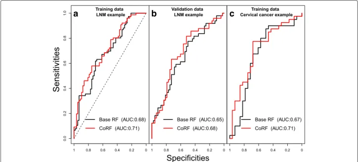
high cis-correlation, for genes with a low p-value on GSE30788/GSE85446, and for genes that are present in the gene signature. By prioritising these genes we observe an improvement in oob-AUC (base RF: 0.682, CoRF: 0.706) and a relative decrease in oob-Brier score of 2.7%. Figure 3a and b show the ROC-curves (specificity versus sensitivity), parametrized by a threshold for the propor-tion of trees predicting LNM. When assessing significance using ten 2/3 - 1/3 splits, rendering an effective test sam-ple size ofntest = n/3 ≈ 44, the median p-values equal
˜
pAUC = 0.255 and p˜Brier = 0.034, hence significant
at α = 0.05 for the latter. In terms of Brier residuals,
predictions improved for 27.2 out of 44 test samples, on average across splits. With 10-fold cross-validation we also see an improvement by using CoRF (cv-AUC base RF: 0.675, CoRF: 0.690). On the validation data we find that CoRF renders a slightly larger improvement (AUC base RF: 0.652, CoRF: 0.682); here the Brier score decreases by 2.6%. In this case we may use all 97 samples for signifi-cance testing. Then, the resultingp-values are:pAUC =
0.056 and pBrier = 0.0048, hence close to significant
for the first and significant for the latter metric. In terms of Brier residuals, predictions improved for 64 out of 97 samples.
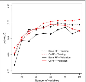
Retraining on the validation data using only the sam-pling probabilities derived from either the base RF/CoRF fits to the TCGA data yields a similar result (oob-AUC base-RF: 0.656, CoRF: 0.695). From Fig. 4 we observe that CoRF also improves the oob-AUC when applying variable selection to both the training and validation data. Finally, stability of gene selection, when selecting genes with the vh-vimp measure, increased by 17%, averaged across sizes of the selection sets. This means that when selecting genes using random subsets of samples the overlap between two selected sets of equal size is on average substantially higher with CoRF than with RF. For gene selection with Vjthe average stability increased by 36%. For these data,
tuning ofγdoes not improve results, see Additional file 1. For comparison with GRridge, we find a cv-AUC of 0.682 on the training data and AUC of 0.689 on the val-idation data. With GRridge the global penalty parameter of the ridge regression was estimated using a 10-fold cross-validation and performance on the training data was assessed using a second 10-fold cross-validation. For the validation data we directly applied the resulting classi-fier. In performance this is comparable to CoRF, but note that CoRF is quicker, especially when we want an estimate of the prediction error (see the “Computational time” section).
Cervical cancer example
In this second example, our aim is to predict cervical (pre-)cancer on a very high-dimensional methylation data set. The methylation data consists of 365620 methylation sites, and contains 68 samples of which 28 correspond to normal cervical tissue, 36 have a high-grade precur-sor lesion (CIN3; CIN = cervical intraepithelial neoplasia) and 4 have cervical cancer. A diagnosis of either of the lat-ter two stages usually implies surgery. The samples were taken using a self-sample test, implying a challenging diag-nostic setting. The data used in this example originate from [31] where more information can be found on the clinical details and on the preprocessing of the methyla-tion data. When training the RF, we consider the three separate categories, while for the final prediction we add up the votes for CIN3 and cancer, because of the small
a
b
Fig. 2Fit of the co-data model for the LNM example. Each square represents 100 genes grouped by either (a) DNA copy number-expression correlation or (b)p-value. The red lines represent the marginal fit across the correlations orp-values. The top red lines represent the fit for genes present in the gene profile. The cloud of red dots represent the fitted values for 1000 randomly selected genes
sample size for the latter. As before, our aim is to improve the prediction of the base RF by including co-data (e.g. CoRF).
The co-data consists of the location of the probe rela-tive to the known CpG islands (categorized in 6 classes, including CpG-island), the number of CpG sites included in the genomic location targeted by the probe, and p-values, obtained by differential methylation analysis on a related, external study [32]. The latter study also com-pares methylation levels of normal cervical tissue (20) versus CIN3’s (17), but on surgically obtained cervical tis-sue. Hence, the setting is different than for our primary self-sample study, but these co-data are possibly very use-ful. The location of the probe is modeled as a nominal variable in the co-data model. From the fit of the co-data
model (Fig. 5), we observe that the location of probe has as strong effect onpˆj, and indeed CpGs located within a CpG
island are most important. The number of CpG sites can be either modeled as a factor variable or with a monoton-ically increasing spline. We opted for the second option, thus explicitly assuming that methylation sites with more CpG sites are likely more relevant, which seems reason-able when considering the fit of the co-data model (Fig. 5). Note that modeling the number of CpG sites as a factor variable gave a similar result.
Finally, for the external p-values we expect a differ-ent co-data effect for methylation sites that were either up- or down-regulated in the external co-data. We a priori expect a stronger effect of probes that are up-regulated, because down-regulated effects in the tissue
a
b
c
Fig. 3The ROC curve based on oob predictions for the base RF and CoRF. The ROC curve based on oob predictions for the base RF and CoRF; (a) the TCGA training data, (b) validation data set (GSE84846), and (c) The cervical cancer example
Fig. 4The performance of RF/CoRF for given numbers of variables selected with vh-vimp for the LNM example. For the (TCGA) training data the performance was assessed by a 10-fold cross-validation. For the validation data set (GSE84846) the prediction models where directly applied
data are hard to discover in self-samples, due to likely contamination of affected samples by adjacent normal tis-sue. We accommodate this distinction by modeling the interaction between thep-value and the direction of regu-lation (both obtained from the co-data), essentially fitting
two monotonically decreasing splines, one for up- and one for down-regulated methylation sites. We indeed find that there is an effect of thep-values for the up-regulated methylation sites (Fig. 5). For the thep-values of the down-regulated methylation sites, the co-data model did indeed not identify an effect.
For this diagnostic setting, we observe there is an improvement by using CoRF (oob-AUC base RF: 0.666, CoRF: 0.710) and a decrease in oob-Brier score of 4.6%. Fig. 3c shows the ROC-curves (specificity versus sensi-tivity), parametrized by a threshold for the proportion of trees predicting CIN3/Cancer. When using ten 2/3 -1/3 splits, rendering an effective test sample size of only ntest = n/3 ≈ 23, the median p-values equalp˜AUC =
0.351 andp˜Brier = 0.065, hence close to significant at
α =0.05 for the latter. In terms of Brier residuals, predic-tions improved for 14.5 out of 23 test samples, on average across splits. With 10-fold cross-validation we find a simi-lar increase in AUC (cv-AUC base RF: 0.661, CoRF: 0.702). In this case tuning rendered a value of γ = 1.7, which excluded all but 105 variables. Tuning increased the cross-validated performance to AUC = 0.737 (See Additional file 1).
Computational time
When using 5000 trees and without tuning ofγ, the LNM example (n = 133,P = 12838) runs in 1:18 min (single threaded on a E5-2660 cpu with 128 gb memory). The cer-vical cancer example (P ≈ 350.000,n = 68) runs 22:24 min, of which the co-data model takes 8 min. By com-parison, fitting a GRridge (R package GRridge) with a
a
b
c
Fig. 5Fit of the co-data model for the cervical cancer example. Displayed are the estimated sampling probabilities for 10000 randomly selected methylation sites displayed by (a) location of the methylation site, (b) the number of CpGs, and (c)p-values. Figure c only displays the methylation sites that are up-regulated
10-fold cross-validation to estimate the globalλtakes 2:07 min for the LNM example and 35:12 min for the cervi-cal cancer example. To estimate the predictive error by cross-validation with GRridge the respective times need to be multiplied by the number of folds, rendering it much slower than the default CoRF (γ = 1), which does not require cross-validation.
Discussion and conclusion
The LNM and cervical cancer examples demonstrate that CoRF is able to improve the base RF by using co-data. Of course, the amount of improvement relates directly to the relevance of the co-data for the data at hand. The co-data are relevant if, for example, some of the co-data groups contain a relatively large number of variables related to the outcome, or if a continuous source of co-data (e.g. externalp-values or correlations with other genomic mea-surement) correlates strongly with the importance of a variable. Figures 2 and 5 show the relevance of the co-data for our examples. Including additional informative co-data could further increase the performance of CoRF. Hence, expert knowledge on the domain and available external data is crucial. In addition, stability of the set of selected variables increased by the use of CoRF. We argue that the use of co-data provides a stronger foundation for the classifier, which may enhance generalization to other measurement platforms, which is sometimes problematic in omics settings.
If the co-data are non-relevant, CoRF provides a safe-guard against over-fitting. Firstly, the co-data weights are estimated from a parsimonious (2) or smooth (5) model to ensure that they are stable. To further stimulate parsi-mony, one may conduct the co-data selection procedure described in the Additional file 1, which removes redun-dant sources of co-data. Practically, the use of CoRF is a bit more demanding than the use of RF: one needs to think about what co-data could be of use, and invest time in processing such co-data. On the other hand, this may also be perceived as an advantage: the classification pro-cess requires more involvement of the problem owner, e.g. a clinician or molecular biologist, instead of being a ‘black box’.
CoRF essentially aims at reducing the haystack of genomics variables by using co-data. Of course, one could also use ad-hoc filtering methods to preselect variables on the basis of existing information, but this intro-duces a level of subjectivity and sub-optimality when the threshold(s) are not chosen correctly. CoRF formal-izes the weighting and thresholding process and lets the data decide on the importance of a given source of co-data. We expect CoRF to be most useful in (very) high-dimensional settings. In such settings, variables likely differ strongly in predictive ability while the size of the haystack complicates the search. In such situations our
co-data approach can assist in identifying the relevant variables. For P < n settings, the prediction model is trained with a (relatively small) selected set of features. This means that i) learners not supported by co-data (e.g. base RF) are fairly well able to discriminate the important variables from the non-important ones; and ii) the smallP complicates good estimation of our empirical Bayes-type (sampling) weights. Hence, in such a situation, CoRF (and co-data supported methods in general) are less likely to boost predictive performance. CoRF is weakly adaptive in that it learns the sampling weights from both the primary and the co-data, in contrast to other adaptive methods like the enriched RF [33] or the adaptive lasso [34], where weights are inferred only from the primary data. In high-dimensional applications such strong adaptation is more likely to lead to over-fitting, unlike the co-data moderated adaptation.
CoRF inherits its computational efficiency from the RF. When the tuning-free version is used (γ = 1), we empirically found that the oob performance suffices and cross-validation is not required. This makes the method-ology very suitable for applications with extremely large P. Tuning ofγ may slightly improve the predictive perfor-mance, but at a substantial computational cost, given the required grid search forγand the additional CV loop. The CoRF methodology may be combined with any bagging classifier that uses the random subspace method, such as a random glm [35] or a random lasso [36]. If variable selec-tion is more stringent for a particular method (i.e. less noisy), then identification of the relationships of the co-data model may be easier. On the other hand, if most of the variables are not used, then we are unable to obtain an reliable assessment of the quality of those variables which may complicate fitting the co-data model. One possible extension of CoRF could be to use the depth at which vari-ables are used by the RF, for example through the average or minimal depth [30]. Variables that are used higher up in a tree are, on average, more relevant, and it could be beneficial to assign larger weights to these variables in the co-data model. Another way of accomplishing this is to replacevijby a measure that counts how often each
vari-able is used in classifying the oob samples, analogous to the intervention in prediction measure [37, 38]. This mea-sure naturally up-weights variables that are often high up in a tree. We intend to investigate these matters in the future.
Additional file
Additional file 1:Supplementary Files. Contains description about automatic co-data selection, results on tuningγand evaluation of performance of CoRF with vimp. (PDF 288 kb)
Acknowledgements
We thank Wina Verlaat and Renske Steenbergen for their contributions with regard to the cervical cancer methylation data set.
Funding
This study received financial support from the European Union 7th Framework program (OraMod project, Grant Agreement no. 611425) and H2020 program (project BD2Decide, Grant Agreement no. 689715). This work was also supported by the European Research Council (ERC advanced 2012-AdG, proposal 322986; Molecular Self Screening for Cervical Cancer Prevention, MASS-CARE).
Availability of data and materials
All data corresponding to the lymph node metastasis example is publicly available. The TCGA RNASeqv2 data is available from: http://gdac. broadinstitute.org/runs/stddata__latest/data/HNSC/. Thep-value co-data is available from GEO, accession numbers: GSE30788/GSE85446, and so is the validation data, accession number: GSE84846. All LNM data and co-data is also contained in processed form in the CoRF package. Methylation data from the cervical cancer example will be shared publicly after publication of [31].
Software
The R packageCoRFis available freely from GitHub: https://github.com/ DennisBeest/CoRF.
Authors’ contributions
DtB and MvdW developed the method, DtB developed the R code, applied it to the examples and drafted the manuscript. MvdW revised the manuscript. SM and RB provided input for the LNM example. SW provided input for the cervical cancer example. All authors read and approved the final manuscript.
Ethics approval and consent to participate
Not applicable.
Consent for publication
Not applicable.
Competing interests
The authors declare that they have no competing interests. Publisher’s Note
Springer Nature remains neutral with regard to jurisdictional claims in published maps and institutional affiliations.
Author details
1Department of Epidemiology and Biostatistics, VU University Medical Center,
1007 MB Amsterdam, The Netherlands.2Department of Mathematics, VU
University, 1081 HV Amsterdam, The Netherlands.3Department of
Otolaryngology-Head and Neck Surgery, VU University Medical Center, 1007 MB Amsterdam, The Netherlands.4Department of Medical Oncology,
Erasmus MC Cancer Institute, Erasmus University Medical Center, 3015 CE Rotterdam, The Netherlands.
Received: 3 July 2017 Accepted: 6 December 2017
References
1. Tai F, Pan W. Incorporating prior knowledge of predictors into penalized classifiers with multiple penalty terms. Bioinformatics. 2007;23(14): 1775–82.
2. Bergersen LC, Glad IK, Lyng H. Weighted lasso with data integration. Stat Appl Genet Mol Biol. 2011;10(1):1–29.
3. van de Wiel MA, Lien TG, Verlaat W, van Wieringen WN, Wilting SM. Better prediction by use of co-data: Adaptive group-regularized ridge regression. Stat Med. 2016;35(3):368–81.
4. Meier L, van de Geer S, Bühlmann P. The Group Lasso for Logistic Regression. J R Stat Soc Ser B Stat Methodol. 2008;70(1):1467–9868.
5. Simon N, Friedman J, Hastie T, Tibshirani R. A Sparse-Group Lasso. J Comput Graph Stat. 2013;22(2):231–45.
6. Breiman L. Random forests. Mach Learn. 2001;45(1):5–32. 7. Chen X, Ishwaran H. Random forests for genomic data analysis.
Genomics. 2012;99(6):323–9.
8. Díaz-Uriarte R, Alvarez de Andres S. Gene selection and classification of microarray data using random forest. BMC Bioinformatics. 2006;7:3. 9. Zwiener I, Frisch B, Binder H. Transforming RNA-Seq data to improve the
performance of prognostic gene signatures. PLoS ONE. 2014;9(1):1–13. 10. Ho TK. The random subspace method for constructing decision forests.
IEEE Trans Pattern Anal Mach Intell. 1998;20(8):832–44.
11. Venables WN, Ripley BD. Modern Applied Statistics with S. New York: Springer; 2002.
12. Pya N, Wood SN. Shape constrained additive models. Stat Comput. 2014;25:1–17.
13. Eilers PHC, Marx BD. Flexible smoothing with B-splines and penalties. Stat Sci. 1996;11(2):89–121.
14. Ishwaran H, Kogalur UB. Random survival forests for R. R News. 2007;7(2): 25–31.
15. Ishwaran H, Kogalur UB, Blackstone EH, Lauer MS. Random survival forests. Ann Appl Stat. 2008;2(3):841–60.
16. Ishwaran H, Kogalur UB. Random Forests for Survival, Regression and Classification (RF-SRC). Manual. 2016. R package version 2.4.2. https:// kogalur.github.io/randomForestSRC/.
17. Hastie T, Tibshirani R, Friedman J. The Elements of Statistical Learning. New York: Springer; 2009.
18. Calle ML, Urrea V, Boulesteix AL, Malats N. AUC-RF: A new strategy for genomic profiling with random forest. Hum Hered. 2011;72(2):121–32. 19. Brier GW. Verification of forecasts expressed in terms of probability. Mon
Weather Rev. 1950;78(1):1–3.
20. Robin X, Turck N, Hainard A, Tiberti N, Lisacek F, Sanchez JC, et al. pROC: an open-source package for R and S+ to analyze and compare ROC curves. BMC Bioinformatics. 2011;12:77.
21. Van de Wiel MA, Berkhof J, van Wieringen WN. Testing the prediction error difference between 2 predictors. Biostatistics. 2009;10:550–60. 22. Network TCGA. Comprehensive genomic characterization of head and
neck squamous cell carcinomas. Nature. 2015;517(7536):576–82. 23. Smeets SJ, Braakhuis BJM, Abbas S, Snijders PJF, Ylstra B, van de Wiel
MA, et al. Genome-wide DNA copy number alterations in head and neck squamous cell carcinomas with or without oncogene-expressing human papillomavirus. Oncogene. 2006;25(17):2558–64.
24. Roepman P, Wessels LFA, Kettelarij N, Kemmeren P, Miles AJ, Lijnzaad P, et al. An expression profile for diagnosis of lymph node metastases from primary head and neck squamous cell carcinomas. Nat Genet. 2005;37(2): 182–6.
25. Roepman P, Kemmeren P, Wessels LFA, Slootweg PJ, Holstege FCP. Multiple robust signatures for detecting lymph node metastasis in head and neck cancer. Cancer Res. 2006;66(4):2361–6.
26. Van Hooff SR, Leusink FKJ, Roepman P, Baatenburg De Jong RJ, Speel EJM, Van Den Brekel MWM, et al. Validation of a gene expression signature for assessment of lymph node metastasis in oral squamous cell carcinoma. J Clin Oncol. 2012;30(33):4104–10.
27. Broët P, Camilleri-Broët S, Zhang S, Alifano M, Bangarusamy D, Battistella M, et al. Prediction of clinical outcome in multiple lung cancer cohorts by integrative genomics: Implications for chemotherapy selection. Cancer Res. 2009;69(3):1055–62.
28. Masayesva BG, Ha P, Garrett-Mayer E, Pilkington T, Mao R, Pevsner J, et al. Gene expression alterations over large chromosomal regions in cancers include multiple genes unrelated to malignant progression. Proc Natl Acad Sci. 2004;101(23):8715–20.
29. Mes SW, te Beest DE, Poli T, Rossi S, Scheckenbach K, van Wieringen WN, et al. Accurate staging and outcome prediction of oral cancer by integrated molecular and clinicopathological variables. Oncotarget. 2017;8(35):59312.
30. Ishwaran H, Kogalur UB, Gorodeski EZ, Minn AJM, Lauer MS. High-Dimensional Variable Selection for Survival Data. J Am Stat Assoc. 2010;105(489):205–17.
31. Verlaat W, et al. Identification and validation of a novel 3-gene methylation classifier for HPV-based cervical screening on self-samples. Submitted. 32. Farkas SA, Milutin-Ga˘sperov N, Grce M, Nilsson TK. Genome-wide DNA
methylation assay reveals novel candidate biomarker genes in cervical cancer. Epigenetics. 2013;8(11):1213–25.
33. Amaratunga D, Cabrera J, Lee YS. Enriched random forests. Bioinformatics. 2008;24(18):2010–4.
34. Zou H. The Adaptive Lasso and Its Oracle Properties. J Am Stat Assoc. 2006;476:1418–29.
35. Song L, Langfelder P, Horvath S. Random generalized linear model: a highly accurate and interpretable ensemble predictor. BMC Bioinformatics. 2013;14:5.
36. Wang S, Nan B, Rosset S, Zhu J. Random lasso. Ann Appl Stat. 2011;5(1): 468–85.
37. Epifanio I. Intervention in prediction measure: a new approach to assessing variable importance for random forests. BMC Bioinformatics. 2017;18:230.
38. Pierola A, Epifanio López I, Alemany Mut S. An ensemble of ordered logistic regression and random forest for child garment size. Comput Ind Eng. 2016;101(230):455–65.
• We accept pre-submission inquiries
• Our selector tool helps you to find the most relevant journal
• We provide round the clock customer support
• Convenient online submission
• Thorough peer review
• Inclusion in PubMed and all major indexing services
• Maximum visibility for your research Submit your manuscript at
www.biomedcentral.com/submit