ORIGINAL ARTICLE
Wook Kang · Yong Hun Lee · Woo Yang Chung Hui Lan Xu
Parameter estimation of moisture diffusivity in wood by an inverse method
Abstract This study focuses on the transfer of bound water
and liquid water in wood. The moisture changes and distri-bution of six wood species (three softwoods and three hard-woods) were investigated in the longitudinal direction exposed to long-term moisture sorption in static environ-mental conditions. Most species used for the experiment reached an estimated maximum moisture content, which indicated that there might be no signifi cant hysteresis in the capillary pressure curve due to air entrapment. The experi-mental data for the different samples were found to vary considerably. Using initial values obtained by the Boltzmann transformation, the Levenberg-Marquardt method was used to determine the moisture diffusivity from measured moisture content changes with time and moisture profi les. The validity was ascertained by comparing the numerical results with the corresponding experimental measurements. There was a point of discontinuity and an abrupt change in the slope of the diffusivity function around the fi ber sa-turation point, which might slow the numerical solution process.
Key words Inverse method · Sorption · Moisture transfer ·
Parameter estimation · Finite volume method
Introduction
Wood is a typical hygroscopic porous material and consists of cell walls, cavities, and pits between the cell walls. Mois-ture in wood exists as three phases; namely, bound water,
W. Kang (*) · W.Y. Chung · H.L. Xu
Department of Wood Science and Engineering, Division of Forest Resources and Landscape Architecture, Chonnam National University, 300 Yongbong-dong, Buk-gu, Gwangju 500-757, Republic of Korea
Tel. +82-62-530-0294; Fax +82-62-530-2099 e-mail: [email protected]
Y.H. Lee
Department of Mathematics, and Institute of Pure and Applied Mathematics, Chonbuk National University, Jeonju 561-756, Republic of Korea
water vapor, and free (or liquid) water. Wood is also sus-ceptible to growth of bacteria, fungi, or algae, especially when exposed to high humidity or liquid water. Liquid water may provide a medium for diffusion of enzymes or other metabolites by which biological deterioration can be facilitated. The deterioration of decayed wood may be accelerated by physical and chemical damage. The durabil-ity of wood in building largely depends on moisture condi-tions. For traditional post and beam wooden structures, moisture content is kept below the fi ber saturation point (FSP) during general use. However, wooden columns may be directly exposed to rainfall and come into direct contact with liquid water. In addition, moisture may enter struc-tures by condensation, runoff from roof and facade, and by capillary action of groundwater. Therefore, simulation of moisture transport in wood under set environmental condi-tions should be valuable for predicting susceptibility to bio-logical decay.
Liquid water uptake of porous materials is called imbibi-tion or absorpimbibi-tion in hydrology and building physics. In the case of hygroscopic porous materials such as wood, however, the more general term might be sorption. Because the mois-ture content of exterior wood is in an air-dried condition, moisture changes in wood in contact with liquid water involves transport of bound water, water vapor, and liquid water during sorption. As a consequence, most models use Fick’s law to model bound water and water vapor for the hygroscopic region that is below the FSP. Darcy’s law is used for free-water transport for the nonhygroscopic region that is over the FSP. The heat and moisture transfer coeffi -cients of wood in the hygroscopic range, under the FSP,
were reviewed by Kang et al.1,2
To model moisture sorption including in the over-hygroscopic range, liquid transport parameters such as capillary pressure and intrinsic and rela-tive permeability are required. The experimental data are very limited.2
A considerable number of experimental and theoretical studies have been conducted on moisture trans-port in wood drying. However, most such models contain at least one adjustable parameter, which must be deter-mined by an experiment. The relevant heat and mass trans-fer coeffi cients are necessary for the simulation whose
accuracy depends mainly on the input coeffi cients. Informa-tion relating to moisture transport properties is limited and insuffi cient, especially for the simulation of the sorption process in wood.
Moisture diffusivity can be estimated from moisture changes with time and transient moisture content profi les at a given time by inverse methods: (1) the Boltzmann transformation method (BTM), (2) the moisture gradient method (MGM), and (3) the optimization method (OM).
By using the BTM, Koponen3
investigated diffusion coeffi -cients of wood in drying over both hygroscopic and over-hygroscopic ranges under isothermal conditions. Diffusion coeffi cients increased with increasing moisture content up to the FSP and then decreased in the nonhygroscopic region. By using the MGM and the gradient in water potential as
the driving force, Cloutier and Fortin4
investigated the moisture transport coeffi cient of wood during drying under nonisothermal conditions in which it increased
exponen-tially with moisture content. Hukka5
calculated the mois-ture diffusion coeffi cient below the FSP from the measured development of the internal moisture profi les during drying by the conjugate gradient method of the OM. Due to hys-teresis between drying and sorption, these results are readily applicable to the wood sorption process. However, there has been little investigation concerning the measurement and modeling of moisture sorption in wood in which the
moisture content increased from low to high.6–9
Descamps10
reported that the optimization method with a spline function performs better than the BTM or MGM because it does not use the derivative of a moisture profi le. However, the optimization methods have some serious limi-tations and different initial settings can lead to different optimization results. Sometimes the functions become over-parameterized and the same curve can be generated by different parameter combinations. It is also helpful to use expressions with parameters that can be directly obtained from the experiments. The goodness-of-fi t depends on a good guess of initial parameters.
The purpose of this study was to investigate the moisture change and distribution of six wood species (three soft-woods and three hardsoft-woods) in the longitudinal direction when exposed to long-term moisture sorption. Based on a transport model of sorption, diffusivities of bound water and free water covering the whole moisture range needed in the simulation of wood is determined by using the inverse method. In this study, the initial settings obtained by the Boltzmann transformation method are used and compared for accuracy. Validity is ascertained by comparing the numerical results with the corresponding experimental measurements.
Theory
Moisture transfer model
Multiphase heat and mass transfer models that considered moisture content, air, and energy conservation were devel-oped by several researchers. If the gas pressure in wood is
assumed to be constant, the mass transfer model can be converted to the diffusion equation:
∂
∂ = ∇⋅⎡⎣
(
+ +)
∇ ⎤⎦m
t Dw Dv DB m (1)
where m is the moisture content based on the dry weight of
wood, Dw is the liquid water diffusivity, Dv is the water
vapor diffusivity, and DB is the bound water diffusivity.
The liquid water diffusivity (Dw) over the hygroscopic
range can be expressed by using the generalized Darcy’s law:
D k K P
S S
m m m
w w rw w
w c
FSP
= − ∂
∂ ∂
∂ ∀ > ρ
ρ0 ν
(2)
where r0 is dry wood density, rw is liquid water density, krw
is relative water permeability, Kw is intrinsic water
perme-ability, nw is dynamic viscosity of liquid water, Pc is capillary pressure, and S is liquid water saturation.
The combined diffusion coeffi cient (Dbc) under the
isothermal condition is expressed in different equations
depending on the models.2
D D D p D p L D
L D D
D m
bc v BL v
c BL
c BL v
c BL
= + = +
(
−)
(
+ −)
− +
+ −( )
φ φ φ φ ρ
φ ρ
φ ρ
1 1
1 ≤≤mFSP (3)
where p is the ratio of an effective pit opening area to end wall area; L is the ratio of fi ber length to an effective diam-eter, Dv is the diffusivity of water vapor in air, DB is the diffusivity of bound water in the cell wall, f is the porosity or void fraction, and rc is the cell wall density.
The porosity of wood may be calculated from wood and cell wall density using Eq. 4, assuming that the density of bound water is equal to the water density, the oven-dry cell
wall density is 1540 kg/m3
, and the pore volume remains
constant with the moisture changes.11
φ= −1 ρ = − × 1540 1
1000 1540
0 G0
(4)
The bound water diffusion coeffi cient in the longitudinal direction c an be estimated from transverse one,
DBT= ×7 10−
[
−(38500 29000− m RT)]
6exp (5)
DBL=2 5. ×DBT (6)
and the water vapor diffusion coeffi cient is
D D p
RT h m
m
v av vs
c
= ∂
∂ 0 018.
ρ (7)
D
P
T
av= ×
⋅ ⎛ ⎝⎜
⎞ ⎠⎟⋅⎛⎝ ⎞⎠
−
2 2 10 1 013 10 273
5 5 1 75
. .
.
(8)
where R is the universal gas constant (8.314 J/mol K), T is
temperature in Kelvin, pvs is saturated vapor pressure, h is
relative humidity, and P is total pressure of air and water vapor.
According to Siau,11
D D D
D D L
bc v BL
BL v
=
− + −
(
)
φ
φ φ
1 1 (9)
The maximum possible moisture content of wood can be predicted theoretically if the cell cavities remain constant
in size during moisture sorption and mFSP is known.
m m
G max= FSP+
φ
0
(10)
where the fi ber saturation point of wood mFSP is usually
assumed to be 0.3 and G0 is the dry specifi c gravity of
wood.
However, it is diffi cult to measure the dry volume because the moisture content can change during measurement. Therefore, the dry specifi c gravity can be obtained using the moist one.
G G
mG
m
m
0 1 =
− (11)
where Gm is the specifi c gravity of wood based on dry weight
and moist volume at moisture content m.
Numerical analysis
The equation governing isothermal moisture transfer can be obtained by substituting Eq. 3 into Eq. 1.
∂
∂ = ∇⋅
[
( + )∇]
= ∇⋅ ∇[
]
m
t D D m
D m
w bc
(12)
Finite volume method
Consider the nonlinear diffusion equation as
∂
∂ = ∂∂ ( ) ∂
∂ ⎡
⎣⎢ ⎤⎦⎥ > ≤ ≤
m
t x D m
m
x , t 0, 0 x L (13)
with the initial condition
m x( ,0)=m x0( ), 0≤ ≤x L (14)
and two point boundary conditions
D m
x h m L t
m t m
x L ∂
∂ =
[
( )−]
( )=
= , .
, max
0 05
0 (15)
where h is the external convective mass transfer coeffi cient (0.0001/r0).
In order to fi nd the solution of Eq. 13 by the fi nite volume method, one takes some meshes
∏ =
{
(
x ti, j)
0= < <t0 t1 . . .<tN,0= < <x0 x1 . . .<xM=L}
(16)and constructs an appropriate control volume correspond-ing to spatial nodes {xi}.
By integrating Eq. 13 on each control volume (Fig. 1) and using the Gauss-divergence theorem, the following dis-crete form is obtained:
m m
t D m
m
x n
i j
i j
j j
f E W
f
+
+ +
=
−
Δ =
( )
∂
∂ ⋅
∑
11 1
[ ]
,
(17)
where superscript j is the time layer, subscript i represents
nodes, and nf is the outward normal vector at each end point
of the control volume. At the end points W, the value of
D(mj+1
) is given by an average value
D mj D m D m
W i
j
i j
+ +
++
( )
1 =(
( )
1 +( )
)
1 1
2 (18)
and the derivative is approximated numerically as in Eq. 19
∂
∂ =
− −
+
++ +
+ m
x
m m
x x
j i
j i
j
i i
1 1
1 1
1
(19)
At the ( j+1)-th time, Eq. 19 provides the solution m( j) at the ( j)-th time. Hence, as shown in Eq. 17, each equation can be used to obtain mij−1
+1
, mi j+1
, and mij+1
+1
. However, the system of equations must be nonlinear, and so Newton’s iteration method has been used.
Diffusion coeffi cients
To adopt the generalized Darcy’s law to the simulation, there is a need for an intrinsic and relative permeability as well as a capillary–liquid water relation. For the combined diffusion coeffi cient, the law requires information of the cell wall geometry as well as the sorption isotherm, for which there are no suffi cient data until now. Therefore, two types of diffusion coeffi cient were assumed as follows:
First, one coeffi cient was proposed by the exponential function with the fourth-order polynomial, which is contin-uous in the whole moisture content range.
D=exp
(
a0+a m a m1 + 2 +a m)
23 3
(20)
Second, two coeffi cients were proposed by the exponen-tial function with a third-degree polynomial over the hygro-scopic range and a fi rst-order polynomial in the hygrohygro-scopic range.
D a a m a m a m m m
D b b m m m
w FSP
bc FSP
=
(
+ + +)
∀ >=expexp(− − ) ∀ ≤
0 1 2 2 3 3
0 1 (21)
Least-square method and Gauss-Newton method
Suppose that one must determine the value of the coeffi
-cient D(m) by using the known experimental results of mi
j
for some i and j. Because there are four parameters a0, a1,
a2, and a3, many experimental values for mi j
are given. In this case, it is common to use the least-squares method as follows:
To fi nd the parameters A = [a0, a1, a2, a3] that minimize the objective functional, it was defi ned as the sum of the squares of the deviation between the measured and the predicted data on both average moisture content and a moisture profi le.
F A m tj m te j m x t m x t
j N
k N e k N
k M
( )=
[
( )
−( )
]
+[
( )− ( )]
= =
∑
2∑
1
2
1
, ,
(22)
where m¯ and m¯e are the average moisture contents of
pre-dicted and experimental data with time t, respectively.
me(xk, tN) is the moisture profi le of the experimental data
for fi nal time tN and m(xk, tN) is one of the numerical
solu-tions for the nonlinear diffusion equation (Eq. 13) by fi nite volume method.
The condition necessary to minimize the function at
A* is
∇F A*( )=0 (23)
Then the gradient of F(A) is
∇ ( )= ( )∇ ( )= ( ) ( )
=
∑
F A r Ai r A J A r A
i K
i
T
1
(24)
where r(A) = (r1, r2, ... , rK) T
r A m t m t i N
r A m x t m x t k M
i i e i
N k k N e k N
( )= ( )− ( ) =
( )= ( )− ( ) =
+
1 1
. . .
, , . . .
K
K=N+M
and the Jacobian matrix of r(A) is
J A r a
r a
r a
r a r
a r a
r a
r a
( )= ∂ ∂
∂ ∂
∂ ∂
∂ ∂ ∂
∂ ∂ ∂
∂ ∂
∂ ∂
∂
1
0 1
1 1
2 1
3
2
0 2
1 2
2 2
3
rr a
r a
r a
r a
K K K K
∂ ∂ ∂
∂ ∂
∂ ∂ ⎛
⎝ ⎜ ⎜ ⎜ ⎜ ⎜ ⎜ ⎜ ⎜
⎞
⎠ ⎟ ⎟ ⎟ ⎟ ⎟ ⎟ ⎟ ⎟
0 1 2 3
(25)
However, this system of equations is nonlinear and diffi cult to compute. Hence Newton’s method is used to solve this system. The original Newton’s iterative formula has the form
A(k+1)=A( )k −⎣⎡J A
( ) ( )
( )k TJ A( )k +S A( )
( )k ⎤⎦− J A( ) ( )
( )k Tr A( )k 1(26)
where Hessian S(A) has the second-order derivative such as
S A r xi r xi i
K
( )= ( )∇ ( )
=
∑
21
(27)
However, S(A) is expensive to compute and makes the system ill-conditioned. Hence, by neglecting this second-order term in Newton’s method, the simplifi ed iteration is:
A(k+) A( )k J A( )k TJ A( )k J Ak Tr Ak −
( ) ( )
= −⎡⎣
( ) ( )
⎤⎦( ) ( )
1 1
(28)
This equation is said to be the Gauss-Newton iteration. To make the iteration well defi ned, it is required that the rank of the Jacobian matrix is 4. Obviously, the success of the Gauss-Newton method will depend on the importance of
the neglected second-order term S(A). If S(A*) = 0, the
Gauss-Newton method would have a quadratic conver-gence rate. In general, the Levenberg-Marquardt method is used to improve the numerical stability and convergence. These parameters were adjusted by the fi tting procedure until the best agreement between experiment and simula-tion was obtained.
Materials and methods
Three species of each softwood and hardwood were selected for the experiments (Table 1). Wood samples were cut to a prismatic shape with approximate dimensions of 25 mm
(width) × 25 mm (depth) × 200 mm (height). Four vertical
sides were coated by a varnish with heavy pigments. The
Table 1. Physical properties of wood species used for the experiment
Wood species Duration (months)
Dry density (kg/m3)
Porosity Maximum MC (kg/kg) DMCa
Estimated Measured Softwood
Hemlock (Tsuga heterophylla) 1 485 0.69 1.71 1.80 −0.09
2 448 0.71 1.88 2.02 −0.14
Radiata pine (Pinus radiata) 1 422 0.73 2.02 1.94 +0.06
2 461 0.70 1.82 1.74 +0.08
Spruce (Picea mariana) 1 510 0.67 1.61 1.61 0.00
2 500 0.68 1.65 1.69 −0.04
Hardwood
Painted maple (Acer mono) 1 626 0.59 1.25 1.21 +0.04
2 650 0.58 1.19 1.03 +0.16
Japanese elm (Ulmus davidiana) 1 800 0.48 0.90 0.86 +0.04
2 686 0.55 1.11 1.03 +0.08
Horn beam (Carpinus cordata) 1 741 0.52 1.00 0.90 +0.10
2 724 0.53 1.03 0.93 +0.10
MC, Moisture content
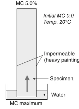
top and bottom faces were left uncoated. The bottom surface was submerged only a few millimeters in order to avoid buildup of hydrostatic pressure. The top surface was exposed to ambient conditions. The environmental labora-tory conditions were kept constant at 20°C and 40% relative humidity during the experiments (Fig. 2).
For all samples, moisture content (MC) was recorded at various time intervals. The moisture of each sample in grams was obtained by subtracting the moisture of the oven-dried samples from the moisture of the wet samples. After the absorption test, the specimen was cut consecu-tively into 24 to 27 pieces for measuring moisture and spe-cifi c gravity distributions. The volume for the spespe-cifi c gravity was measured by the water immersion method after both uncoated surfaces were coated with paraffi n.
Results and discussion
Maximum moisture content
The estimation of maximum MC is important in predicting the sorption process of wood accurately, which should be
defi ned at the boundary conditions. Most maximum MC values estimated by using Eq. 4 were slightly higher than the measured values; hemlock was the exception. This may be due to lower FSP, air entrapment, or dead pores. The difference in hardwood was higher than in softwood. However, Eq. 4 can be used to gauge an approximate value of maximum MC.
Estimation of moisture diffusivity
Moisture content changes with time, and moisture distribu-tions at the fi nal stage are shown in Fig. 3. The moisture diffusivity values in Tables 2 and 3 were obtained by the Boltzmann transformation method over the whole moisture content.12
However, the input values of b0 and b1 were
approximated using Eq. 9.
The shape of the curve representing the dependence of diffusion coeffi cients with moisture content was similar in all wood, and the diffusivity decreased with moisture content until the FSP was reached and then increased. Adapting them to the moisture transfer equation (Eq. 12), the simula-tion results gave poor predicsimula-tions for moisture content changes with time and moisture distributions. This is because the Boltzmann transformation method is valid for a semi-infi nite volume and a linear correlation between moisture fl ux and the square root of time.
Mathematically, inverse problems belong to the class of ill-posed problems. The solution does not satisfy the general requirements of existence, uniqueness, and stability under
small changes to the input data.13
The inverse solutions are known to be very sensitive to small changes in input data resulting from measurement and modeling errors. There-fore, to improve the numerical convergence, the initial input values of parameters obtained by the Boltzmann transformation method were used as a fi rst approximation for the Levenberg-Marquardt method. Equation 9 for the moisture diffusivity below the FSP was used initial input values for the discontinuous model.
MC 5.0%
Initial MC 0.0 Temp. 20°C
Impermeable (heavy painting)
Specimen
Water MC maximum
Fig. 2. Schematic diagram of the moisture absorption test.
MC, Moisture content
Table 2. Diffusivities with the continuous function by the inverse method, Eq. 20
Species Duration (months)
a0 a1 a2 a3 F
LMa Bb
Softwood
Hemlock 1 −22.35 3.571 −7.875 3.849 0.161 0.777
2 −22.37 1.880 −4.050 1.969 0.102 0.160
Radiata pine 1 −21.05 −5.596 8.226 −2.714 0.524 0.608 2 −21.52 −6.264 8.237 −2.276 0.575 3.001
Spruce 1 −21.80 −4.354 8.995 −3.552 0.266 0.377
2 −21.49 −6.456 8.889 −2.592 0.408 0.438 Hardwood
Painted maple 1 −16.35 −17.63 24.09 −8.392 0.140 15.53
2 −18.14 −14.84 28.25 −13.37 0.125 7.092
Japanese elm 1 −21.01 −4.527 7.630 0.381 0.146 0.146
2 −21.62 −0.857 −6.190 8.955 0.361 0.469
Horn beam 1 −21.52 −3.563 −1.538 9.700 0.046 0.246
2 −21.45 −6.995 20.57 −12.78 0.016 0.020
Nondimensional time Avera ge moi stu re co ntent (kg/ kg) 0.0 0.2 0.4 0.6 0.8 1.0
Distance from wetted surface (mm)
Moi stu re co nt ent (kg /kg) 0.0 0.5 1.0 1.5 2.0 2.5 Nondimensional time Average moi s tu
re content (kg/kg)
0.0 0.2 0.4 0.6 0.8 1.0
Distance from wetted surface (mm)
Moisture conten t (kg/kg) 0.0 0.5 1.0 1.5 2.0 2.5 Nondimensional time Average moistu re con ten t (kg/kg) 0.0 0.2 0.4 0.6 0.8 1.0
Distance from wetted surface (mm)
M o isture content (k g/kg ) 0.0 0.5 1.0 1.5 2.0 Nondimensional time A v era ge m o is tur e co nte nt (k g/ kg ) 0.0 0.2 0.4 0.6 0.8 1.0 1.2
Distance from wetted surface (mm)
M o ist u re c o nt en t (k g /k g) 0.0 0.2 0.4 0.6 0.8 1.0 1.2 1.4 Nondimensional time Av era g e mo istu re con ten t (kg /kg ) 0.0 0.1 0.2 0.3 0.4 0.5 0.6
Distance from wetted surface (mm)
Mois ture co nte n t (k g/kg ) 0.0 0.2 0.4 0.6 0.8 1.0 1.2 Nondimensional time
0.0 0.2 0.4 0.6 0.8 1.0 0.0 0.2 0.4 0.6 0.8 1.0
0.0 0.2 0.4 0.6 0.8 1.0 0.0 0.2 0.4 0.6 0.8 1.0
0.0 0.2 0.4 0.6 0.8 1.0 0.0 0.2 0.4 0.6 0.8 1.0
Ave rage m o ist u re c o ntent (k g/kg ) 0.0 0.1 0.2 0.3 0.4 0.5
Distance from wetted surface (mm)
0 50 100 150 200 0 50 100 150 200
0 50 100 150 200 0 50 100 150 200
0 50 100 150 200 0 50 100 150 200
Mois ture cont ent (kg/ kg) 0.0 0.2 0.4 0.6 0.8 1.0
(a)Hemlock (b)Radiata pine
(c)Spruce (d)Painted maple
(e) Japanese elm (f) Horn beam
Table 3. Diffusivities with two step functions by the inverse method, Eq. 21
Species Duration (months)
a0 a1 a2 a3 b0 b1 F
LM Ba
Softwood
Hemlock 1 −24.83 9.567 −11.99 4.706 17.95 14.87 0.042 0.320
2 −22.58 2.552 −5.179 2.407 19.95 10.35 0.056 10.22
Radiata pine 1 −20.32 −14.49 18.70 −5.887 18.64 12.66 0.272 2.055
2 −21.59 −2.453 1.298 0.610 19.65 3.574 0.333 4.873
Spruce 1 −23.76 4.817 −1.515 −0.014 17.68 9.609 0.118 0.192
2 −20.27 −11.93 14.85 −4.384 15.96 21.40 0.059 0.664
Hardwood
Painted maple 1 −19.55 −10.29 18.67 −7.152 17.72 9.629 0.114 1.475
2 −25.12 16.79 −19.86 10.34 18.87 3.010 0.078 8.431
Japanese elm 1 −24.09 17.41 −32.35 22.32 13.74 34.61 0.064 0.115
2 −23.18 14.72 −33.27 22.41 15.69 19.33 0.078 0.901
Horn beam 1 −29.98 44.12 −82.70 52.86 19.26 11.15 0.028 0.153
2 −22.93 2.491 3.353 −3.284 19.37 10.86 0.037 0.330
a Equation 9 below the fi ber saturation point and Boltzmann transformation method in nonhygroscopic range
Fig. 3a–f. Comparison of measured and predicted average moisture content change and moisture distribution using two steps of moisture diffusivity by the Levenberg-Marquardt inverse method. a Hemlock, b radiata pine, c spruce, d painted maple, e Japanese elm, f horn beam. Measured: fi lled circles, 1 month; open circles, 2 months. Predicted: solid line, 1 month;
Comparing Tables 2 and 3, the discontinuous diffusivity model (Eq. 21) gave better prediction of the development of the internal moisture distributions in wood during sorp-tion than the continuous model (Eq. 20). Using the discon-tinuous diffusivity of Table 3, the simulation results are represented by solid lines in Fig. 3.
This study shows that there is a distinctive hygroscopic zone in wood, although both experimental and model-based determination of phase-separated transport properties is still one of the most disputed issues in moisture transport analysis.14
For liquid water sorption simulation, moisture diffusivity should be separated into hygroscopic and nonhy-groscopic zones and two step functions of diffusivity should be used rather than an effective diffusivity to improve the simulation results.
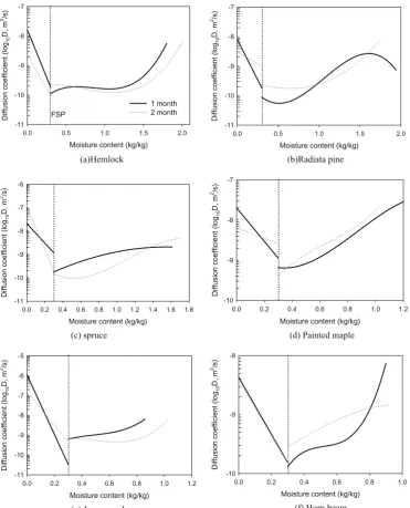
As shown in Fig. 4, the moisture diffusivity decreased with increasing moisture content until the FSP was reached
and it increased in the nonhygroscopic range, which agrees with other studies.7,11,15
For most species, the order of magnitude of moisture diffusivity is lies within the range of 10−8
to 10−10 m2
/s.
Conclusions
Using the Levenberg-Marquardt inverse technique, two diffusion models to predict moisture change with time and moisture distribution have been investigated for liquid water sorption. The moisture-dependent diffusivity was considered as a continuous function over the whole mois-ture range, while this coeffi cient was discontinuous at the fi ber saturation point. The initial input values of parameters by the Boltzmann transformation method were used to
Moisture content (kg/kg)
Diffusio
n coefficie
nt (lo
g10
D, m
2/s)
-11 -10 -9 -8 -7
1 month 2 month FSP
Moisture content (kg/kg)
Diffusi
on coefficie
nt (l
og
10
D,
m
2/s)
-11 -10 -9 -8 -7
Moisture content (kg/kg)
Dif
fusion coef
ficient
(log
10
D,
m
2/s)
-11 -10 -9 -8 -7 -6
Moisture content (kg/kg)
Di
ff
usi
on coe
ff
ici
ent
(l
og
10
D, m
2/s)
-10 -9 -8 -7
Moisture content (kg/kg)
Diffusion coefficient (log
10
D, m
2 /s)
-11 -10 -9 -8 -7 -6 -5
Moisture content (kg/kg)
Diffu
s
ion
coefficie
n
t
(log
10
D,
m
2/s
)
-10 -9 -8
0.0 0.5 1.0 1.5 2.0 0.0 0.5 1.0 1.5 2.0
(a)Hemlock (b)Radiata pine
0.0 0.2 0.4 0.6 0.8 1.0 1.2 1.4 1.6 1.8 0.0 0.2 0.4 0.6 0.8 1.0 1.2
(c) spruce (d) Painted maple
0.0 0.2 0.4 0.6 0.8 1.0 1.2 0.0 0.2 0.4 0.6 0.8 1.0
(e) Japanese elm (f) Horn beam
improve the numerical convergence as a fi rst approximation for the Levenberg-Marquardt method. Comparing the cal-culated moisture changes and profi les with experimental values, it is apparent that the discontinuous model using the parameters obtained by the inverse method is able to predict the development of the internal moisture distributions in wood during liquid water sorption. The results of this study should be useful in studying the process of sorption for exterior wood such as columns and dipping methods used for preservation treatments.
Acknowledgments This work was supported by the Korea Research Foundation Grant funded by the Korean Government (MOEHRD) (The Regional Research Universities Program/Biohousing Research Institute) and the Brain Korea 21 Program funded by the Ministry of Education, Republic of Korea.
References
1. Kang W, Chung WY, Eom CD, Yeo H (2008) Some considerations in heterogeneous nonisothermal transport models for wood: numerical study. J Wood Sci 54:267–277
2. Kang W, Kang CW, Chung WY, Eom CD, Yeo H (2008) The effect of openings on combined bound water and water vapor dif-fusion in wood. J Wood Sci 54:343–348
3. Koponen H (1987) Moisture diffusion coeffi cients of wood. Hemi-sphere, New York
4. Cloutier A, Fortin Y (1993) A model of moisture movement in wood based on water potential and the determination of the effec-tive water conductivity. Wood Sci Technol 27:95–114
5. Hukka A (1999) The effective diffusion coeffi cient and mass trans-fer coeffi cient of Nordic softwoods as calculated from direct drying experiments. Holzforschung 53:534–540
6. Rosen HN (1974) Penetration of water into hardwoods. Wood Fiber 5:275–287
7. Kumaran MK (1999) Moisture diffusivity of building materials from water absorption measurements. J Thermal Envel Build Sci 22:349–355
8. Mukhopadhyaya P, Kumaran K, Nordmandin N (2002) Effect of surface temperature on water absorption coeffi cient of building materials. J Thermal Envel Build Sci 26:179–195
9. Virta J, Koponen S, Absetz I (2006) Modelling moisture distribu-tion in wooden cladding board as result of short-term single-sided water soaking. Build Environ 41:1593–1599
10. Descamps F (1996) Continuum and discrete modeling of isother-mal water and air fl ow in porous media. PhD thesis, KU Leuven 11. Siau JF (1995) Wood: infl uence of moisture on physical properties.
Virginia Polytechnic Institute and State University, Blacksburg, VA
12. Kang W, Chung WY (2008) Estimation of moisture diffusivity during absorption by Boltzmann transformation method. Mokchae Konghak (in press)
13. Ozisik NM (1993) Heat conduction, 2nd edn. Wiley, New York 14. Couture F, Jomma W, Puiggali JR (1996) Relative permeability
relations: a key factor for a drying model. Transport Porous Media 23:303–335